Strong-coupling theory of counterions with hard cores between symmetrically charged walls

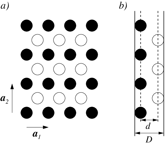
In the ground state, corresponding to infinite coupling ($\Xi\to\infty$), our interacting point charges in a slab domain stick to the domain’s boundary Earnshaw1842. In the case of symmetrically charged plates, $N/2$ particles stick on plate $\Sigma_{1}$ and the remaining $N/2$ particles stick on plate $\Sigma_{2}$. As $\eta$ goes from 0 to $\infty$, numerical simulations Falko94; Esfarjani95; Goldoni96; Schweigert99; Weis01; Messina03; Lobaskin07 indicate five distinct bilayer Wigner structures. For small and intermediate values of $\eta$ studied in this paper, the staggered rectangular structures I, II and III are relevant. As is shown in Fig. 1, a single layer consists in the rectangular lattice with the aspect ratio $\Delta$, defined by the primitive translation vectors $\bm{a}_{1}=a(1,0)$ and $\bm{a}_{2}=a(0,\Delta)$. The lattice spacing $a$ is determined by the electroneutrality requirement that the total surface charge in a rectangle must compensate the charge of just one particle, $a=\sqrt{q/(\sigma\Delta)}$. The identical rectangular structures on the two plates are shifted with respect to one another by a half period $(\bm{a}_{1}+\bm{a}_{2})/2$.

Structure I with $\Delta=\sqrt{3}$ corresponds to a (equilateral) triangular lattice which appears in the monolayer limit $\eta\to 0$. The aspect ratio is from the interval $1<\Delta<\sqrt{3}$ for soft structure II and $\Delta=1$ for structure III which is the staggered square bilayer. The phase transformation I–II takes place just at $\eta=0$ Messina03; Samaj12a, the phase transition between structures II and III appears at $\eta\sim 0.263$ and phase III provides the lowest energy up to $\eta\sim 0.621$.

Using techniques introduced in Ref. Samaj12a, the energy per particle $e_{0}=E_{0}/N$ is expressible for all three structures I-III in terms of the generalized Misra functions

$$z_{\nu}(x,y)=\int_{0}^{1/\pi}\frac{{\rm d}t}{t^{\nu}}{\rm e}^{-xt}{\rm e}^{-y/t};$$

(2.3)

the ordinary Misra functions correspond to $x=0$ Misra. In particular, writing

$$e_{0}(\eta,\Delta)\,=\,q^{3/2}\,\frac{e^{2}\sqrt{\sigma}}{\epsilon}\frac{1}{2\sqrt{\pi}}\Sigma(\eta,\Delta),$$

(2.4)

the function $\Sigma(\eta,\Delta)$ is expressed as an infinite series of the generalized Misra functions in Eq. (A4) of Appendix A. The generalized Misra functions $z_{\nu}(x,y)$ with half-integer indices can be written in terms of the complementary error function, see Eqs. (A2) and (A3) of Appendix A. This makes the use of symbolic calculation softwares very efficient. In practice, the infinite series (A4) over $(j,k)$ indices must be truncated at some $M$. For the well known case of the hexagonal lattice with $\eta=0$ and $\Delta=\sqrt{3}$, the truncation of the series at $M=1,2,3,4$ reproduces the Madelung constant up to $2,5,10,17$ decimal digits, respectively Samaj12a. To maintain a high accuracy of our results, we truncate all Misra series at $M=6$. The calculation of one ground-state energy value takes less than one second of CPU time on a standard PC.

For a given distance $\eta$, the value of the rectangular aspect ratio $\Delta$ is determined by the energy minimization condition

$$\frac{\partial}{\partial\Delta}e_{0}(\eta,\Delta)=0.$$

(2.5)

This condition sets the dependence of the aspect ratio on the dimensionless distance between the plates in the ground-state $\Delta_{0}(\eta)$, see Ref. Samaj12a.

The system being in thermal equilibrium at some (inverse) temperature $\beta=1/(k_{\rm B}T)$, there are two relevant length scales. The distance at which two elementary charges interact with thermal energy $k_{\rm B}T$ is the Bjerrum length

$$\ell_{\rm B}=\frac{\beta e^{2}}{\epsilon}.$$

(2.6)

A charge $qe$ at distance $z$ from a wall with the surface charge density $e\sigma$ has the potential energy $2\pi e^{2}q\sigma z/\epsilon$. The distance at which the charge $qe$ has the potential energy equal to thermal energy $k_{\rm B}T$ is known as the Gouy-Chapman length

$$\mu=\frac{1}{2\pi\ell_{\rm B}\sigma q}.$$

(2.7)

The coordinate $z$, which is perpendicular to the charged surfaces of the walls, will be often expressed in units of $\mu$, $\widetilde{z}=z/\mu$. The dimensionless coupling parameter $\Xi$, quantifying the strength of electrostatic correlations, is defined as the ratio of the two relevant lengths:

$$\Xi\,=\,\frac{q^{2}\ell_{\rm B}}{\mu}\,=\,2\pi\ell_{\rm B}^{2}\,\sigma\,q^{3}.$$

(2.8)

The strong-coupling (SC) regime $\Xi\gg 1$ is in practice most conveniently met by increasing the valence $q$. In doing so, excluded volume effects become prevalent, and the point-like limit of early studies less relevant. Alternatively, the regime of strong coupling corresponds to either low temperatures (a limit that is of little practical interest in view of applications with water, due to the unavoidable freezing of the solvent), or large surface charge densities. The lattice spacing $a$ of the Wigner structure, which is the characteristic length scale in the longitudinal $(x,y)$ plane, is much larger than $\mu$ in the SC regime as $a/\mu\propto\sqrt{\Xi}$. In the remainder, we take $q=1$, without loss of generality, in order not to clutter formulas.

For a single-layer Wigner crystal, experiments Grimes79 and simulations Morf79 give the estimate $\Xi\gtrsim 3\times 10^{4}$ for the coupling parameter at melting from the ordered crystal to a fluid phase. The coupling parameter at melting of the Wigner bilayer crystal depends on $\eta$ Goldoni96. Let $\Xi$ be large enough to localize particles near their Wigner-crystal positions. Within the canonical ensemble, the relevant thermodynamic quantities are the partition function $Z_{N}$ and the corresponding (dimensionless) free energy per particle $\beta f=\beta F/N$ which are defined, up to some irrelevant constants due to the interaction of surface charge densities with themselves and charged particles, as follows

$$Z_{N}=\frac{1}{N!}\int_{\Lambda}\prod_{i=1}^{N}\frac{{\rm d}^{3}r_{i}}{\lambda^{3}}\,{\rm e}^{-\beta E(\{{\bf r}_{i}\})},\quad\beta f=-\frac{1}{N}\ln Z_{N},$$

(2.9)

where $E(\{{\bf r}_{i}\})$ is the Coulomb interaction energy of the particles and $\lambda$ stands for the thermal de Broglie wavelength. We recall that the electric potential induced by the symmetrically charged plates is constant between the plates. The mean particle number density at point ${\bf r}$ is defined as $\rho({\bf r})=\left\langle\sum_{i=1}^{N}\delta({\bf r}-{\bf r}_{i})\right\rangle$, where $\langle\cdots\rangle$ means the statistical average over the canonical ensemble. It fulfils the conservation condition $\int\rho=N$ . We here study the $(x,y)$-averaged density profile $\rho(z)$, which depends only on the perpendicular $z$-coordinate, $\rho({\bf r})\equiv\rho(z)$, so that

$$\int_{0}^{d}{\rm d}z\,\rho(z)=\frac{N}{S}=2\sigma.$$

(2.10)

With the rescaled particle number density

$$\widetilde{\rho}(\widetilde{z})\equiv\frac{\rho(\mu\widetilde{z})}{2\pi\ell_{\rm B}\sigma^{2}},$$

(2.11)

the electro-neutrality condition (2.10) takes the form

$$\int_{0}^{\widetilde{d}}{\rm d}\widetilde{z}\,\widetilde{\rho}(\widetilde{z})=2.$$

(2.12)

The strong-coupling approach to the counterion system is based on a harmonic expansion of the energy $E$ with respect to particle coordinates around their ground state Wigner bilayer positions Goldoni96, where the ground state corresponds to infinite coupling. Numerical simulations in Ref. Samaj18 indicate that at finite although large coupling, the particles form another reference crystal of type I-III with the aspect-ratio parameter $\Delta$ which depends, besides the inter-plate distance $\eta$, also on the coupling constant $\Xi$, i.e. $\Delta(\Xi,\eta)$. We have performed the full harmonic expansion of particle coordinates around this reference crystal and fixed $\Delta(\Xi,\eta)$ of the reference crystal by minimizing the free energy with respect to this parameter. In this paper, we keep only the leading terms linear in $z$; it turns out that the harmonic deviations in the crystal $(x,y)$ plane as well as quadratic terms in the $z$-direction (proportional to $1/\sqrt{\Xi}$) have only minor effects on the results in the SC regime. The neglect of these terms will enable us to include the hard-core interactions in a relatively simple way. The total energy is thus expressed as

$$E(\{{\bf r}_{i}\})=Ne_{0}(\eta,\Delta)+\delta E,$$

(2.13)

where the energy change is given by

$$\beta\delta E=\kappa(\eta,\Delta)\left[\sum_{i\in\Sigma_{1}}\widetilde{z}_{i}+\sum_{i\in\Sigma_{2}}(\widetilde{d}-\widetilde{z}_{i})\right]+\cdots.$$

(2.14)

Here, the prefactor to small deviation terms is given by

	$\displaystyle\kappa(\eta,\Delta)$	$\displaystyle=$	$\displaystyle\frac{\eta}{2\pi}\sum_{i_{x},i_{y}}\frac{\Delta^{3/2}}{\left[\left(i_{x}-\frac{1}{2}\right)^{2}+\Delta^{2}\left(i_{y}-\frac{1}{2}\right)^{2}+\Delta\eta^{2}\right]^{3/2}}$		(2.15)
		$\displaystyle=$	$\displaystyle-\frac{1}{2\pi^{3/2}}\frac{\partial}{\partial\eta}\Sigma(\eta,\Delta)+1.$

The leading terms are linear in $\widetilde{z}_{i}$ for particles sitting in the ground state on plate $\Sigma_{1}$ and in $(\widetilde{d}-\widetilde{z}_{i})$ for particles $i\in\Sigma_{2}$. The function $\kappa$ can be viewed as an effective electric one-body field due to the uniform surface charges on the two plates and the particle ground-state layer on the opposite plate. For $\eta\to 0$ we have $\kappa\to 0$, i.e. each particle feels the zero field coming from the uniform surface charges on the plates while the effect of the opposite particle layer with the lattice spacing $a\gg d$ is negligible. For $\eta\to\infty$ we have $\kappa\to 1$, i.e. each particle feels the field coming from the surface charge at its own plate while the discrete counterion structure on the opposite plate is smeared out and neutralized by the opposite surface charge density on that plate. The function $\kappa$ thus reflects a continuous interpolation between the two-plate case for small $\eta$-values and the one-plate case for large $\eta$-values.

The partition function (2.9), with the particle interaction energy given by Eqs. (2.13) and (2.14), reads as

$$Z_{N}=\frac{1}{N!}\left(\frac{\mu}{\lambda}\right)^{N}\exp\left[-\beta Ne_{0}\right]Q_{z},$$

(2.16)

where

	$\displaystyle Q_{z}(\eta,\Delta)$	$\displaystyle=$	$\displaystyle\int_{0}^{\widetilde{d}}\prod_{i\in\Sigma_{1}}{\rm d}\widetilde{z}_{i}\,{\rm e}^{-\kappa\widetilde{z}_{i}}\int_{0}^{\widetilde{d}}\prod_{i\in\Sigma_{2}}{\rm d}\widetilde{z}_{i}\,{\rm e}^{-\kappa(\widetilde{d}-\widetilde{z}_{i})}$		(2.17)
		$\displaystyle=$	$\displaystyle\left(\frac{1-\exp(-\kappa\widetilde{d})}{\kappa}\right)^{N}.$

Neglecting irrelevant terms which do not depend on $\eta$ and $\Delta$, the leading SC representation of the free energy per particle is given by

$$\beta f(\eta,\Delta)=\frac{\sqrt{\Xi}}{2^{3/2}\pi}\Sigma(\eta,\Delta)-\ln\left(\frac{1-{\rm e}^{-\kappa(\eta,\Delta)\widetilde{d}}}{\kappa}\right).$$

(2.18)

The dependence of the aspect ratio $\Delta$ on the coupling constant $\Xi$ and the plate distance $\eta$, $\Delta(\Xi,\eta)$, is fixed by the principle of minimum free energy, i.e.,

$$\frac{\partial}{\partial\Delta}\beta f(\eta,\Delta)=0.$$

(2.19)

This condition is the analogue of the infinite coupling relation (2.5).

The pressure can be obtained via the thermodynamic route as follows

$$\beta P_{\rm th}=-\frac{\partial}{\partial d}\left(\frac{\beta F}{S}\right)=-2\sigma^{3/2}\frac{\partial(\beta f)}{\partial\eta}.$$

(2.20)

The pressure, rescaled as the particle density in (2.11), is given by

$$\widetilde{P}_{\rm th}\equiv\frac{\beta P_{\rm th}}{2\pi\ell_{\rm B}\sigma^{2}}=-\sqrt{\frac{2}{\pi\Xi}}\frac{\partial}{\partial\eta}\left[\beta f(\eta,\Delta)\right].$$

(2.21)

To assess the consistency of the result, it is appreciable to have an alternative route for computing the pressure. It is offered by the contact theorem contact, that requires the knowledge of the contact ionic density. The particle density profile is derived in appendix B. The contact theorem for planar walls relates the total contact density of particles on the wall and the pressure:

$$\widetilde{P}_{\rm c}=\widetilde{\rho}(0)-1=\kappa\left(\frac{1+{\rm e}^{-\kappa\widetilde{d}}}{1-{\rm e}^{-\kappa\widetilde{d}}}\right)-1.$$

(2.22)

The thermodynamic $\widetilde{P}_{\rm th}$ and contact $\widetilde{P}_{\rm c}$ pressures in general do not coincide in an approximate theory, although they refer to the same quantity. Their difference reveals the accuracy of the approach. It should be kept in mind that in (2.22), the local field $\kappa$ is distance dependent.

After having presented the key aspects of the theory for point ions, we now address hard-core effects: each ion is a hard-sphere of diameter $d_{\rm hc}$. The hard core is impenetrable to other particles (a model referred to as the primitive model) as well as the wall. We shall assume that the coupling constant $\Xi$ is very large, so that the Coulomb interactions dominate and a simple crystal phase (I, II, or III as in the point case with only one ion per lattice cell) is formed, as long as it does not lead to ionic overlap. Scanning only these simple crystal phases was further motivated by viscual inspection of the structures found by our Monte Carlo simulations. The counterions are supposed to be close to the Coulomb bilayer structure of type I-III, their centers being at distance $d_{\rm hc}/2$ from either of plates 1 or 2 and we shall look for steric hard-sphere effects on this structure.

If $D$ is the true distance between the walls, it is useful to define the reduced distance $d$ via $D=d+d_{\rm hc}$, where $d$ is the distance available to the center of mass of hard-sphere ions; it is equal to 0 in the extreme case when particles touch by their hard-core surfaces simultaneously both plates, see Fig. 1. As above, we use the notation $\eta=d\sqrt{\sigma}$. It is useful to express lengths in terms of the lattice spacing $a_{b}$ of the hexagonal Wigner bilayer at $\eta=0$ (with $\Delta=\sqrt{3}$), given by

$$\frac{\sqrt{3}}{2}a_{b}^{2}=\frac{1}{2\sigma}.$$

(3.1)

Structure I can exist at $\eta=0$ only if $d_{\rm hc}\leq a_{b}$. It is therefore natural to introduce the parameter

$$r\,\equiv\,\frac{d_{\rm hc}}{a_{b}}\,=\,d_{\rm hc}\sqrt{\sigma}\,3^{1/4}\,=\,\frac{3^{1/4}}{\sqrt{2\pi\Xi}}\widetilde{d}_{\rm hc}$$

(3.2)

which compares Coulomb and steric effects in the system. Note that $r=1$ when $d_{\rm hc}\sqrt{\sigma}=3^{-1/4}\simeq 0.76$. When $r<1$, the main expectation goes as follows. If $\Xi$ is sufficiently large, the ions strongly repel each other, so that their “in-plane” ($xy$) motion is essentially frozen: their only possible motion takes place perpendicularly to the plates, along $z$. It is consequently immaterial to consider point-ions, or hard-sphere ions, as long as $r<1$. We then expect that when expressed in terms of the $d$ variable, the pressure curves should be independent of the ionic diameter. This “no-hindrance regime” will be illustrated in section IV.

When $r>1$, steric hindrance impinges on the point-like arrangement, and needs to be properly addressed. Supposing that the counterions form basically the Coulomb bilayer structure of type I-III, there are strong steric hard-sphere restrictions on model parameters which have both intra-layer and inter-layer nature. We start by the intra-layer analysis. The existence of the structures I-III is limited by the condition $d_{\rm hc}\leq a(\Delta)=1/\sqrt{\sigma\Delta}$ which implies the restriction

$$\Delta\leq\frac{\sqrt{3}}{r^{2}}.$$

(3.3)

If $r\in[1,3^{1/4}]$, the formula (3.3) yields a restriction on the parameter $\Delta$. For $r>3^{1/4}\simeq 1.316$, the bilayer Wigner structures I-III cannot exist at all.

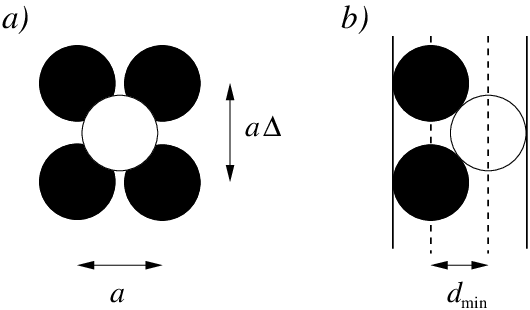
As concerns the inter-layer hard-core restrictions on structures I-III, there exists a minimal distance $d_{\min}$ at which the two layers can approach one another. This distance is determined as the one at which two nearest-neighbor hard-core particles from the opposite layers touch one another (see Fig. 2):

$$d_{\rm hc}^{2}=\left(\frac{\Delta a}{2}\right)^{2}+\left(\frac{a}{2}\right)^{2}+d_{\min}^{2}.$$

(3.4)

Equivalently,

$$\eta_{\min}^{2}(\Delta;r)=\frac{r^{2}}{\sqrt{3}}-\frac{1}{4}\left(\Delta+\frac{1}{\Delta}\right).$$

(3.5)

For a fixed $r$, the right-hand-side (rhs) of this equation is a monotonously decreasing function of $\Delta$ ($1<\Delta$). If $r\leq 3^{1/4}/\sqrt{2}=0.930605\ldots$, we have $\eta_{\min}=0$, i.e., there is no inter-layer restriction on structures I-III. For $r\geq 1$ it holds that $\eta_{\min}\geq 0$ for an arbitrary value of $\Delta\in[1,\sqrt{3}]$, i.e., there is always a hard-core restriction for distances between layers. For $r\in[0.930605,1]$, there is an interval of the aspect ratios $\Delta\in[1,\Delta^{*}(r)]$ with $\eta_{\min}\geq 0$ and an interval of $\Delta\in[\Delta^{*}(r),\sqrt{3}]$ with $\eta_{\min}=0$, $\Delta^{*}(r)$ being given by

$$\Delta^{*}(r)\,=\,\frac{2}{\sqrt{3}}r^{2}+\sqrt{\frac{4}{3}r^{4}-1}.$$

(3.6)

Figure 3 summarizes the situation, showing the domain of validity of the different regimes in the ($\Delta,r$) plane. Figure 4 shows how the minimum separation $\eta_{\min}$ and aspect ratio $\Delta$ are related, in the allowed domain. This domain is defined differently if $r<1$ and if $r>1$, see the caption, and also Fig. 5 which highlights the forbidden region for $r=0.99$. The reason for showing both data at $r=0.99$ and $r=1$ in Fig. 5 lies in the dashed curve, that shows how the geometry of the ground state problem without hard-core ($r=0$) depends on inter-plate distance $\eta$. This curve was obtained analytically in Samaj12a. It lies, although marginally, in the forbidden region of the $r=1$ case. Yet, it lies in the acceptable region with $r=0.99$. This allows to state that starting from the optimal ground state configuration of point charges, and gradually increasing the radius of hard sphere ions, steric effects will not alter the point-like configuration for $r<0.99$. They start to do so for $r$ slightly above 0.99.

For the limiting case $\eta_{\min}(\Delta,r)=0$, the two plates are allowed to touch one another ($d=0$). The equality $\eta_{\min}(\sqrt{3},r)=0$ is satisfied for $r=1$ which is the threshold beyond which $\eta_{\min}$ is positive. As soon as $\eta_{\min}>0$, the pressure is infinite for all inter-plate distances $\eta<\eta_{\min}$, since the hard spheres cannot be packed in such a small space.

The crystal state of the counterion system now depends not only on the coupling constant $\Xi$ but also on the $r$-parameter whose large value can decrease substantially the coupling constant $\Xi$ at which the crystal-fluid phase transition occurs. In the crystal phase, we can treat the hard-core system basically in the same way as the pointlike one in Sec. II, to obtain the effective (dimensionless) potential $-\kappa(\eta,\Delta)\widetilde{z}$ acting on particles at plate 1 and the symmetrically reflected one with respect to the slab center at $z=d/2$, $-\kappa(\eta,\Delta)(\widetilde{d}-\widetilde{z})$, acting on particles at plate 2. Because of strong Coulomb repulsions in the $(x,y)$ plane, particles move freely along the lines in the perpendicular $z$-direction defined basically by the ground-state structures I-III. Due to interlayer steric effects, the particles at plate 1 move in a reduced interval $\widetilde{z}\in[0,\widetilde{d}-\widetilde{d}_{\min}]$ while those at plate 2 in the interval $\widetilde{z}\in[\widetilde{d}_{\min},\widetilde{d}]$. In what follows, we shall use the following combination of variables:

$$h(\eta,\Delta;r)=\kappa(\eta,\Delta)\left[\widetilde{d}-\widetilde{d}_{\min}(\Delta;r)\right],$$

(3.7)

where $\widetilde{d}=\sqrt{2\pi\Xi}\,\eta$, with a similar relation between $\widetilde{d}_{\min}$ and $\eta_{\min}$.

Finally, previous works Samaj11; Samaj18 have shown that even when the ionic system is not coupled enough to be in its crystal phase but rather exhibits a strongly modulated liquid structure, the large-$\Xi$ calculations are nevertheless relevant as an approximate approach. The main reason is that both structures, liquid and solid, do exhibit the common feature of a correlation hole around each ion Moreira02; Palaia18. We thus here develop a theory that is grounded in the large-$\Xi$ regime, the relevance of which at moderate couplings has to be assessed by a direct comparison to numerical simulations.

To account for steric effects on the Coulomb free energy in the leading SC order (2.18), let us take one of the particles at plate $\Sigma_{2}$ as the reference ion. It has just four nearest neighbors at the corners of one rectangular plaquette of the Wigner crystal at plate $\Sigma_{1}$; we denote these particles by 1,2,3,4 and their perpendicular positions respectively by $\widetilde{z}_{1}$, $\widetilde{z}_{2}$, $\widetilde{z}_{3}$, $\widetilde{z}_{4}$. Because the particles are supposed to move along the lines determined by Wigner layers in the perpendicular $z$-direction, from among four positions only the maximal one $\max(\widetilde{z}_{1},\widetilde{z}_{2},\widetilde{z}_{3},\widetilde{z}_{4})$ is relevant. The original interval $[\widetilde{d}_{\min},\widetilde{d}]$ accessible to the reference particle is thus reduced to $[\widetilde{d}_{\min}+\max(\widetilde{z}_{1},\widetilde{z}_{2},\widetilde{z}_{3},\widetilde{z}_{4}),\widetilde{d}]$, see Fig. 6. The contribution of the reference particle on plate 2 to the partition function can be integrated out as follows

	$\displaystyle\int_{\widetilde{d}_{\min}+\max(\widetilde{z}_{1},\widetilde{z}_{2},\widetilde{z}_{3},\widetilde{z}_{4})}^{\widetilde{d}}{\rm d}\widetilde{z}\,{\rm e}^{-\kappa(\widetilde{d}-\widetilde{z})}\phantom{aaaaa}$
	$\displaystyle=\frac{1}{\kappa}\left[1-{\rm e}^{\kappa\max(\widetilde{z}_{1},\widetilde{z}_{2},\widetilde{z}_{3},\widetilde{z}_{4})-h}\right],$		(3.8)

where $h=\kappa(\widetilde{d}-\widetilde{d}_{\rm min})$, is a rescaled measure of available space. Performing the above procedure independently for every of $N/2$ particles on plate 2, the $N$-particle partition function reduces to the one of $N/2$ particles at plate 1,

	$\displaystyle Q_{z}$	$\displaystyle=$	$\displaystyle\frac{1}{\kappa^{N/2}}\int_{0}^{h}\prod_{i\in\Sigma_{1}}{\rm d}\widetilde{z}_{i}\,{\rm e}^{-\kappa\widetilde{z}_{i}}$		(3.9)
			$\displaystyle\times\prod_{{\rm plaq}(i)}\left[1-{\rm e}^{\kappa\max(\widetilde{z}_{i1},\widetilde{z}_{i2},\widetilde{z}_{i3},\widetilde{z}_{i4})-h}\right],$

where the product is over all $i=1,2,\ldots,N/2$ plaquettes of the Wigner rectangular lattice at plate 1, the coordinates of particles localized at the four corners of plaquette $i$ being denoted as $\widetilde{z}_{i1}$, $\widetilde{z}_{i2}$, $\widetilde{z}_{i3}$ and $\widetilde{z}_{i4}$. We see that the elimination of one half of particles implies plaquette four-particle interactions among the remaining half of particles. Finally, making the substitution $s_{i}=\kappa\widetilde{z}_{i}$ one ends up with

	$\displaystyle Q_{z}$	$\displaystyle=$	$\displaystyle\frac{1}{\kappa^{N}}\int_{0}^{h}\prod_{i=1}^{N/2}{\rm d}s_{i}\,{\rm e}^{-s_{i}}$		(3.10)
			$\displaystyle\times\prod_{{\rm plaq}(i)}\left[1-{\rm e}^{\max(s_{i1},s_{i2},s_{i3},s_{i4})-h}\right].$

Through the original variables $\{s_{i}\}$, the plaquettes are coupled, which makes the statistical mechanics problem at hand untractable. We shall treat the partition function $Q_{z}$ approximatively by using the Gibbs-Bogoliubov inequality Feynman98:

$$-\ln\left({\rm Tr}\,{\rm e}^{-H}\right)\leq{\rm Tr}\left(p_{0}\ln p_{0}\right)+{\rm Tr}\left(p_{0}H\right),$$

(3.11)

where $p_{0}$ is any normalized probability distribution, ${\rm Tr}\,p_{0}=1$. Comparing this formula with the studied case (3.10), we identify the (dimensionless) Hamiltonian

$$H\equiv\sum_{i=1}^{N/2}s_{i}-\sum_{{\rm plaq}(i)}\ln\left[1-{\rm e}^{\max(s_{i1},s_{i2},s_{i3},s_{i4})-h}\right]$$

(3.12)

and

$${\rm Tr}\equiv\int_{0}^{h}\prod_{i=1}^{N/2}{\rm d}s_{i}.$$

(3.13)

Let us choose

$$p_{0}(s_{1},s_{2},\ldots,s_{N/2})=\left(\frac{\alpha}{1-{\rm e}^{-\alpha h}}\right)^{N/2}\prod_{i=1}^{N/2}{\rm e}^{-\alpha s_{i}},$$

(3.14)

where $\alpha$ is a free (real) parameter. The reason for this choice is dictated by the observation of ionic density profiles, see below, that appear essentially exponential. In other words, $\alpha$ plays the role of a multiplying factor to the local effective electric field, dressed by steric effects. In absence of hard-core interactions, one would have precisely $\alpha=1$, and the treatment of section II would apply. The fact that $\alpha\neq 1$ (with an effective field $\alpha\kappa$) will be a direct signature of hard-core interactions. Our choice of trial probability $p_{0}$ decouples the plaquette, as mean-field treatments do. Since

$${\rm Tr}\left(p_{0}\ln p_{o}\right)=\frac{N}{2}\left[\ln\alpha-\ln\left(1-{\rm e}^{-\alpha h}\right)-\frac{1-(1+\alpha h){\rm e}^{-\alpha h}}{1-{\rm e}^{-\alpha h}}\right]$$

(3.15)

and

$${\rm Tr}\left(p_{0}H\right)=\frac{N}{2\alpha}\frac{1-(1+\alpha h){\rm e}^{-\alpha h}}{1-{\rm e}^{-\alpha h}}-2N\alpha\,\frac{\int_{0}^{h}{\rm d}s\,{\rm e}^{-\alpha s}\left(1-{\rm e}^{-\alpha s}\right)^{3}\ln\left(1-{\rm e}^{s-h}\right)}{\left(1-{\rm e}^{-\alpha h}\right)^{4}},$$

(3.16)

we obtain that

	$\displaystyle-\frac{1}{N}\ln Q_{z}$	$\displaystyle\leq$	$\displaystyle\ln\kappa+\frac{1}{2}\left[\ln\alpha-\ln\left(1-{\rm e}^{-\alpha h}\right)\right]+\frac{1}{2}\left(\frac{1}{\alpha}-1\right)\frac{1-(1+\alpha h){\rm e}^{-\alpha h}}{1-{\rm e}^{-\alpha h}}$		(3.17)
			$\displaystyle-2\alpha\,\frac{\int_{0}^{h}{\rm d}s\,{\rm e}^{-\alpha s}\left(1-{\rm e}^{-\alpha s}\right)^{3}\ln\left(1-{\rm e}^{s-h}\right)}{\left(1-{\rm e}^{-\alpha h}\right)^{4}}.$

Consequently, the free energy of hard spheres with the Coulomb interaction satisfies the inequality

	$\displaystyle\beta f(\eta,\Delta;r)$	$\displaystyle\leq$	$\displaystyle\frac{\sqrt{\Xi}}{2^{3/2}\pi}\Sigma(\eta,\Delta)+\ln\kappa(\eta,\Delta)+\frac{1}{2}\left[\ln\alpha-\ln\left(1-{\rm e}^{-\alpha h}\right)\right]+\frac{1}{2}\left(\frac{1}{\alpha}-1\right)\frac{1-(1+\alpha h){\rm e}^{-\alpha h}}{1-{\rm e}^{-\alpha h}}$		(3.18)
			$\displaystyle-2\alpha\,\frac{\int_{0}^{h}{\rm d}s\,{\rm e}^{-\alpha s}\left(1-{\rm e}^{-\alpha s}\right)^{3}\ln\left(1-{\rm e}^{s-h}\right)}{\left(1-{\rm e}^{-\alpha h}\right)^{4}}.$

The free parameter $\alpha$ is chosen to minimize the upper bound for the free energy, i.e., the rhs of this equation. In all the cases studied, the obtained $\alpha$ is in the interval $[1,\infty]$. The parameter $\alpha$ thus increases the slope of the decay of the particle density from the wall surface; since the density profile is normalized this automatically means the increase of the particle density at the wall as the consequence of the hard-core repulsion from particles close to the opposite wall. This can be thought of as a generalized depletion effect, where ions are pushed to their nominal plate by hard core, that adds to the Coulomb repulsion already at work for point particles. As before, the aspect ratio of the rectangular lattice $\Delta$ is also the minimizer of the free energy, respecting the hard-core restriction (3.3). The (rescaled) thermodynamic pressure is given by formula (2.21).

We turn to the density profile. Its part due to the particles in the vicinity of plate 1, $\rho_{1}(z)$, is obtained in analogy with the case of pointlike particles by introducing the generating Boltzmann factor $w({\bf r})$, see Appendix B. This means that the dimensionless Hamiltonian (3.12) has to be substituted in the original expression for the whole partition function as follows $H\to H-\sum_{i=1}^{N/2}\ln w({\bf r}_{i})$. Within the Gibbs-Bogoliubov formalism, $\ln w({\bf r}_{i})$ appears in the evaluation of ${\rm Tr}(p_{0}H)$ and therefore this is just the trial distribution (3.14) which determines the particle density

$$\widetilde{\rho}_{1}(\widetilde{z})=\frac{\alpha\kappa}{1-{\rm e}^{-\alpha\kappa(\widetilde{d}-\widetilde{d}_{\min})}}{\rm e}^{-\alpha\kappa\widetilde{z}}\theta(\widetilde{d}-\widetilde{d}_{\min}-\widetilde{z}),$$

(3.19)

where $\theta$ denotes the Heaviside step function. Given the factorized form taken in Eq. (3.14), this result does not come as a surprise. Although particles at plate 2 have been integrated out within our approach, their contribution to the density profile is determined by its reflection $\widetilde{z}\to\widetilde{d}-\widetilde{z}$ symmetry as follows

$$\widetilde{\rho}_{2}(\widetilde{z})=\frac{\alpha\kappa}{1-{\rm e}^{-\alpha\kappa(\widetilde{d}-\widetilde{d}_{\min})}}{\rm e}^{-\alpha\kappa(\widetilde{d}-\widetilde{z}}\theta(\widetilde{z}-\widetilde{d}_{\min}).$$

(3.20)

The total density of particles is given by

$$\widetilde{\rho}(\widetilde{z})=\widetilde{\rho}_{1}(\widetilde{z})+\widetilde{\rho}_{2}(\widetilde{z}).$$

(3.21)

In the analogous formula for pointlike particles (B5), the Coulombic effects are expressed through the function $\kappa\in[0,1]$ which is coupled to $\widetilde{z}$ and $\widetilde{d}-\widetilde{z}$ in exponentials. Now there is an additional multiplication parameter $\alpha\in[1,\infty]$ which reflects the “squeezing” effect of the ionic hard core.

The contact version of the pressure follows from the contact theorem (2.22). We have to distinguish between two cases. If $\widetilde{d}_{\min}\leq 0$, the particles from plate 2 can touch plate 1 and therefore

	$\displaystyle\widetilde{P}_{c}$	$\displaystyle=$	$\displaystyle\widetilde{\rho}_{1}(0)+\widetilde{\rho}_{2}(0)-1$		(3.22)
		$\displaystyle=$	$\displaystyle\alpha\kappa\left(\frac{1+{\rm e}^{-\alpha\kappa\widetilde{d}}}{1-{\rm e}^{-\alpha\kappa(\widetilde{d}-\widetilde{d}_{\min})}}\right)-1.$

If $\widetilde{d}_{\min}>0$, the particles from plate 2 cannot touch plate 1 and therefore

$$\widetilde{P}_{c}=\widetilde{\rho}_{1}(0)-1=\frac{\alpha\kappa}{1-{\rm e}^{-\alpha\kappa(\widetilde{d}-\widetilde{d}_{\min})}}-1.$$

(3.23)

To put to the test the analytic theory, we run Metropolis Monte Carlo simulations of the system composed of two symmetrically charged surfaces with counterions in-between, at various coupling parameters, separations and hard core radii. For each simulation, we use 512 spherical counterions, which all have their charge located in the center of their hard core. The planar surfaces are modeled as uniformly charged structureless hard walls. Long-ranged electrostatic interactions are handled by three-dimensional Ewald summation techniques with corrections for quasi-2-dimensionality, by adding vacuum slabs on each side of the charged walls (as described elsewhere A; B; Samaj18). We verified that our vacuum slabs were large enough in order not to influence our results (i.e., pressures and profiles), typically larger than a couple of thousands of Gouy–Chapman lengths defined in (2.7). Besides standard particle trial displacements, we also utilize floppy-box moves at constant box volume at which counterions are displaced conformally: either by shear or coupled biaxial compression-decompressions (where we compress one axis and decompress the other) both in the plane parallel to the surfaces. Trial move parameters were set such to have an acceptance ratio between roughly 20 and 50% for each case. Pressures and profiles at a fixed separation, a given counterion hard core radius, and a given coupling parameter are estimated by first equilibrating for $10^{4}$ Monte Carlo cycles and then sampling over $10^{5}$ subsequent cycles, where a cycle consists of either 512 trial counterion displacements or a trial floppy box move (a fifth of the total cycles). Pressures are evaluated both at the walls (contact theorem) or over the mid-plane by sampling the concentration (entropic contribution), ion-ion correlation (electrostatic energy), and hard-core repulsion (impulse) over the mid-plane Guldbrand84. Both measures give the same results within statistical errors. The mid-plane evaluation is usually less noisy and hence all simulation results are reported using this measure. We apply block averaging of ten blocks to estimate the precision in pressures. Starting configurations for our simulations are counterion bilayers of structure I if $r<1$ otherwise structure II with $\Delta$ equal to the upper bound of Eq. (3.3), compatible with the minimum separation.

Figure 7 shows the numerical results of the equation of state for six different coupling parameters. The two first and lowest ones, $\Xi=0.175$ and $\Xi=1.58$, yield similar pressure curves. Note that the point-like limit provides a universal equation of state, independent of $\Xi$ provided it is not too large (less than 2). This point-like limit is here in excellent agreement with Poisson-Boltzmann theory results (not shown). Beyond point ions, steric effects result in very similar pressure curves at the two lowest $\Xi$ studied; these effects are responsible for the relevance of the $a$ parameter (or equivalently $a_{b}$), for scaling out results. These two equations of states are repulsive, irrespective of the hard core radius and separation, with pressure curves increasingly repulsive when increasing hard core radii at a given separation. These low-$\Xi$ results serve as a reference to our strong-coupling analysis, illuminating the importance of increasing electrostatic coupling. Two peaks appear at these low coupling parameters, one at $\eta\simeq 0.4$ when $d_{\rm hc}\sqrt{\sigma}=0.7$ (cyan symbols) and the other at $\eta\simeq 1.5$ when $d_{\rm hc}\sqrt{\sigma}=1$. They are fingerprints of the pure hard core system, in this parameter range barely affected by the electric charges. For instance, the change of behaviour for $\eta\simeq 0.4$ and $d_{\rm hc}\sqrt{\sigma}=0.7$ is consistent with the confined hard-sphere phase diagram reported by Schmidt and Löwen Schmidt97. Indeed, computing the dimensionless quantities used in Schmidt97, we get $h\simeq 0.56$ and $\rho_{H}\simeq 0.64$, which corresponds to the onset of crystallisation, arriving from the fluid sector. Furthermore, for hard core radius $d_{\rm hc}\sqrt{\sigma}\lessapprox 0.4$ (or equivalently, $r\lessapprox 0.5$), only minor differences are seen compared to the $d_{\rm hc}=0$ situation in this low-coupling regime, where electrostatics can be described in a mean-field manner. We will see below when discussing the no-hindrance regime that this insensitivity is even more pronounced in the strong-coupling regime since it holds strictly for $r<1$, and also in a sense to be specified for $r>1$.

At $\Xi=17.5$, and at short separations, one observes a shallow attraction between the two surfaces if the counterions radius is not too large, $\widetilde{d}_{\rm hc}<5.25$ (or $d_{\rm hc}\sqrt{\sigma}<0.5$). Pressure curves start to be influenced by hard core radius as soon as $\widetilde{d}_{\rm hc}\gtrapprox 4$. Increasing counterions size makes pressure curves repulsive at all separations for $\widetilde{d}_{\rm hc}\approx 5.25$, but with local minima for $r<1$ ($\widetilde{d}_{\rm hc}<7.98$). The peak at $\eta\simeq 0.5$ seen previously for low couplings and $d_{\rm hc}\sqrt{\sigma}=0.7$ appears also for the lower $d_{\rm hc}\sqrt{\sigma}$ values (0.5 and 0.6) at $\Xi=158$ to gradually disappear again at even higher coupling parameters. $\Xi=17.5$ is special in the sense that pressures are close to zero around $\eta=0.5$ for the point charge case and hence is sensitive for perturbations (e.g. introducing excluded volume) around this state. The local minimum seen for $d_{\rm hc}\sqrt{\sigma}=1$ for the low coupling limit persists up to $\Xi=17.5$, but vanishes somewhere in the range $\Xi=[17.5,158]$. Even though the pressures are in practice zero for the high coupling cases at $\eta=1.5$ we still do not see any effect of the hard core radius (in contradiction to the $\Xi=17.5$ case and states around $\eta=0.5$). The relative influence of hard core vs electrostatic interactions is also decreasing with increasing coupling parameter. By increasing $\Xi$, one turns the $r<1$ cases from repulsive at all separations to attractive, except in a narrow range close to zero separation, of extension given by the Gouy-Chapman length. Somewhere around $\Xi=1750$, one also turns cases with $r>1$ from purely repulsive to having an attractive pressure minimum. For our highest coupling parameter ($\Xi=175000$), we see that the $r\geq 1$ follows the $d_{\rm hc}=0$ curve up to the closest separation for the corresponding $r$. This can be viewed as an extension to the sector $r>1$ of the no-hindrance effect alluded to in section III: it indicates that under such strong couplings, the dominant effect is electrostatics, equivalent to that of point-like ions, while steric effects only matter through the forbidden overlaps. When no overlaps are involved, the Coulombic interactions are largely dominant. The case $r=1$ does, however, have a smaller minimum in absolute value compared to the $d_{\rm hc}=0$ case even though the closest approaches are the same. This can theoretical be understood as some of the preferred bilayer structures are forbidden due to hard core overlaps (see Fig. 5), leading to a slightly altered and weaker (in terms of attraction) pressure curve. We come back to this in the next subsection.

We have argued in section III that for $d_{\rm hc}<a_{b}$, all pressure curves $P(d)$ should collapse onto their point-ion limit, provided the coupling parameter $\Xi$ be large enough. This no-hindrance regime is illustrated in Fig. 8. In this figure, the largest value of $r$ reported (respectively 0.92, 0.92 and 0.97 for panels a), b) and c)) is fairly close to 1. Yet, at the largest $\Xi$, this has no visible effect on the pressure curve, while the quality of the data collapse is altered when decreasing coupling $\Xi$. In the corresponding equation of state the increasing branch on the right hand side is actually universal, independent of coupling $\Xi$, when expressed in the proper variable, here $\eta$ Ivan; Palaia20, as revealed in Fig. 9. The reason behind this universality is that the behaviour is ruled by the infinite coupling attractor of point ions (with a divergent $\Xi$). The point-ion ground state pressure is indeed shown by the dashed line in Fig. 9. Besides, as hinted at in subsection IV.1, the no-hindrance effect extends to case with $r>1$, see Fig. 10. For $d_{\rm hc}>a_{b}$, i.e. $r>1$, it is seen that starting from large distances, the pressure curve follows the point counterion limiting curve, down to the smallest distance allowed by non overlap of hard cores. The minimal distance given by Eq. (3.5), matches very well that where $\widetilde{P}_{\rm tot}$ diverges in Fig. 10: for the data with $r\simeq 1.05$, we have $\eta_{\min}(\sqrt{3}/r^{2},r)\simeq 0.29$ (see also Fig. 4), while for $r\simeq 1.18$, we get $\eta_{\min}(\sqrt{3}/r^{2},r)\simeq 0.54$. Steric effects are here dichotomic: there are essentially irrelevant due to the strong Coulombic repulsion, or divergent at small $d$, for those configurations which are not allowed. Quite remarkably, the marginal situation with $r=1$ remains close to the point-ion attractor, down to vanishing distances where the two double layers on the opposite walls exactly register.

Before entering into a more precise comparison between analytical and numerical pressure profiles, we test the ansatz underlying our choice of trial exponential-type density $p_{0}$ in Eq. (3.14), by showing the ionic profiles in Fig. 11. The first observation is that they are neatly exponential in the vicinity of the plates, in line with our premises for the trial variational form for $p_{0}$. The profiles significantly deviate from their mean-field, Poisson-Boltzmann counterpart, shown with the dashed lines; on the scale of the figure, the different dashed lines corresponding to different separations are quasi-superimposed, but would depart at larger distances. We have predicted in section III that steric effects make the ionic profiles more peaked at the plates than the equivalent point-ion system, having the same available free space for center-of-mass displacement. This is corroborated by the MC data. This steric-driven enhanced localization is quantified, in the theory, by the parameter $\alpha$ appearing in (3.14) and (3.20). The predicted behaviour of $\alpha$ is shown in Fig. 12-left. When the plates are far away, $\alpha\to 1$, signalling that steric effect do not affect the local field $\kappa$, itself distance dependent, that maintains ions in the vicinity of a given plate. On the other hand, decreasing $\eta$, it is seen that $\alpha$ increases quite significantly. Besides, it is the product $\alpha\kappa$ that defines the local field; $\kappa$ decreases for decreasing $\eta$ while $\alpha$ shows the opposite trend, and we show in the inset of Fig. 12-left the resulting effects for the product, compared to the MC measures. These MC results are extracted from the slopes evidenced in Fig. 11. While the predicted trend seems correct, it is seen that the theory leads to too sharp of a dependence on the distance, while MC yields smoother curves. A similar comment applies to the aspect ratio parameter, displayed in Fig. 12-right. Our variational treatment captures the correct trend, but exaggerates the sharpness of the crossover. We note nevertheless that the agreement between MC and the prediction improves, expectedly, when increasing $\Xi$. It can be noted that the distance range where the predicted $\Delta$ underestimates the measured one is precisely where the localisation parameter $\alpha$ in Fig. 12-left displays a non-monotonous local bump. It is also worthwhile here to inspect directly structural features. Fig. 13 shows the projected instantaneous position of ions, which reveals that the arrangement is of type considered in the theoretical analysis, with rectangular unit cells. From left to right, the aspect ratio $\Delta$ decreases from 1.53 to a value close to 1, as also shown in Fig. 12-right. This is confirmed by the computation of the in-plane pair correlation function, as displayed in Fig. 14, which also illustrates the relevance of $\Xi$ to maintain in-plane order at large separation.

Figure 15 shows a comparison of the pressures obtained from the analytical theory and numerical Monte Carlo simulations at coupling parameters $\Xi=158$, 1750, 175 000 and for various hard core radii of the counterions. We focus here on the $r>1$ cases. For $\Xi=158$, the analytic theory seems to underestimate the repulsive pressure due to the hard core (or equivalent overestimate the electrostatic attraction). Similar trend is seen at $\Xi=1750$ even though the theory yields pressures closer to the numerical results. For $\Xi=175000$, we find a good agreement between numerical results and theory. At $d_{\rm hc}\sqrt{\sigma}=1$ ($\widetilde{d}_{hc}=1050$, i.e. $r=3^{1/4}$), the numerical Monte Carlo data does however exhibit a significant level of noise. Besides, we have proposed two routes to compute the pressures, a mechanical and a thermodynamical one. Within an exact treatment, both results should coincide. The fact that they yield relatively close results in Fig. 15 assesses the self-consistency of the approach proposed.

To summarize, the agreement between our analytical calculations and the Monte Carlo results is good at the highest coupling studied, where steric effects either do not alter the point-ion pressure, or forbid too close interplate distances, for which the pressure is infinite. Steric effects are thus here dichotomic, all or nothing. At smaller couplings, a crossover sets in, where hard core have a finite and non negligible contribution to the pressure, that we capture semi-quantitatively, see Fig. 15. Difference between the theory and simulation data are due to the mean-field nature of the variational prediction performed.

References

- (1) Y. Levin, Rep. Prog. Phys. 65, 1577 (2002).
- (2) D. Andelman, in Soft Condensed Matter Physics in Molecular and Cell Biology, edited by W.C.K. Poon and D Andelman (Taylor & Francis, New York, 2006).
- (3) T. Palberg, M. Medebach, N. Garbow, M. Evers, A. Barreira Fontecha, H. Reiber, and E. Bartsch, J. Phys.: Condens. Matter 16, S4039 (2004).
- (4) Ph. Attard, Adv. Chem. Phys. 92, 1 (1996).
- (5) J. P. Hansen and H. Löwen, Annu. Rev. Phys. Chem. 51, 209 (2000).
- (6) R. Messina, J. Phys.: Condens. Matter 21, 113102 (2009).
- (7) A. Khan, B. Jönsson, and H. Wennerström, J. Chem. Phys. 89, 5180 (1985).
- (8) R. Kjellander, S. Marčelja, and J. P. Quirk, J. Colloid Interface Sci. 126, 194 (1988).
- (9) V. A. Bloomfield, Biopolymers 31, 1471 (1991).
- (10) D. C. Rau and A. Pargesian, Biophys. J. 61, 246 (1992); ibid. 61, 260 (1992).
- (11) P. Kékicheff, S. Marčelja, T. J. Senden, and V. E. Shubin, J. Chem. Phys. 99, 6098 (1993).
- (12) K. Komorowski, A. Salditt, Y. Xu, H. Yavuz, M. Brennich, R. Jahnand and T. Salditt, Biophys. Journal 114 1908, (2018).
- (13) T. Mukhina, A. Hemmerle, V. Rondelli, Y. Gerelli, G. Fragneto, J. Daillant and T. Charitat, J. Phys. Chem. Lett. 10, 7195 (2019).
- (14) L. Fink, A. Steiner, O. Szekely, P. Szekely and U. Raviv, Langmuir 35, 9694 (2019).
- (15) K. Komorowski, J. Schaeper, M. Sztucki, L. Sharpnack, G. Brehm, S. Köster and T. Salditt, Soft Matter 16, 4142 (2020).
- (16) L. Guldbrand, B. Jönsson, H. Wennerström, and H. Linse, J. Chem. Phys. 80, 2221 (1984).
- (17) R. Kjellander and S. Marčelja, Chem. Phys. Lett. 112, 49 (1984).
- (18) D. Bratko, B. Jönsson, and H. Wennerström, Chem. Phys. Lett. 128, 449 (1986).
- (19) N. Grønbech-Jensen, R. J. Mashl, R. F. Bruinsma, and W. M. Gelbart, Phys. Rev. Lett. 78, 2477 (1997).
- (20) Although the dielectric constant of colloids in general differs from that of the surrounding medium (such as water) in which the counterions are immersed, one usually uses a simplified model with no such discontinuity and thus no dielectric images.
- (21) M. A. Gebbie, M. Valtiner, X. Banquy, E. T. Fox, W. A. Henderson, and J. N. Israelachvili, Proc. Natl. Acad. Sci. U. S. A. 110, 9674 (2013).
- (22) V. Valmacco , G. Trefalt , P. Maroni and M. Borkovec, Phys. Chem. Chem. Phys. 17, 16553 (2015).
- (23) C. Labbez, B. Jönsson, I. Pochard, A. Nonat, and Bernard Cabane, J. Phys. Chem. B 110, 9219 (2006).
- (24) A. M. Smith, A. A. Lee, and S. Perkin: J. Phys. Chem. Lett. 7, 2157 (2016).
- (25) Y. Jing, V. Jadhao, J. W. Zwanikken, and M. Olvera de la Cruz; J. Chem. Phys. 143, 194508 (2015).
- (26) S. F. Edwards and A. Lenard, J. Math. Phys. 3, 778 (1962).
- (27) Ph. Attard, D. J. Mitchell, and B. W. Ninham, J. Chem Phys. 88, 4987 (1988); 89, 4358 (1988); R. Podgornik, J. Phys. A 23, 275 (1990); R. R. Netz and H. Orland, Eur. Phys. J. E 1, 203 (2000).
- (28) A. G. Moreira and R. R. Netz: Europhys. Lett. 52, 705 (2000); Phys. Rev. Lett. 87, 078301 (2001).
- (29) R. R. Netz: Eur. Phys. J. E 5, 557 (2001).
- (30) A. G. Moreira and R. R. Netz: Eur. Phys. J. E 8, 33 (2002).
- (31) M. Kanduč and R. Podgornik, Eur. Phys. J. E 23, 265 (2007); Y. S. Jho, M. Kanduč, A. Naji, R. Podgornik, M. W. Kim, and P. A. Pincus, Phys. Rev. Lett. 101, 188101 (2008).
- (32) I. Rouzina and V. A. Bloomfield, J. Phys. Chem. 100, 9977 (1996).
- (33) B. I. Shklovskii, Phys. Rev. E 60, 5802 (1999); Phys. Rev. Lett. 82, 3268 (1999).
- (34) V. I. Perel and B. I. Shklovskii, Physica A 274, 446 (1999);
- (35) S. Earnshaw, Trans. Cambridge Philos. Soc. 7, 97 (1842).
- (36) V.I. Falko, Phys. Rev. B 49, 7774 (1994).
- (37) K. Esfarjani and Y. Kawazoe, J. Phys.: Condens. Matter 7 7217 (1995).
- (38) G. Goldoni and F. M. Peeters, Phys. Rev. B 53, 4591 (1996).
- (39) I. V. Schweigert, V. A. Schweigert, and F. M. Peeters, Phys. Rev. Lett. 82, 5293 (1999); Phys. Rev. B 60, 14 665 (1999).
- (40) J. J. Weis, D. Levesque, and S. Jorge, Phys. Rev. B 63, 045308 (2001).
- (41) R. Messina and H. Löwen, Phys. Rev. Lett. 91, 146101 (2003); E. C. Oǧuz, R. Messina, and H. Löwen, Europhys. Lett. 86, 28002 (2009).
- (42) V. Lobaskin and R. R. Netz, Europhys. Lett. 77, 38003 (2007).
- (43) L. Šamaj and E. Trizac, Europhys. Lett. 98, 36004 (2012); Phys. Rev. B 85, 205131 (2012).
- (44) R. D. Misra, Math. Proc. Cambridge Philos. Soc. 36, 173 (1940); M. Born and R. D. Misra, Math. Proc. Cambridge Philos. Soc. 36, 466 (1940).
- (45) L. Šamaj and E. Trizac, Phys. Rev. Lett. 106, 078301 (2011); Phys. Rev. E 84, 041401 (2011).
- (46) E. Trizac and L. Šamaj, in Proceedings of the International School of Physics Enrico Fermi, edited by C. Bechinger, F. Sciortino and P. Ziherl, Vol. 184 (2013), p. 61.
- (47) L. Šamaj, M. Trulsson, and E. Trizac, Soft Matter 14, 4040 (2018).
- (48) Y. G. Chen and J. D. Weeks, Proc. Natl. Acad. Sci. U. S. A. 103, 7560 (2006); J. M. Rodgers, C. Kaur, Y. G. Chen, and J. D. Weeks Phys. Rev. Lett. 97, 097801 (2006).
- (49) S. Nordholm, Chem. Phys. Lett. 105, 302 (1984).
- (50) C. D. Santangelo, Phys. Rev. E 73, 041512 (2006).
- (51) M. M. Hatlo and L. Lue, EPL 89, 25002 (2010).
- (52) A. Bakhshandeh, A. P. dos Santos, and Y. Levin, Phys. Rev. Lett. 107, 107801 (2011).
- (53) I. Palaia, M. Trulsson, L. Šamaj, and E. Trizac, Mol. Phys. 116, 3134 (2018).
- (54) H. N. Lekkerkerker and R. Tuinier, Colloids and the Depletion Interaction, Lecture Notes in Physics 833 (Springer, 2011).
- (55) M. Schmidt and H. Löwen, Phys. Rev. E 55, 7228 (1997).
- (56) I. Borukhov, D. Andelman, and H. Orland, Phys. Rev. Lett. 79, 435 (1997).
- (57) C. N. Patra and S. K. Ghosh, J. Chem. Phys.117, 8938 (2002).
- (58) M. S. Kilic, M.Z. Bazant, and A. Ajdari, Phys. Rev. E 75, 021502 (2007).
- (59) J. P. Valleau, R. Ivkov, and G. M. Torrie, J. Chem. Phys. 95, 520 (1991).
- (60) R. Kjellander, T. Akesson, B. Jönsson, and S. Marčelja, J. Chem. Phys. 97, 1424 (1992).
- (61) J. Zelko, A. Iglič, V. Kralj-Iglič, and P. B. S. Kumar, J. Chem. Phys. 133, 204901 (2010).
- (62) C. C. Grimes and G. Adams, Phys. Rev. Lett. 42, 795 (1979).
- (63) R. H. Morf, Phys. Rev. Lett. 43, 931 (1979).
- (64) D. Henderson and L. Blum, J. Chem. Phys. 69, 5441 (1978); D. Henderson, L. Blum, and J. L. Lebowitz, J. Electroanal. Chem. 102, 315 (1979); S. L. Carnie, D.Y.C. Chan, J. Chem. Phys. 74, 1293 (1981); H. Wennerström, B. Jönsson, and P. Linse, J. Chem. Phys. 76, 4665 (1982).
- (65) R. P. Feynman, Statistical Mechanics: A Set of Lectures (Westview Press, 1998).
- (66) I.-C. Yeh and M. L. Berkowitz, J. Chem. Phys. 111, 3155 (1999).
- (67) M. Mazars, J.-M. Caillol, J.-J. Weis and D. Levesque, Condens. Matter Phys. 4, 697 (2001).
- (68) I. Palaia, Charged systems in, out of, and driven to equilibrium: from nanocapacitors to cement, PhD, Paris-Saclay University (2019).
- (69) I. Palaia, A. Goyal, E. del Gado. L. Šamaj and E. Trizac, to be published.
- (70) In Fig. 1-a) indeed, the triangular lattice corresponds to having .
- (71) A. Schlaich, A.P. dos Santos, R.R. Netz, Langmuir 35, 551 (2019).
- (72) I. S. Gradshteyn and I. M. Ryzhik, Table of Integrals, Series, and Products, 6th ed. (Academic, London, 2000).
- (73) I. Travěnec and L. Šamaj, Phys. Rev. E 92, 022306 (2015).
- (74) F. Paillusson and E. Trizac, Phys. Rev. E 84, 011407 (2011).