Finding the Homology of Decision Boundaries with Active Learning

Let $\mathcal{X}$ be a Euclidean space that denotes the domain/feature space of our learning problem and let $\mu$ denote the standard Lebesgue measure on $\mathcal{X}$. We will consider the binary classification setting in this paper and let $\mathcal{Y}=\{0,1\}$ denote the label set. Let $p_{XY}$ denote a joint distribution on $\mathcal{X}\times\mathcal{Y}$. Of particular interest to us in this paper is the so-called Bayes decision boundary $\mathcal{M}=\{\mathbf{x}\in\mathcal{X}|p_{Y|X}(1|\mathbf{x})=p_{Y|X}(0|\mathbf{x})\}$. Indeed, identifying $\mathcal{M}$ is equivalent to being able to construct the provably optimal binary classifier called the Bayes optimal predictor:

Following along the lines of [5], the premise of this paper relies on supposing that the set $\mathcal{M}$ is in fact a reasonably well-behaved manifold¹¹ 1 Note that it is conceivable that the decision boundary is not strictly a manifold. While this assumption is critical to the rest of this paper, it is possible to extend the results here by following the theory in [12]. We will leave a thorough exploration of this for future work.. That is, we will make the following assumption.

The condition number $\frac{1}{\tau}$ is an intrinsic property of $\mathcal{M}$ (assumed to be a submanifold of $\mathbb{R}^{d}$) and encodes both the local and global curvature of the manifold. The value $\tau$ is the largest number such that the open normal bundle about $\mathcal{M}$ of radius $r$ is embedded in $\mathbb{R}^{N}$ for every $r<\tau$. E.g., in Figure 1, where $\mathcal{M}$ is a circle in $\mathbb{R}^{2}$ and $\tau$ is its radius. We refer the reader to the Appendix A (or [13]) for a formal definition.

Now we will suppose that we have access to $N$ i.i.d samples $\mathcal{D}=\{\mathbf{x}_{1},...,\mathbf{x}_{N}\}\subset\mathcal{X}$ that are drawn according to the marginal distribution $p_{X}$. Notice that in a typical passive learning setting, we assume access to $N$ i.i.d samples from the joint distribution $p_{XY}$. The goal of this paper is to demonstrate that we may obtain labels for far fewer labels than $N$ while achieving similar performance to the passive learning setting if we are allowed to sequentially and adaptively choose the labels observed. Based on the observed data, we define the set $\mathcal{D}^{0}=\{\mathbf{x}\in\mathcal{D}:f(\mathbf{x})=0\}$, that is the set of all samples with Bayes optimal label of 0; similarly, we let $\mathcal{D}^{1}=\{\mathbf{x}\in\mathcal{D}:f(\mathbf{x})=1\}$.

As outlined in Section 1, our goal is to recover the homological summaries of $\mathcal{M}$ from data. Homological summaries such as Betti numbers estimate the number of connected components and the number of holes of various dimensions that are present in $\mathcal{M}$. Since we only have a sample of data points in practice, we first construct a simplicial complex from these points that mimics the shape of $\mathcal{M}$. We can then estimate the rank of any homology group $H_{i}$ of dimension $i$ from this complex. This rank is called the Betti number $\beta_{i}$ and informally denotes the number of holes of dimension $i$ in the complex. The multi-scale estimation of Betti numbers, which involves gradual “thickening” of the complex, results in a persistence diagram PD_i that encodes the birth and death time of the $i-$dimensional holes in the complex. For more background we refer the reader to [14].

In [5], the authors consider the passive learning setting for estimating the homology of $\mathcal{M}$ and propose a simplicial approximation for the decision boundary called the Labeled Čech (L$\check{\text{C}}$) Complex. We now provide a definition of this complex, letting $B_{\epsilon}(\mathbf{x})$ denote a ball of radius $\epsilon$ around $\mathbf{x}$. We refer the reader to the Appendix B or [5] for the more details.

The set $S$ is used to construct the L$\check{\text{C}}$ complex witnessed by the reference set $\mathcal{D}^{1}$. This allows us to infer that each vertex of the simplices $\sigma$ are within distance $\gamma$ to some point in $\mathcal{D}^{1}$. The authors in [5] show that, under certain assumption on the manifold and the distribution, provided sufficiently many random samples (and their labels) drawn according $p_{XY}$, the set $U=\bigcup_{\mathbf{x}_{i}\in\sigma}B_{\epsilon}(\mathbf{x}_{i})$ forms a cover of $\mathcal{M}$ and deformation retracts to $\mathcal{M}$. Moreoever, the nerve of the covering is homotopy equivalent to $\mathcal{M}$. The assumptions under which the above result holds also turns out to be critical to achieve the results of this paper, and hence we will devote the rest of this section to elaborating on these.

Before stating our assumptions, we need a few more definitions. For the distribution $p_{XY}$, we will let

In other words, $\mathfrak{D}$ denotes the region of the feature space where both classes overlap, i.e., both class conditional distributions $p_{X\mid Y}(\cdot\mid 1)$ and $p_{X\mid Y}(\cdot\mid 0)$ have non-zero mass. For any $r>0$, we let ${\rm Tub}_{r}(\mathcal{M})$ denote a “tubular” neighborhood of radius $r$ around $\mathcal{M}$ [13]. Furthermore, we write ${\rm Tub}_{w}(\mathcal{M})$ to denote the smallest tubular neighborhood enclosing $\mathfrak{D}$. A stylized example that highlights the relationship between these parameters is shown in Figure 1. In the sequel, we will introduce the related assumption and the lemma underlying the results of this paper (similar to those in [13, 5]). All assumptions and follow-on results are dependent on two parameters that are specific to the joint distribution: $w$ - the amount of overlap between the distributions and $\tau$ - the global geometric property of the decision boundary manifold.

A principal difference between [13] and our work is that [13] has direct access to the manifold and supposes that all generated samples are contained within ${\rm Tub}_{(\sqrt{9}-\sqrt{8})\tau}(\mathcal{M})$; this is one of the sufficient conditions for manifold reconstruction from samples. In contrast, as in [5], we do not have direct access to the decision boundary manifold. Rather, certain properties of $\mathcal{M}$ are inferred from the labels. In this paper, we show that we can infer the homology of $\mathcal{M}$ with far fewer labels if we are allowed to sequentially and adaptively choose which labels to obtain.

Since the generated samples do not necessarily reside within ${\rm Tub}_{(\sqrt{9}-\sqrt{8})\tau}(\mathcal{M})$, it is not immediately apparent that it is possible to find an $S$ (see Definition 1) that is entirely contained in ${\rm Tub}_{(\sqrt{9}-\sqrt{8})\tau}(\mathcal{M})$. However, Assumption 2 allows us to guarantee precisely this. To see this, we will first state the following lemma.

That is, the lemma tells us that as long as we choose our sampling strategy to guarantee that both $\mathcal{D}^{0}$ and $\mathcal{D}^{1}$ are $\gamma/2$-dense in $\mathcal{M}$, and provided we choose $\gamma<(\sqrt{9}-\sqrt{8})\tau-w$, we can guarantee that $S\subset{\rm Tub}_{(\sqrt{9}-\sqrt{8})\tau}(\mathcal{M})$. $\mathcal{D}^{0}$ and $\mathcal{D}^{1}$ being $\frac{\gamma}{2}$-dense in $\mathcal{M}$ implies $\|\mathbf{x}_{i}-\mathbf{x}_{j}\|_{2}<\gamma$, where $\mathbf{x}_{i}\in\mathcal{D}^{0}\bigcap B_{\frac{\gamma}{2}}(\mathbf{p})$ and $\mathbf{x}_{j}\in\mathcal{D}^{1}\bigcap B_{\frac{\gamma}{2}}(\mathbf{p})$ for every $\mathbf{p}\in\mathcal{M}$.

Therefore, as the distance from $\mathbf{x}_{i}\in S\subseteq\mathcal{D}^{0}$ to $\mathbf{x}_{j}\in\mathcal{D}^{1}$ is bounded by $\gamma$ (see Definition 1(b)), $S$ is also $\frac{\gamma}{2}$-dense in $\mathcal{M}$. This immediately implies $S$ is $(w+\gamma)$-dense in $\mathcal{M}$. Therefore, with $S\subset{\rm Tub}_{(\sqrt{9}-\sqrt{8})\tau}(\mathcal{M})$, $S$ being $(w+\gamma)$-dense in $\mathcal{M}$ and an appropriate $\epsilon$ properly selected, we will have the $(\epsilon,\gamma)$-LČ complex homotopy equivalent to $\mathcal{M}$ per theorems in [5, 13]. We now state the following proposition.

A pictorial description of relations between $w$, $\gamma$ and $\tau$ is in Figure 1. In the stylized example in Figure 1, $\mathcal{M}$ is a circle, ${\rm Tub}_{w+\gamma}(\mathcal{M})$ is an annulus and the radius $\epsilon$ of the covering ball $B_{\epsilon}(\mathbf{x})$ is constrained by $\tau$.

A schematic diagram of the proposed active learning framework is presented in Figure 2. As illustrated, the framework starts from sampling sufficient unlabelled data from $p_{X}$. Subsequently, the framework takes as input an unlabeled dataset $\mathcal{D}$, and this dataset is used to generate an appropriate graph on the data. This graph is then used to iteratively query labels near the decision boundary. The subset of labeled samples are used to estimate the homology, resulting in the persistence diagram of the LČ complex. We briefly outline the label query and homology estimation phases below, and refer the reader to the appendices for the full details.

Let $G=(\mathcal{D},E)$ denote a $k$-radius neighbor graph constructed from the dataset $\mathcal{D}$. This allows us to define the cut-set $C=\{(\mathbf{x}_{i},\mathbf{x}_{j})|y_{i}\neq y_{j}\wedge(\mathbf{x}_{i},\mathbf{x}_{j})\in E\}$ and cut-boundary $\partial C=\{\mathbf{x}\in V:\exists e\in C\textrm{ with }\mathbf{x}\in e\}$. We begin by sketching a structural lemma about the graph $G$ and refer the reader to the Appendix D for a full statement and proof.

$\mathcal{D}^{0}$ and $\mathcal{D}^{1}$ being $\frac{\gamma}{2}$-dense in $\mathcal{M}$ indicates the longest distance between $\mathbf{x}_{i}\in\mathfrak{D}^{0}\bigcap B_{\frac{\gamma}{2}}(\mathbf{p})$ and $\mathbf{x}_{j}\in\mathfrak{D}^{0}\bigcap B_{\frac{\gamma}{2}}(\mathbf{p})$ for $\mathbf{p}\in\mathcal{M}$ is $\gamma$. Therefore, letting $k=\gamma$ as Lemma 2 suggested results in both $\mathcal{D}^{0}\bigcap\partial C$ and $\mathcal{D}^{1}\bigcap\partial C$ being $\frac{\gamma}{2}$-dense in $\mathcal{M}$. Similar to Lemma 2, constructing a graph with a $\gamma$ radius inevitably results in a subset of points in $\partial C$ leaking out of ${\rm Tub}_{w}(\mathcal{M})$ and we formally have $\partial C\subseteq{\rm Tub}_{w+\gamma}(\mathcal{M})$. The key intuition behind our approach is that $S^{2}$ is naturally turned to focusing the labels acquired within ${\rm Tub}_{w+\gamma}(\mathcal{M})$. As we show below, this is done in a remarkably query efficient manner, and furthermore, when we obtain labeled data via querying we can construct an LČ complex; this allows us to find the homology of the manifold $\mathcal{M}$. We next need some structural assumptions about the manifold $\mathcal{M}$.

Assumption 3(a) ensures sufficient mass in both classes such that $\mathcal{D}^{0}$ and $\mathcal{D}^{1}$ are $\frac{\gamma}{2}$-dense in $\mathcal{M}$. Assumption 3(b)(c) upper-bounds the measure of ${\rm Tub}_{w+\gamma}(\mathcal{M})$. Recall that $G=(\mathcal{D},E)$ in Lemma 2 is a labeled graph; we further write $\beta$ to denote the proportion of the smallest connected component with all the examples identically labeled. We lay out our main theorem as follows

We provide a complete proof of Theorem 1 in the Appendix D. However, we will provide some intuition about the operation of our algorithm, and hence to the proof of the theorem here.

The $S^{2}$ algorithm is split into two phases: uniform querying of labels and querying via path bisection. The uniform querying serves to finding a path connecting vertices of opposite labels. The path bisection phase queries at the mid-point of the shortest path that connects oppositely labeled vertices in the underlying graph. As the authors in [15] show, this endows $S^{2}$ with the ability to quickly narrow in on the cut-boundary $\partial C$. The uniform querying phase accounts for the first term in Eq. 2, which guarantees that there are sufficient paths to identify $\partial C$ completely. During the path bisection phase, we take $\left(\lceil\log_{2}|\mathcal{D}|\rceil+1\right)$ queries at most (this may be tightened using the techniques in [15]) to find the end point of the cut-edge inside a path; this needs to be done at most $|\partial C|$ to complete the querying phase. Next, with the Assumption 2 and the Lemma 2, it is guaranteed that $\partial C\subseteq{\rm Tub}_{w+\gamma}(\mathcal{M})\subset{\rm Tub}_{(\sqrt{9}-\sqrt{8})\tau}(\mathcal{M})$ with $\gamma$ properly selected following proposition 1. Therefore, we may use the measure $N_{w+\gamma}h_{w+\gamma}$ from Assumption 3(b)(c) to upper-bound $|\partial C|$ which results in the second term of Eq. 2. This naturally ties the query complexity to the manifold complexity via $N_{w+\gamma}$ and ${\rm Tub}_{w+\gamma}(\mathcal{M})$. Eq. 3 comes from the necessary condition for the LČ complex being homotopy equivalent to $\mathcal{M}$, following along the lines of [5].

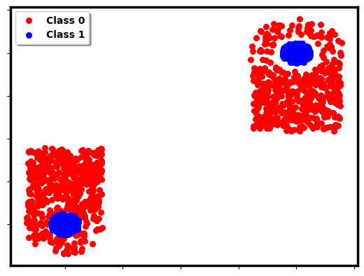
The synthetic data in Figure 3 has decision boundaries that are homeomorphic to two disjoint circles. This dataset has 2000 examples. Clearly from Figure 3, $\beta_{1}$ of the decision boundary is two.

Per the first step of our active learning algorithm, we construct a $k$-radius NN graph with $k=0.65$. The scale parameter is set assuming we have full knowledge of the decision boundary manifold. Subsequently, we use $S^{2}$ to query the labels of examples on the created graph. After the label query phase, we construct the LS-LVR complex with the queried samples and compute $\beta_{1}$ and PD₁ using the Ripser package  [16] and its interface [17]. For the passive learning baseline, we uniformly query the examples with all other aspects of the experiment remaining identical to the active case. We also compute $\beta_{1}$ and PD₁ from the complete dataset and consider them as the “ground-truth" homology summaries. We evaluate the similarities between the estimated homology summaries and the ground-truth homology summaries to show the effectiveness of our active learning framework.

We compare the bottleneck distance [18, 19] between the ground-truth and estimated values of PD₁ for different percent of data labeled. These results are shown on Figure 4. As is clear from the figure, the bottleneck distance for our active learning framework decreases faster than the passive learning approach and perfectly recovers the homology with only 50% of data. A visualization of the query process is shown on Figure 5. As expected, the active learning framework selects more examples to query near the decision. Please refer to the Appendix F to evaluate the performance of the active learning framework for different $k$-radius near neighbor graphs and $\beta_{1}$ recovery.

To demonstrate the effectiveness of our active learning framework on real data, we consider the classifier selection problem discussed in [5]. A bank of pretrained classifiers is accessible in the marketplace and customers select a proper one without changing the hyperparameters of the selected classifier. We consider two selection strategies as follow. One is topologically-based where the classifier with the smallest bottleneck distance from PD₁ of queried data is selected. The other one is to ensemble the topologically-selected classifier and the classifier selected based on the validation error of the queried data. We ensemble these two classifiers by averaging the output probabilities.

We split the data to a training set, a test set and an unlabeled data pool. The training set is used to generate four different banks of classifiers: $k$-NN with $k$ ranging from 1 to 29, SVM with polynomial kernel function degree ranging from 1 to 14, decision tree with maximum depth ranging from 1 to 27, and neural networks with the number of layers ranging from 1 to 6. The test set is used to evaluate the test error of each classifier. The unlabelled data pool is used to evaluate our active learning algorithm via selective querying.

We use the proposed active learning framework to estimate the homological properties of the queried data: constructing a $k$-nearest neighbors graph, query examples by $S^{2}$ and computing the PD₁ with the queried examples. We set $k=$3, 5, and 7. For passive learning, we keep all the operations the same as the active learning framework except the queried examples are collected by uniform random sampling. To compute the PD of the decision boundary of the classifier, we simply use the test set input and the classifier output. Having estimated the homological summaries from the queried data and the classifiers, we compute the bottleneck distance between the PD₁ of the queried data and the classifiers. For the non-ensemble method, we simply select the classifier having the smallest bottleneck distance as a topologically-selected classifier. For the ensemble method, we further include an additional classifier selected based on the validation error computed from the queried data and ensemble it with the topologically-selected classifier.

We implement the above procedure and evaluate on Banknote [20], MNIST [21] and CIFAR10 [22] datasets. Banknote contains 1372 instances in two classes with four input features for a binary classification task. We randomly sample 100 examples to construct the training set. Given the small size of the Banknote dataset, we use the remaining data as both the test set and unlabelled data pool. Although the test set and the data pool are not rigorously split in the Banknote case, it is still a fair comparison since the performance difference is only subject to the querying strategy. For the MNIST and the CIFAR10 datasets, we create (1) a 1 vs. 8 classification task from MNIST and (2) an automobile vs. ship classification task from CIFAR10. We randomly sample the data to create a training set with a sample size of 200, a test set with a sample size of 2000, and an unlabelled data pool with a sample size of 2000.

Table 3 shows the test error on banknote, MNIST and CIFAR10 for the classifier selected by querying 15% of the unlabelled data pool. We observe that the classifiers selected by our proposed active learning framework generally has a lower test error rate than the passive learning, especially in an ensemble classifier selection framework. As the experimental set-ups are identical (except for the querying strategy) we attribute the performance improvement to the proposed active learning framework used during model selection. Figure 6 indicates the performance of the non-ensemble classifiers selected by the homological similarities at the cost of the different proportions of the data pool. As expected, the proposed active learning framework achieves the best model selection faster than the passive learning for all classifier families. Note that the selection performance may be unstable with an increasing number of the queries since the active learning algorithm exhausts informative examples rapidly and begins to query noisy examples. In summary, Table 3 and Figure 6 indicate that the advantage of active learning in finding good homology summaries is also useful for model selection; this is evidenced by the lower error rates for the active learning approach relative to the passive learning approach.

We present the homological properties estimated by passive learning and the proposed active learning framework. Similar to the experiments with the synthetic dataset, we access the complete unlabelled data pool and their labels to compute $\beta_{1}$ and PD₁ and use them as the ground-truth $\beta_{1}$ and PD₁. On the other hand, we query the unlabelled data pool and estimate $\beta_{1}$ and PD₁ from the queried data. As we observe in the Figure 7(a), $\beta_{1}$ estimated by our active learning algorithm has a more similar trend to the ground-truth $\beta_{1}$ in all three real datasets. Furthermore, CIFAR10 has a significantly higher $\beta_{1}$ than MNIST and Banknote datasets indicating more complex decision boundaries. This is consistent with the Table 3 which shows that the error rates for the CIFAR10 binary classification tasks is higher than the other two datasets. Figure 7(b) shows the bottleneck distance between the estimated PD₁ and the ground-truth PD₁ for different proportions of labelled data. We observe that the active learning algorithm maintains a smaller bottleneck distance at early stages of querying. Such benefits gradually diminish as more of the data is labelled.

References

- [1] J. Schmidhuber, “Evolutionary principles in self-referential learning, or on learning how to learn: the meta-meta-… hook,” Ph.D. dissertation, Technische Universität München, 1987.
- [2] L. Morán-Fernández, V. Bolón-Canedo, and A. Alonso-Betanzos, “Can classification performance be predicted by complexity measures? a study using microarray data,” Knowledge and Information Systems, vol. 51, no. 3, pp. 1067–1090, 2017.
- [3] G. Kusano, Y. Hiraoka, and K. Fukumizu, “Persistence weighted gaussian kernel for topological data analysis,” in International Conference on Machine Learning, 2016, pp. 2004–2013.
- [4] C. Chen, X. Ni, Q. Bai, and Y. Wang, “A topological regularizer for classifiers via persistent homology,” arXiv preprint arXiv:1806.10714, 2018.
- [5] K. N. Ramamurthy, K. Varshney, and K. Mody, “Topological data analysis of decision boundaries with application to model selection,” vol. 97, pp. 5351–5360, 09–15 Jun 2019. [Online]. Available: http://proceedings.mlr.press/v97/ramamurthy19a.html
- [6] B. Rieck, C. Bock, and K. Borgwardt, “A persistent weisfeiler-lehman procedure for graph classification,” in International Conference on Machine Learning, 2019, pp. 5448–5458.
- [7] W. H. Guss and R. Salakhutdinov, “On characterizing the capacity of neural networks using algebraic topology,” arXiv preprint arXiv:1802.04443, 2018.
- [8] B. Rieck, M. Togninalli, C. Bock, M. Moor, M. Horn, T. Gumbsch, and K. Borgwardt, “Neural persistence: A complexity measure for deep neural networks using algebraic topology,” arXiv preprint arXiv:1812.09764, 2018.
- [9] K. R. Varshney and K. N. Ramamurthy, “Persistent topology of decision boundaries,” in 2015 IEEE International Conference on Acoustics, Speech and Signal Processing (ICASSP). IEEE, 2015, pp. 3931–3935.
- [10] T. K. Ho, M. Basu, and M. H. C. Law, “Measures of geometrical complexity in classification problems,” in Data complexity in pattern recognition. Springer, 2006, pp. 1–23.
- [11] C. Hofer, R. Kwitt, M. Niethammer, and A. Uhl, “Deep learning with topological signatures,” in Advances in Neural Information Processing Systems, 2017, pp. 1634–1644.
- [12] J. Kim, J. Shin, F. Chazal, A. Rinaldo, and L. Wasserman, “Homotopy reconstruction via the cech complex and the vietoris-rips complex,” in The 36th International Symposium on Computational Geometry (SoCG 2020), 2020.
- [13] P. Niyogi, S. Smale, and S. Weinberger, “Finding the homology of submanifolds with high confidence from random samples,” Discrete & Computational Geometry, vol. 39, no. 1-3, pp. 419–441, 2008.
- [14] H. Edelsbrunner and J. Harer, “Persistent homology - a survey,” Contemporary mathematics, vol. 453, pp. 257–282, 2008.
- [15] G. Dasarathy, R. Nowak, and X. Zhu, “S2: An efficient graph based active learning algorithm with application to nonparametric classification,” in Conference on Learning Theory, 2015, pp. 503–522.
- [16] U. Bauer, “Ripser: efficient computation of vietoris-rips persistence barcodes,” Aug. 2019, preprint.
- [17] N. Saul and C. Tralie, “Scikit-tda: Topological data analysis for python,” 2019. [Online]. Available: https://doi.org/10.5281/zenodo.2533369
- [18] A. Efrat, A. Itai, and M. J. Katz, “Geometry helps in bottleneck matching and related problems,” Algorithmica, vol. 31, no. 1, pp. 1–28, 2001.
- [19] M. Kerber, D. Morozov, and A. Nigmetov, “Geometry helps to compare persistence diagrams,” Journal of Experimental Algorithmics (JEA), vol. 22, pp. 1–20, 2017.
- [20] D. Dua and C. Graff, “UCI machine learning repository,” 2017. [Online]. Available: http://archive.ics.uci.edu/ml
- [21] Y. LeCun, L. Bottou, Y. Bengio, and P. Haffner, “Gradient-based learning applied to document recognition,” Proceedings of the IEEE, vol. 86, no. 11, pp. 2278–2324, 1998.
- [22] A. Krizhevsky, G. Hinton et al., “Learning multiple layers of features from tiny images,” 2009.
- [23] H. A. Edwards and A. J. Storkey, “Towards a neural statistician,” ArXiv, vol. abs/1606.02185, 2016.
- [24] A. Bridgwater, “Enough Training, Let’s Get Down To The AI Supermarket,” Forbes, Sep 2018. [Online]. Available: https://www.forbes.com/sites/adrianbridgwater/2018/09/18/enough-training-lets-get-down-to-the-ai-supermarket/#5f13cdbc10c3
- [25] R. W. Ghrist, Elementary applied topology. Createspace Seattle, 2014, vol. 1.