KCWI observations of the extended nebulae in Mrk 273

We observed Mrk 273 with KCWI on the Keck II telescope on June 14 and 15, 2018. We used the blue low-dispersion (BL) grating and medium slicer with KCWI, which provides a spectral resolution of $R=1800$, a spaxel size of $0.29\times 0.69^{\prime\prime}$, and a FOV of $20^{\prime\prime}\times 16^{\prime\prime}$ per pointing. We configured the articulating camera to a central wavelength of $4500\AA$ and used a detector binning of $2\times 2$, yielding wavelength coverage of $3435–5525\AA$. The seeing was $0.8^{\prime\prime}$, corresponding to a projected distance of 0.62 kpc at the redshift of our target. Since the angular size of Mrk 273 exceeds the FOV of the IFU, we defined six pointing areas to cover the galaxy. The footprint of our KCWI pointings are shown in Figure 1, overlaid on the HST/ACS [OIII] image in 51. Each pointing area was observed for 30 to 60 minutes, consisting of individual exposures of 10 minutes for the nuclear region, and 15 minutes for the extended regions. Individual exposures in each pointing area were dithered $0.35^{\prime\prime}$ along slices to subsample the output spaxels. For the nuclear region, we took a 1-minute exposure for each dither position to sample pixels saturated in the 10-minute exposure.

We reduced the data using the KCWI Data Extraction and Reduction Pipeline v1.1.0 and the IFSRED library (Rupke 2014a). We first performed a correction to saturated pixels in raw frames of the nuclear region using the routine IFSR_KCWISATCOR. This routine searches for saturated pixels in the 10-minute exposure of the nuclear region, and replaces them with pixels in its corresponding 1-minute exposure after scaling for the exposure time difference. The corrected frames of the nuclear pointing region and raw frames of other pointing regions are then passed to the pipeline. The default wavelength calibration produced large residuals of $\approx 1\AA$, resulting from a mismatch with the pipeline thorium-argon (ThAr) atlas, so we selected DISPLAY mode 3 to manually accept and reject lines matched by the pipeline. The residuals of the resulting wavelength solutions were reduced to $\approx 0.3\AA$. Sky subtraction was performed using the pipeline with manual selection of a sky mask region in each frame. For pointings in the nuclear region, where the source occupies the entire FOV, we used a sky frame from a nearby pointing that was observed immediately before or after the nuclear pointing. Following the full pipeline stages, we resampled the data onto $0.29^{\prime\prime}\times 0.29^{\prime\prime}$ spaxel grids using the routine IFSR_KCWIRESAMPLE, and generated a mosaic of the data using the routine IFSR_MOSAIC. The resulting stacked data cube has dimensions of $166\times 215$ spaxels, covering $48.1^{\prime\prime}\times 62.4^{\prime\prime}$ and corresponding to projected physical dimensions of $37.1~\mathrm{kpc}\times 48.1~\mathrm{kpc}$ at $z=0.0373$.

KCWI has a remarkable capability to map low surface brightness extended emission. The left panel of Figure 3 shows the mosaic image of the stellar continuum emission at $3600-5000\AA$ (wavelengths near emission lines have been masked). A prominent feature is the well-known tidal tail (e.g. Kim et al. 2002; 51; 64) extending to the south of the galaxy, which is common in galaxies in the late stage of a merger event²² 2 See Figure 5 of Cox et al. 2008 for the simulation of a merger between a galaxy pair with a stellar ratio of 10:1 at 3.6–4 Gyr with a strikingly similar morphology.. This image covers $\sim 12$ kpc of the tidal tail; the full extent is up to $\sim 36$ kpc (Kim et al. 2002, e.g). We also observe weak diffuse continuum emission in the northeast of the galaxy reported in 51.

The middle panel of Figure 3 shows the continuum-subtracted [OIII]4959+5007 mosaic image. The emission image was constructed by integrating $\pm 675$ $\mathrm{km~s}^{-1}$around the doublet and subtracting nearby continuum on both sides.³³ 3 For clarity, we note that the emission line maps presented in this Section are different from the initial line maps used to generate Voronoi bins. The brightest [OIII] emission is in the central 10 kpc of the galaxy, which we call the nuclear region in this paper. In the Figure, we mark the locations of the two known AGNs, the nuclear superbubble in 57 and the “outflow regions” in 51. The nuclear superbubble extends in the N-S directions about the nuclei, with the northern half coinciding with a relatively bright region in [OIII], and the southern half with a relatively faint region in [OIII]. This is consistent with the effect of extinction and the superbubble being a bipolar outflow, with blueshifted gas in the north and redshifted gas in the south (see Section III.3 for details). The “outflow regions” defined by 51 lie ENE and WSW from the nucleus, corresponding to two bright regions in [OIII]. We note that these outflows regions are constructed in 51 to enclose regions of enhanced [OIII] emission immediately outside the nucleus, and their locations should not necessarily be taken as the direction of an outflow; we discuss this point further in Section IV.1.

We also detect in [OIII] the two previously-reported extended  nebulae (Armus et al. 1990; 51; 64). Extending from the ENE “outflow region”, a bright nebula of ionized gas is seen spanning at least 20 kpc from the nucleus in the northeast of the galaxy. This NE nebula contains several bright filamentary structures around its edge, and is hollow at the center, resembling an evacuated bubble or a loop. While it is in the general direction of the diffuse continuum emission, the line and stellar emission regions in this direction do not completely overlap, particularly in the northern part of the nebula. Another extended nebula is detected in [OIII] for the first time towards the southwest of the galaxy, west of the tidal tail. This SW nebula extends $\sim 20$ kpc from the nucleus. It is less luminous in [OIII] compared with the NE nebula. It approximately follows the direction of the tidal tail, but they are offset by $\sim 1-3$ kpc. A composite continuum and [OIII] image is shown in the right panel of Figure 3 for comparison.

Our wide-field IFU data allows us to map the flux and spatial distribution of numerous emission lines apart from the [OIII] doublet detected with KCWI. A key result of this paper is the detection and spatial mapping of the faint, high-ionization emission lines [NeV]3426, [OIII]4363 and [HeII]4686, which are useful as shock and AGN diagnostics. In addition, we map the emission from the low-ionization [OII]3726,9 doublet. Figure 4 shows the continuum-subtracted mosaic images of these emisison lines, integrating $\pm 675$ $\mathrm{km~s}^{-1}$ around the respective line centers at $z=0.0373$. The high-ionization [NeV]3426, [OIII]4363 and HeII4686 lines show the strongest emission in the nuclear region. Remarkably, these high-ionization lines are all observed to have extended emission in the NE nebula, in regions tracing the emission of the [OIII] doublet, but they are not detected in the SW nebula. On the other hand, the morphology of the low-ionization [OII] doublet emission is similar to that of the [OIII] doublet, but it is enhanced in the SW nebula.

Quantitative measurements of emission line fluxes are obtained using the emission-line fitting procedures on the Voronoi-binned data cube described in Section II.3.2. The left panel of Figure 5 shows the resulting Voronoi-binned model flux map of [OIII]5007, and the velocity profiles of three representative Voronoi bins from the nuclear region, NE nebula, and SW nebula. The nuclear bin has the broadest velocity profile, followed by the SW bin, while the NE bin has the narrowest profile. The detailed kinematic properties of the ionized gas are discussed below in Section III.3. In the right panel of Figure 5 we show the emission line spectra and best-fit multi-component models for the [NeV]3426, [OII]3726,9, H$\gamma$, [OIII]4363, HeII4686, $\mathrm{H}\beta$, and [OIII]5007 emission lines. The [OII] doublet, Balmer lines, and [OIII]5007 emission lines are detected in all three spatial bins shown in the left panel, while the higher-ionization [NeV]3426, [OIII]4363 and HeII4686 are only detected in the nuclear and NE bins, and not in the SW bin. The above properties are generally true for most Voronoi bins in each region. Three kinematic components are typically required in the nuclear region, one to two in the SW nebula, and one in the NE nebula.

In the SW region, a series of broad bumps accompanied by large flux variances are observed in the spectra near the bluest end of the wavelength coverage of our observation, possibly due to imperfect calibration or differential observing conditions during the exposures in this pointing. The [NeV]3426 emission line, which is within the wavelengths affected, is not detected in the SW bin. Two other high-ionization lines, [OIII]4363 and HeII4686, have lower ionization potentials than [NeV]3426 and are thus potentially more prominent. However, they are also undetected in the SW bin, even though they are not within the affected wavelengths. This forms a consistent picture that high-ionization lines are absent in the SW region. Therefore, the non-detection of the [NeV]3426 emission line in the SW bin is likely due to an intrinsic absence of the line rather than the large flux variance observed in that region.

Figure 6 presents a more complete spatial view of each emission line by showing the model flux maps of the [OII]3726,9 doublet, and the [NeIII]3869, $\mathrm{H}\beta$, [NeV]3426, [OIII]4363 and HeII4686 emission lines, using the emission line fits above. The [OII]3726,9 doublet, and the [NeIII]3869 and $\mathrm{H}\beta$ emission lines are generally detected in the nuclear, NE and SW regions. However, the high-ionization [NeV]3426, [OIII]4363 and HeII4686 emission lines are detected in only the nuclear and NE regions, and not in the SW region.

With the integral field KCWI data, we are able to map out the kinematics of the ionized gas in the galaxy and identify distinct kinematic structures within the system. An important result of this paper is the kinematics of the large scale ionized gas, i.e. the NE and SW nebulae. The velocity percentiles presented below are with respect to the total line profile resulting from the sum of all significant components. The upper left panel of Figure 7 shows the central velocity $v_{50}$, which is the 50th percentile of the velocity profile, traced by [OIII]5007. The systemic velocity is set to be the median of the central velocity of the stellar continuum. The nuclear region has a complex kinematic structure, with a redshifted region towards the southeast and north of the nucleus, and a blueshifted region towards the west and northeast. The large-scale SW nebula is generally blueshifted by $\sim 200-300$ $\mathrm{km~s}^{-1}$. The NE nebula has a mild redshift of $\sim 30-100$ $\mathrm{km~s}^{-1}$ in the eastern part of the nebula (seen as the left half in the figure), and is mildly blueshifted by $\sim 40-100$ $\mathrm{km~s}^{-1}$ in the western part (seen as the right half in the figure).

The upper right panel of Figure 7 shows the velocity dispersion $\sigma$ of [OIII]5007 across the galaxy. In the nuclear region, very broad emission with $\sigma>250$ $\mathrm{km~s}^{-1}$ is observed along the direction of the bipolar superbubbles in 57 (marked here as open black circles outlined with a solid line), but extends to $\sim 5$ kpc, approximately two to three times the previously-reported size of the superbubbles. The regions with the highest velocity dispersion ($\gtrsim 600\mathrm{km~s}^{-1}$) lie beyond the known extent of the superbubbles in the north and east directions. This suggests that the high-velocity outflowing gas in the superbubbles is substantially more extended that previously measured. Moderately broad emission with $\sigma\sim 150-250$ $\mathrm{km~s}^{-1}$ is observed in the “outflow regions” defined in 51, which extend $\sim 5$ kpc in both directions perpendicular to the superbubbles (marked here with open circles with dashed outlines). The larger scale extended nebulae have fairly uniform velocity dispersion, with the SW nebula showing $\sigma\sim 100-150$ $\mathrm{km~s}^{-1}$and the NE nebula showing a smaller dispersion of $\sigma\sim 50$ $\mathrm{km~s}^{-1}$.

The lower left and lower right panels of Figure 7 show the “maximum” redshifted and blueshifted velocities $v_{02}$ and $v_{98}$, which are the velocity that encompasses $2\%$ and $98\%$ of the cumulative velocity distribution, respectively. The southern superbubble contains highly redshifted emission with $v_{02}$ between 800 and 1400 $\mathrm{km~s}^{-1}$, while the northern superbubble contains highly blueshifted emission with $v_{98}$ bewteen $-1800$ and $-800$ $\mathrm{km~s}^{-1}$, consistent with a bipolar superbubble of fast moving outflows. Additionally, fast moving, redshifted gas with $v_{02}\gtrsim 900$ $\mathrm{km~s}^{-1}$ extends beyond the known superbubble towards a wedge-shaped region in the south up to $\sim 5$ kpc. Similarly, there is a wedge-shaped region of high-velocity blueshifted gas extending north up to $\sim 4$ kpc. This, combined with the velocity dispersion map, suggests that fast moving gas from the superbubbles extends two to three times beyond the previously-known extent. On larger scales, the NE nebula has “maximum” velocities up to $-200$ and 200 $\mathrm{km~s}^{-1}$, while the SW nebula generally has velocities between $-50$ and $500$ $\mathrm{km~s}^{-1}$.

The kinematics of the stellar emission is measured by fitting the continuum Voronoi-binned data cube described in Section II.3.1. The left panel of Figure 8 shows the resulting model flux map of the continuum, while the middle panel shows the central velocity of the stellar continuum $v_{*}$. On large scales, apart from the tidal tail, weak continuum in the NE is also detected. The stellar continuum near the nucleus is redshifted in the north-south direction, and blueshifted in the east-west direction. In addition, the weak continuum in the NE is generally blueshifted by $\sim 100$ $\mathrm{km~s}^{-1}$. To quantify how much the kinematics of the ionized gas decouples from the continuum, we calculate the central velocity of [OIII]5007 relative to that of the stellar continuum by subtracting spaxel-by-spaxel the $v_{*}$ map of the continuum from the $v_{50}$ map of [OIII]5007. We show the resulting map of $v_{50}-v_{*}$ in the the right panel of Figure 8. The ionized gas north of the nucleus is generally blueshifted relative to the stellar continuum, and generally redshifted in the south, despite the complex kinematic structure in [OIII]5007 alone. In addition, the NE nebula is generally redshifted from the stellar continuum by $\sim 50-100$ $\mathrm{km~s}^{-1}$, instead of displaying the two distinct redshifted and blueshifted halves as seen in [OIII]5007 alone.

An important goal of this paper is to investigate the origin of the ionized gas that produces the observed emission. From the numerous emission line maps presented for Mrk 273, one can obtain line ratio maps, which are crucial in diagnosing the physical conditions of the ionized gas in different regions of the galaxy. To obtain accurate line ratios, we first account for extinction across the galaxy. We calculated the reddening $E(B-V)$ in each Voronoi bin from the Balmer decrement of the total $\mathrm{H}\beta$ and H$\gamma$ emission line fluxes. We assumed Case B recombination at $10^{4}$ K and the Cardelli et al. 1989 extinction curve and $R_{V}=3.1$. The resulting reddening map is shown in Figure 9. Relatively strong reddening of $E(B-V)\gtrsim 0.5$ is observed in the the SW nebula as well as the inner nuclear region, while the NE nebula has weaker reddening of $\sim 0.2$. The median reddening of the galaxy is 0.19.

We constructed maps of line ratios commonly used as diagnostics before and after extinction correction, and show them in Figure 10. To correct for extinction, line fluxes in each Voronoi bin are calculated using the reddening map. For Voronoi bins without significant detection of the Balmer lines, the median reddening value across the galaxy is used to calculate the corrected flux. Extinction corrections lead to a median change in the line ratios of [OIII]5007/$\mathrm{H}\beta$, [OII]3726,9/[OIII]5007, HeII/$\mathrm{H}\beta$, and [OIII]4363/[OIII]5007 of -0.01, 0.09, 0.01, and 0.05 dex, respectively. We note that the change in the numerical values of the line ratios are modest, and the spatial trends seen in the line ratio maps are unchanged by extinction correction. Numerical values of line ratios in the rest of this subsection refer to the extinction-corrected values.

The NE nebula has high $\log(\mathrm{[OIII]5007}/\mathrm{H}\beta)$ line ratios of $\sim 1$ to 1.2, while these line line ratios are substantially lower in the SW nebula, with values of $\sim 0.2$ to 0.6. The $\log(\mathrm{[OIII]5007}/\mathrm{H}\beta)$ line ratios in the nuclear region have a complex structure. An interesting feature is that regions of high $\log(\mathrm{[OIII]5007}/\mathrm{H}\beta)$ line ratios extend in the northeast and southwest directions, coinciding with the “outflow region” (dotted circles), while regions of low line ratios extend in the north and south directions, aligning with the axis of the supperbubbles (circles with solid outlines).

The distribution of the $\log(\mathrm{[OII]3726,9/[OIII]5007})$ line ratio generally displays opposite trends to that of $\log(\mathrm{[OIII]5007}/\mathrm{H}\beta)$. While this is not entirely unexpected because of the inverse dependence on [OIII]5007 of the two line ratios, the different dynamic range of the line ratios indicates that this is also driven by differences in [OII]3726,9. $\log(\mathrm{[OII]3726,9/[OIII]5007})$ is the highest in the SW nebula, at $\sim 0.5$ to 1, and the lowest in the NE nebula, at $\sim-0.7$ to $-0.3$. In the nuclear region, the $\log(\mathrm{[OII]3726,9/[OIII]5007})$ line ratios are elevated along the direction of the superbubbles, and are lower in the “outflow regions”.

The $\log(\mathrm{HeII4686}/\mathrm{H}\beta)$ line ratio exhibits similar trends to $\log(\mathrm{[OIII]5007}/\mathrm{H}\beta)$. The NE nebula and the “outflow region” display enhanced line ratios, while the superbubbles have lower line ratios. For $\log(\mathrm{[OIII]4363/[OIII]5007})$, higher line ratios are observed along the superbubbles, and lower line ratios are observed in the “outflow region” and the NE nebula.

In this subsection, we use line ratio diagnostic diagrams to investigate the nature of the ionizing sources of the gas in different regions of Mrk 273. Figures 11 to 14 show the observed line ratios and predictions of ionization models on diagnostic diagrams. Line ratios are chosen to be either close in wavelength so that extinction effects are minimized, e.g. HeII4686/$\mathrm{H}\beta$ and [OIII]5007/$\mathrm{H}\beta$, or from the same species so that effects of an unknown metallicity are minimized, e.g. [OII]3726,9/[OIII]5007, [OIII]4363/[OIII5007] and [NeV]3426/[NeIII]3869 (Baldwin et al. 1981). In each diagnostic diagram, we denote line ratios of spaxels in the nuclear region, the NE nebula, and the SW nebula with different colors to analyze the ionization mechanism in each region. When an emission line is undetected in a region, we show in the diagnostic diagrams the median value of the $3\sigma$ upper limit in the spaxels of that region. For line ratios in the nuclear region, we further separate the spaxels in the slow, medium, and fast regions according to their velocity dispersion ($\sigma<200~\mathrm{km~s}^{-1}$, $200~\mathrm{km~s}^{-1}<\sigma<400~\mathrm{km~s}^{-1}$ and $\sigma>400~\mathrm{km~s}^{-1}$), and denote them with different colors. In the following, we use the IDL Tool for Emission-line Ratio Analysis (Groves & Allen 2010, ITERA; ) to explore models of different ionization mechanisms and compare them with the observed line ratios.

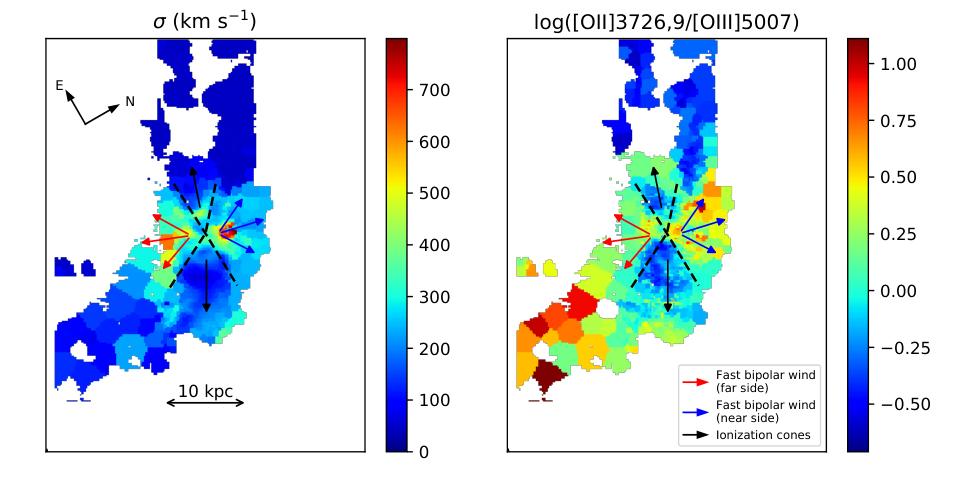
An important result of this study is the mapping of the kinematics of the ionized gas outflows in the nuclear region of Mrk 273. Along the N-S direction of the superbubble reported by 57, we detect high velocity gas with velocity dispersion $>250~\mathrm{km~s}^{-1}$ in two wedge-shaped regions extending in both directions, demarcated by black dashed lines in Figure 16. Moreover, the measurement of $v_{02}$ and $v_{98}$ shows the same wedge-shaped distribution of gas kinematics, with the N side blueshifted and the S side redshifted to maximum velocities up to $1800~\mathrm{km~s}^{-1}$. The wedges span about 5 kpc in radius and $\sim 90\arcdeg$ in opening angle, and are approximately $2-3$ times more extended than the reported radius of the superbubble and up to a factor of 10 larger in projected area. This clearly demonstrates a fast, extended, wide-angle, bipolar wind in the N-S direction, which was previously identified as a more localized superbubble. This illustrates the need of large FOV IFU observations in order to measure the true geometry and extent of outflows.

The fitting of the superbubble by 57 showed that the outflow center lies between the two AGNs, $0.4^{\prime\prime}$ from the N and $0.7^{\prime\prime}$ from the SW, while the uncertainty in the outflow center is $0.3^{\prime\prime}$. Around the N AGN, a rotating gas disk has been observed with its rotational axis oriented in the NNW-SSE direction, with a PA of $0\arcdeg$ to $-30\arcdeg$ (Downes & Solomon 1998; U et al. 2013; Aladro et al. 2018, e.g). This is consistent with the N-S collimation of the bipolar outflow if it is driven by the N AGN. On the other hand, a morphological stellar disk has been observed around the SW AGN by imaging, although it is not resolved for kinematic analysis (U et al. 2013; Medling et al. 2014). The SW disk is elongated along N-S direction, suggesting a rotational axis in the E-W direction. If it is indeed a rotating disk around the SW AGN, its orientation is not consistent with the N-S collimation of the bipolar outflow. Therefore, the most likely origin of the N-S bipolar outflow is the N AGN.

Another intriguing structure in Mrk 273 reported in the literature is the “outflow regions” defined in 51 in the ENE and WSW directions. These regions were selected from the regions with the brightest [OIII] detected in imaging data, and were measured to have disturbed kinematics in selected apertures in long-slit spectroscopy. As a result, the properties and origin of these “outflow regions”, such as whether they are a separate outflow from the N-S wind, were not clearly determined. The kinematic maps of the ionized gas show two wedge-shaped regions of lower velocity dispersion in approximately the E-W directions and between the N-S winds (demarcated by black dashed lines in Figure 16). The velocity dispersion of the E-W wedges is the highest closer to the nucleus and decreases with increasing radius. The “outflow regions” are situated at the inner tip of the wedges close to the nucleus, and have elevated velocity dispersion of $150-250~\mathrm{km~s}^{-1}$, compared with the median velocity dispersion of $143~\mathrm{km~s}^{-1}$ across the galaxy.

While emission line ratio diagnostics reveal contributions from shock plus precursor mixed with AGN photoionization in the entire nuclear region, there is a stronger contribution from AGN photoionization in the slower spaxels, corresponding to the E-W wedges in which the “outflow regions” are located. In fact, the line ratio maps also display the same wedge shaped structures in the E-W and N-S directions. We replicate the [OII]3726,9/[OIII]5007 line ratio map in Figure 16 and demarcate the wedges with black dashed lines. Considering the fact that the “outflow regions” are also the brightest regions in [OIII], combined with the stronger AGN photoionization contribution, the E-W wedges likely represent the ionization cones of one of the AGNs in the nucleus. As discussed above, the rotating disk around the N AGN has an axis in the N-S direction, while that around the the SW is in the E-W direction. Therefore, the E-W wedges most likely represent the ionization cones of the SW AGN.

The kinematics of the E-W wedges are more ambiguous. While the E-W wedges have an elevated velocity dispersion of $150-250~\mathrm{km~s}^{-1}$, the gas is not as fast as the N-S bipolar outflow, suggesting it is not the same phenomenon as the N-S outflow. On the other hand, the central velocity $v_{50}$ displays bipolar kinematics, with the E wedge redshifted to $\sim 100-200~\mathrm{km~s}^{-1}$ and the W wedge blueshifted to $\sim 100~\mathrm{km~s}^{-1}$. Measurements of $v_{02}$ and $v_{98}$ show maximum redshifted velocity of $500-600~\mathrm{km~s}^{-1}$ in the E wedge and maximum blueshifted velocity of $300-500~\mathrm{km~s}^{-1}$ in the W wedge, respectively. The bipolar kinematics are also observed in the central velocity relative to the stellar velocity ($v_{50}-v_{*}$, Figure 8), where the central velocity of the E-W wedges are shifted from the stellar continuum by $\sim 100$ $\mathrm{km~s}^{-1}$. The motion of the gas is decoupled from that of the stars, so the bipolar kinematics is not purely caused by rotation.

It is possible that the E-W wedges represent a slower gas outflow originating from the SW nucleus travelling along the direction of the ionization cone, as outflows are known to escape from paths of least resistance (Faucher-Giguère & Quataert 2012, e.g.). The well-defined collimation of the ionization cones, most clearly demonstrated in the line ratio maps (Figure 16), also suggests that they are fairly perpendicular to the line of sight, which can potentially explain the more modest velocity of the gas in the E-W wedges. The kinematics could also be produced by the remnants of a past outflow episode from the SW nucleus that has partially dissipated away its velocity.

One of the most striking features in the KCWI data is the extended NE nebula detected in multiple emission lines spanning over $20$ kpc in extent. The NE nebula displays a hollow morphology, which resembles a evacuated bubble possibly originating from a past outflow event (Rupke et al. 2019, e.g.). A particularly remarkable result from the line ratio diagnostics presented here is that the slow spaxels in the compact, nuclear region and the spaxels in the extended NE nebula reside in a very similar line ratio space in all of the diagnostic diagrams. Another clear correlation is that not only do both sets of spaxels have similar kinematics ($\sigma<200\mathrm{km~s}^{-1}$), they are also located in the same projected physical direction from the nuclei. The slow spaxels in the nuclear region are primarily located in the E-W wedges $\sim 1-5$ kpc ENE and WSW of the nucleus. The NE nebula is located $\sim 5-15$ kpc ahead of the E wedge, northeast of the nucleus. The similar line ratios, kinematics, and physical direction suggest a common source of ionization for the E-W wedges and the extended NE nebula.

One possible origin of the NE nebula suggested in the literature is tidal debris photoionized by an AGN (Rodríguez Zaurín et al. 2014; Spence et al. 2016). This is potentially supported by the diffuse stellar continuum emission at a similar location NE of the galaxy, which is due to tidal interactions. Moreover, the quiescent kinematics of the NE nebula is not indicative of an active outflow, which is typically kinematically broadened by turbulence to velocity dispersions of $\gtrsim 200\mathrm{km~s}^{-1}$. As the NE nebula is located along the ionization cone of the SW AGN, in this scenario, it can be tidally disrupted gas photoionized by the SW AGN. The shock contribution shown by line ratio diagnostics could potentially arise from the collision between gas clouds during tidal interactions.

Another possible origin of the NE nebula is one related to an outflow event. This is suggested by the bubble-like morphology of the nebula, which could be due to gas evacuated by an outflow (Rupke et al. 2019, e.g.). The kinematics of the NE nebula is relatively narrow (FWHM $\sim 120~\mathrm{km~s}^{-1}$), with a velocity shift with respect to the stellar continuum of $\sim 100~\mathrm{km~s}^{-1}$. While the kinematics are not suggestive of an active outflow, the nebula could result from a past outflow event, in which the gas has slowed down and dissipated away part of its turbulence. Such a scenario is possible given the complex outflow-related kinematics revealed by the KCWI data in the inner 5 kpc. While the fast bipolar wind is travelling in the N-S direction, and thus unlikely related to the NE nebula, the E side of the E-W wedges is in the same projected direction as the NE nebula. As the E-W wedges potentially represent the remnants of a past outflow episode originating from the SW nucleus that has dissipated part of its velocity (see Section IV.1 for discussion), and the NE nebula could be an extension of the remnants of the same outflow episode. Assuming an outflow velocity of $500~\mathrm{km~s}^{-1}$, the outflowing gas can reach 20 kpc in $\sim 40$ Myr. The shock contribution seen in the NE nebula could be produced when the outflow interacts with the ambient materials and dissipates away its velocity. Recent theoretical studies have noted that “cold” ($\sim 10^{4}$ K) outflowing gas extending large distances (e.g. $\sim 20$ kpc) can be produced as a result of a cycle of mixing between the hot and cold gas in a starburst-driven outflow and cooling (Armillotta et al. 2016; Gritton et al. 2017; Gronke & Oh 2018; Schneider et al. 2020, e.g.). Such scenarios can potentially provide a mechanism to explain the presence of $10^{4}$ K gas in the NE nebula at 20 kpc from the galactic center through an outflow episode. Alternatively, recent simulations have shown that such cold gas can arise if cosmic rays are the primary sources of momentum input to cold clouds (Brüggen & Scannapieco 2020).

The presence of the high-ionization [NeV]3426 emission line in a galaxy spectrum is commonly used as an indicator of AGN activity in galaxy surveys (Gilli et al. 2010; Mignoli et al. 2013; Vergani et al. 2018). This is because [NeV] has a high ionization potential of $97$ eV, which has been taken to imply the presence of hard ionizing radiation in the soft X-ray or extreme ultraviolet wavelengths, likely emitted by an AGN. However, models also predict [NeV] emission from shocks, though only at high velocities (Allen et al. 2008). In Mrk 273, the [NeV]3426 emission line is detected in both the nuclear region and, remarkably, the extended NE nebula at distances of $>20$ kpc from the nucleus. Spatially-resolved detections of [NeV]3426 at such large distances are rare. The emission in these regions, according to emission line diagnostics, is consistent with mixing of shock excitation and AGN photoionization, and shocks can be responsible for part of the extended [NeV]3426 emission.

References

- Aladro et al. (2018) Aladro, R., König, S., Aalto, S., et al. 2018, A&A, 617, A20, doi: 10.1051/0004-6361/201833338
- Alexander et al. (2010) Alexander, D. M., Swinbank, A. M., Smail, I., McDermid, R., & Nesvadba, N. P. H. 2010, MNRAS, 402, 2211, doi: 10.1111/j.1365-2966.2009.16046.x
- Allen et al. (2008) Allen, M. G., Groves, B. A., Dopita, M. A., Sutherland, R. S., & Kewley, L. J. 2008, ApJS, 178, 20, doi: 10.1086/589652
- Allington-Smith et al. (2002) Allington-Smith, J., Murray, G., Content, R., et al. 2002, PASP, 114, 892, doi: 10.1086/341712
- Armillotta et al. (2016) Armillotta, L., Fraternali, F., & Marinacci, F. 2016, MNRAS, 462, 4157, doi: 10.1093/mnras/stw1930
- Armus et al. (1990) Armus, L., Heckman, T. M., & Miley, G. K. 1990, ApJ, 364, 471, doi: 10.1086/169431
- Arribas et al. (2014) Arribas, S., Colina, L., Bellocchi, E., Maiolino, R., & Villar-Martín, M. 2014, A&A, 568, A14, doi: 10.1051/0004-6361/201323324
- Baldwin et al. (1981) Baldwin, J. A., Phillips, M. M., & Terlevich, R. 1981, PASP, 93, 5, doi: 10.1086/130766
- Brüggen & Scannapieco (2020) Brüggen, M., & Scannapieco, E. 2020, arXiv e-prints, arXiv:2010.07308. https://arxiv.org/abs/2010.07308
- Cappellari (2009) Cappellari, M. 2009, arXiv e-prints, arXiv:0912.1303. https://arxiv.org/abs/0912.1303
- Cappellari (2012) —. 2012, pPXF: Penalized Pixel-Fitting stellar kinematics extraction. http://ascl.net/1210.002
- Cappellari & Copin (2003) Cappellari, M., & Copin, Y. 2003, MNRAS, 342, 345, doi: 10.1046/j.1365-8711.2003.06541.x
- Cardelli et al. (1989) Cardelli, J. A., Clayton, G. C., & Mathis, J. S. 1989, ApJ, 345, 245, doi: 10.1086/167900
- Cicone et al. (2012) Cicone, C., Feruglio, C., Maiolino, R., et al. 2012, A&A, 543, A99, doi: 10.1051/0004-6361/201218793
- Cicone et al. (2014) Cicone, C., Maiolino, R., Sturm, E., et al. 2014, A&A, 562, A21, doi: 10.1051/0004-6361/201322464
- Colina et al. (1999) Colina, L., Arribas, S., & Borne, K. D. 1999, ApJ, 527, L13, doi: 10.1086/312389
- Cox et al. (2008) Cox, T. J., Jonsson, P., Somerville, R. S., Primack, J. R., & Dekel, A. 2008, MNRAS, 384, 386, doi: 10.1111/j.1365-2966.2007.12730.x
- Croton et al. (2006) Croton, D. J., Springel, V., White, S. D. M., et al. 2006, MNRAS, 365, 11, doi: 10.1111/j.1365-2966.2005.09675.x
- Debuhr et al. (2012) Debuhr, J., Quataert, E., & Ma, C.-P. 2012, MNRAS, 420, 2221, doi: 10.1111/j.1365-2966.2011.20187.x
- Di Matteo et al. (2005) Di Matteo, T., Springel, V., & Hernquist, L. 2005, Nature, 433, 604, doi: 10.1038/nature03335
- Dopita & Sutherland (1995) Dopita, M. A., & Sutherland, R. S. 1995, ApJ, 455, 468, doi: 10.1086/176596
- Dopita & Sutherland (2017) —. 2017, ApJS, 229, 35, doi: 10.3847/1538-4365/aa6542
- Downes & Solomon (1998) Downes, D., & Solomon, P. M. 1998, ApJ, 507, 615, doi: 10.1086/306339
- Faucher-Giguère & Quataert (2012) Faucher-Giguère, C.-A., & Quataert, E. 2012, MNRAS, 425, 605, doi: 10.1111/j.1365-2966.2012.21512.x
- Gilli et al. (2010) Gilli, R., Vignali, C., Mignoli, M., et al. 2010, A&A, 519, A92, doi: 10.1051/0004-6361/201014039
- González-Alfonso et al. (2017) González-Alfonso, E., Fischer, J., Spoon, H. W. W., et al. 2017, ApJ, 836, 11, doi: 10.3847/1538-4357/836/1/11
- González Delgado et al. (2005) González Delgado, R. M., Cerviño, M., Martins, L. P., Leitherer, C., & Hauschildt, P. H. 2005, MNRAS, 357, 945, doi: 10.1111/j.1365-2966.2005.08692.x
- Gritton et al. (2017) Gritton, J. A., Shelton, R. L., & Galyardt, J. E. 2017, ApJ, 842, 102, doi: 10.3847/1538-4357/aa756d
- Gronke & Oh (2018) Gronke, M., & Oh, S. P. 2018, MNRAS, 480, L111, doi: 10.1093/mnrasl/sly131
- Groves & Allen (2010) Groves, B. A., & Allen, M. G. 2010, New Astron., 15, 614, doi: 10.1016/j.newast.2010.02.005
- Groves et al. (2004) Groves, B. A., Dopita, M. A., & Sutherland, R. S. 2004, ApJS, 153, 9, doi: 10.1086/421113
- Harrison et al. (2012) Harrison, C. M., Alexander, D. M., Swinbank, A. M., et al. 2012, MNRAS, 426, 1073, doi: 10.1111/j.1365-2966.2012.21723.x
- Herrera-Camus et al. (2020) Herrera-Camus, R., Sturm, E., Graciá-Carpio, J., et al. 2020, A&A, 633, L4, doi: 10.1051/0004-6361/201937109
- Hook et al. (2004) Hook, I. M., Jørgensen, I., Allington-Smith, J. R., et al. 2004, PASP, 116, 425, doi: 10.1086/383624
- Hopkins et al. (2006) Hopkins, P. F., Hernquist, L., Cox, T. J., et al. 2006, ApJS, 163, 1, doi: 10.1086/499298
- Iwasawa et al. (2018) Iwasawa, K., U, V., Mazzarella, J. M., et al. 2018, A&A, 611, A71, doi: 10.1051/0004-6361/201731662
- Iwasawa et al. (2011) Iwasawa, K., Mazzarella, J. M., Surace, J. A., et al. 2011, A&A, 528, A137, doi: 10.1051/0004-6361/201015872
- Kaviraj et al. (2017) Kaviraj, S., Laigle, C., Kimm, T., et al. 2017, MNRAS, 467, 4739, doi: 10.1093/mnras/stx126
- Kim et al. (2002) Kim, D. C., Veilleux, S., & Sanders, D. B. 2002, ApJS, 143, 277, doi: 10.1086/343843
- Levesque et al. (2010) Levesque, E. M., Kewley, L. J., & Larson, K. L. 2010, AJ, 139, 712, doi: 10.1088/0004-6256/139/2/712
- Liu et al. (2019) Liu, W., Veilleux, S., Iwasawa, K., et al. 2019, ApJ, 872, 39, doi: 10.3847/1538-4357/aafdfc
- Markwardt (2009) Markwardt, C. B. 2009, in Astronomical Society of the Pacific Conference Series, Vol. 411, Astronomical Data Analysis Software and Systems XVIII, ed. D. A. Bohlender, D. Durand, & P. Dowler, 251. https://arxiv.org/abs/0902.2850
- Medling et al. (2014) Medling, A. M., U, V., Guedes, J., et al. 2014, ApJ, 784, 70, doi: 10.1088/0004-637X/784/1/70
- Mignoli et al. (2013) Mignoli, M., Vignali, C., Gilli, R., et al. 2013, A&A, 556, A29, doi: 10.1051/0004-6361/201220846
- Morrissey et al. (2018) Morrissey, P., Matuszewski, M., Martin, D. C., et al. 2018, ApJ, 864, 93, doi: 10.3847/1538-4357/aad597
- Pillepich et al. (2018) Pillepich, A., Springel, V., Nelson, D., et al. 2018, MNRAS, 473, 4077, doi: 10.1093/mnras/stx2656
- Planck Collaboration et al. (2020) Planck Collaboration, Aghanim, N., Akrami, Y., et al. 2020, A&A, 641, A6, doi: 10.1051/0004-6361/201833910
- Pradhan et al. (2006) Pradhan, A. K., Montenegro, M., Nahar, S. N., & Eissner, W. 2006, MNRAS, 366, L6, doi: 10.1111/j.1745-3933.2005.00119.x
- Rich et al. (2015) Rich, J. A., Kewley, L. J., & Dopita, M. A. 2015, ApJS, 221, 28, doi: 10.1088/0067-0049/221/2/28
- Rodríguez Zaurín et al. (2013) Rodríguez Zaurín, J., Tadhunter, C. N., Rose, M., & Holt, J. 2013, MNRAS, 432, 138, doi: 10.1093/mnras/stt423
- Rodríguez Zaurín et al. (2014) Rodríguez Zaurín, J., Tadhunter, C. N., Rupke, D. S. N., et al. 2014, A&A, 571, A57, doi: 10.1051/0004-6361/201423540
- Rose et al. (2018) Rose, M., Tadhunter, C., Ramos Almeida, C., et al. 2018, MNRAS, 474, 128, doi: 10.1093/mnras/stx2590
- Rupke (2014a) Rupke, D. S. N. 2014a, IFSRED: Data Reduction for Integral Field Spectrographs. http://ascl.net/1409.004
- Rupke (2014b) —. 2014b, IFSFIT: Spectral Fitting for Integral Field Spectrographs. http://ascl.net/1409.005
- Rupke et al. (2017) Rupke, D. S. N., Gültekin, K., & Veilleux, S. 2017, ApJ, 850, 40, doi: 10.3847/1538-4357/aa94d1
- Rupke & Veilleux (2011) Rupke, D. S. N., & Veilleux, S. 2011, ApJ, 729, L27, doi: 10.1088/2041-8205/729/2/L27
- Rupke & Veilleux (2013a) —. 2013a, ApJ, 768, 75, doi: 10.1088/0004-637X/768/1/75
- Rupke & Veilleux (2013b) —. 2013b, ApJ, 775, L15, doi: 10.1088/2041-8205/775/1/L15
- Rupke et al. (2019) Rupke, D. S. N., Coil, A., Geach, J. E., et al. 2019, Nature, 574, 643, doi: 10.1038/s41586-019-1686-1
- Sanders et al. (1988) Sanders, D. B., Soifer, B. T., Elias, J. H., et al. 1988, ApJ, 325, 74, doi: 10.1086/165983
- Schneider et al. (2020) Schneider, E. E., Ostriker, E. C., Robertson, B. E., & Thompson, T. A. 2020, ApJ, 895, 43, doi: 10.3847/1538-4357/ab8ae8
- Sijacki et al. (2007) Sijacki, D., Springel, V., Di Matteo, T., & Hernquist, L. 2007, MNRAS, 380, 877, doi: 10.1111/j.1365-2966.2007.12153.x
- Spence et al. (2018) Spence, R. A. W., Tadhunter, C. N., Rose, M., & Rodríguez Zaurín, J. 2018, MNRAS, 478, 2438, doi: 10.1093/mnras/sty1046
- Spence et al. (2016) Spence, R. A. W., Zaurín, J. R., Tadhunter, C. N., et al. 2016, MNRAS, 459, L16, doi: 10.1093/mnrasl/slw033
- Spoon et al. (2013) Spoon, H. W. W., Farrah, D., Lebouteiller, V., et al. 2013, ApJ, 775, 127, doi: 10.1088/0004-637X/775/2/127
- Springel et al. (2005) Springel, V., Di Matteo, T., & Hernquist, L. 2005, MNRAS, 361, 776, doi: 10.1111/j.1365-2966.2005.09238.x
- Tadhunter et al. (2019) Tadhunter, C., Holden, L., Ramos Almeida, C., & Batcheldor, D. 2019, MNRAS, 488, 1813, doi: 10.1093/mnras/stz1755
- Tadhunter et al. (2018) Tadhunter, C., Rodríguez Zaurín, J., Rose, M., et al. 2018, MNRAS, 478, 1558, doi: 10.1093/mnras/sty1064
- U et al. (2013) U, V., Medling, A., Sanders, D., et al. 2013, ApJ, 775, 115, doi: 10.1088/0004-637X/775/2/115
- U et al. (2019) U, V., Medling, A. M., Inami, H., et al. 2019, ApJ, 871, 166, doi: 10.3847/1538-4357/aaf1c2
- Vázquez & Leitherer (2005) Vázquez, G. A., & Leitherer, C. 2005, ApJ, 621, 695, doi: 10.1086/427866
- Veilleux et al. (2002) Veilleux, S., Kim, D. C., & Sanders, D. B. 2002, ApJS, 143, 315, doi: 10.1086/343844
- Veilleux et al. (1995) Veilleux, S., Kim, D. C., Sanders, D. B., Mazzarella, J. M., & Soifer, B. T. 1995, ApJS, 98, 171, doi: 10.1086/192158
- Veilleux et al. (2013) Veilleux, S., Meléndez, M., Sturm, E., et al. 2013, ApJ, 776, 27, doi: 10.1088/0004-637X/776/1/27
- Vergani et al. (2018) Vergani, D., Garilli, B., Polletta, M., et al. 2018, A&A, 620, A193, doi: 10.1051/0004-6361/201732495
- Xia et al. (1999) Xia, X. Y., Mao, S., Wu, H., et al. 1999, ApJ, 524, 746, doi: 10.1086/307828
- Xia et al. (2002) Xia, X. Y., Xue, S. J., Mao, S., et al. 2002, ApJ, 564, 196, doi: 10.1086/324187