Non-Clausius heat transfer: The method of the nonstationary Langevin equation
Abstract
Compared to other formulations of the second law of thermodynamics, the Clausius statement that heat does not spontaneously flow from cold to hot concerns a system in non-equilibrium states, and in that respect is more ambitious but also more ambiguous. We discuss two scenarios when the Clausius statement in its plain form does not hold. First, for ergodic systems, the energy transfer may be consistent with the statement on a coarse-grained time scale, but be anomalously directed during time intervals shorter than the thermalization time. In particular, when an initially colder system is brought in contact to a hotter bath, the internal energy of the former increases with time in a long run but not monotonically. Second, the heat transfer may not respect the Clausius statement on any time-scale in non-ergodic systems due to the formation of localized vibrational modes. We illustrate the two scenarios with a familiar model of an isotope atom attached to a semi-infinite harmonic atomic chain. Technically, the discussion is based on a Langevin equation for the isotope, using the initial condition when the isotope and chain are initially prepared in uncorrelated canonical states under the constraint that the boundary atom between the isotope and chain is initially fixed and later released. In such setting, the noise in the Langevin equation is non-stationary, and the fluctuation-dissipation relation has a non-standard form.
I Introduction
Of many formulations of the second law of thermodynamics (the book CS counts 21 of them), the most versatile one is the Clausius inequality . It establishes the low bound for the change of entropy of an open system which passes from equilibrium state to equilibrium state as a result of receiving the amount of heat from the environment at temperature . Transition may be either reversible (in which case ) or non-reversible (then ), but since is defined only for equilibrium states, the second law in the form of the Clausius inequality assumes that the initial and final states are equilibrium ones.
On the other hand, there are other formulations of the second law where the equilibrium nature of initial and final state is not mentioned explicitly, and as a matter of fact is not assumed. In particular, the Clausius statement reads as follows C: “No process is possible whose sole result is the transfer of heat from a body of lower temperature to a body of higher temperature”. In short, heat does not spontaneously flow from cold to hot. This statement does not elaborate the nature of initial and final states. Applied literally to a system in a thermal contact with a hotter (colder) bath, the Clausius statement implies that the internal energy of the system increases (decreases) monotonically until the system reaches thermal equilibrium with the bath. The monotonicity is essential here because the Clausius statement tacitly implies that the derivative is of the same sign at any time, namely, if the system is initially colder, and if the system is initially hotter than the bath.
Clearly, the two formulations cannot be equivalent. The Clausius inequality is applied to two equilibrium states, while the Clausius statement about the heat flow’s direction implies no such restrictions. The application ranges of the two formulations are overlapping but not identical. For instance, when two semi-infinite systems of different temperatures are brought into a thermal contact, our expectation about the direction of the heat flow is based on the Clausius statement, not on the Clausius inequality. The latter cannot be applied here (except perhaps when the temperature difference is infinitesimally small) because the overall combined system of infinite size does not reach thermal equilibrium on a finite time scale.
It therefore may appear that the Clausius statement is more general formulation of the second law than the Clausius inequality. However, the Clausius statement has restrictions of its own. In this paper, we consider a specific model of a microscopic system in contact with an infinite bath and show that the Clausius statement may be violated in the following two scenarios.
Scenario 1 assumes that the system is ergodic in the sense that eventually it comes to thermal equilibrium with the bath. Suppose the system is initially colder than the bath. Then we show that the system’s internal energy increases with time but not monotonically. There are time intervals, albeit microscopically short, when the derivative of is negative, i.e., the colder system temporary releases heat into the hotter bath. However, on a larger time scales, i.e., for sufficiently long time intervals , the internal energy’s change is positive, , in accordance with the Clausius statement.
Scenario 2 assumes that the system is nonergodic in the sense that it does not reach thermal equilibrium with the bath. For example, a light isotope atom does not reach equilibrium with a uniform harmonic atomic chain due to formation of the localized vibrational mode (see below). In that case, the system, which is initially colder than the bath, reaches a stationary but not equilibrium state, in which its average over time energy may be lower than in the initial state. In other words, the colder system may permanently release heat into a hotter bath.
Both scenarios manifestly contradict the Clausius statement, involving heat transfer from a colder system to a hotter one. We refer to this phenomenon as the non-Clausius heat transfer. In Scenario 1 the non-Clausius heat transfer is transient, in Scenario 2 it is permanent. On the other hand, both scenarios involve a system in nonequilibrium final states and therefore do not violate the second law in the form of the Clausius inequality.
For a similar reason our discussion has no direct connection to the fluctuation theorem for heat exchange by Jarzynski and Wójcik JW. The theorem establishes the ratio of probabilities of system’s trajectories corresponding to Clausius and non-Clausius heat transfers (i.e., for trajectories with the same amount but opposite signs of absorbed heat), but as the Clausius inequality, the theorem assumes that the initial and final states are equilibrium ones. Also, the fluctuation theorem by Jarzynski and Wójcik is proved under the assumption of weak coupling between the system and thermal bath. In contrast, in this paper we consider a small system strongly coupled to the environment.
The possibility of anomalously directed heat transfer was recently discussed in the literature from different perspectives, both general and system specific Gross; Hilbert1; Hilbert2; Swendsen; Hou; Lutz; Plyukhin, sometimes with conflicting conclusions. In recent work Plyukhin, we discussed non-Clausius heat transfer within familiar and exactly solvable Rubin’s model Weiss; Rubin where the system is an isotope atom embedded in the otherwise homogeneous harmonic chain. Rubin’s model and its modifications have been exploited in very many studies but, with only a few exceptions Hynes1; Hynes2; Bez, with a very special initial condition. That condition, which is commonly used in microscopic derivations of Langevin and Fokker-Planck equations MO; Weiss; Hanggi, implies that at the isotope (system) is fixed and the chain (bath) is equilibrated in the field of the fixed system. At , the system is released and instantaneously acquires a desirable initial distribution, for instance the equilibrium canonical distribution with temperature . The latter can be interpreted as the initial temperature of the system. Considering that at the bath is correlated to the system, the instantaneous change of the state of the system alone at appears to be a rather artificial assumption.
In this paper, we consider a model similar to that of Ref. Plyukhin except that at we fix not the system but the system-bath boundary. This has the advantage that at both the system and bath are mobile and have an opportunity (by means of coupling to external reservoirs) to thermalize and acquire uncorrelated initial canonical distributions with given (in general different) temperatures. Such setting appears to be more natural, at least conceptually, in the context of the heat transfer problem compared to standard Langevin models where the bath’s initial distribution is correlated to the position of the initially fixed system, and the system acquires a desirable initial distribution instantaneously at .
The aforementioned modification, while it may appear only incremental, significantly reshapes the theory and alters some predictions. Within the presented model it is still possible (as in the model of Ref. Plyukhin) to describe the system by the generalized Langevin equation, but now it involves a non-stationary noise related to the dissipation kernel via a non-standard fluctuation-dissipation relation. The Langevin equation with a non-stationary noise, which we refer to for brevity as the non-stationary Langevin equation, emerges naturally in many fields, particularly for the description of open systems interacting with nonequilibrium thermal bath SO; Evans; H; VH; K; Cui; Me; Visco; Maes. New phenomena in non-equilibrium environments came into limelight in recent years, noticeably diffusion in living cells Visco; Maes. In this paper we have a situation when the bath is initially in equilibrium, but not in equilibrium with the system. For that peculiar yet quite generic case we derive the generalized Langevin equation with a non-stationary noise but with a stationary (depending only on the time difference) dissipation kernel. The fluctuation-dissipation relation we obtain for that case seems to be not covered by other models discussed in the literature. Although in this paper the themes of non-Clausius heat transfer and of a non-stationary Langevin equation are intertwined, the latter is of interest of its own.
II Model
For weakly coupled macroscopic systems the expression “to place system in a thermal contact to system ” does not involve any ambiguity. In contrast, for strongly coupled (small) systems such placing in general requires non-negligible mechanical work, which affects the systems’ initial energy distribution. As a result, the initial condition is determined not only by initial temperatures of the two systems, but also by the specific protocol according to which the systems are brought into a physical contact.

In the microscopic theory of Brownian motion is is usually assumed that the system of interest and thermal bath are initially prepared according to the following protocol: At the system is fixed and the bath evolves in a potential created by the fixed system and reaches the constrained equilibrium. In this protocol the bath’s initial distribution at is developed as a result of the natural dynamical evolution, while the system, immediately after it is released at , instantaneously acquires an arbitrary initial distribution assigned “by hand”. Because of the latter feature, we may refer to this protocol as “sudden preparation”. The advantage of the sudden preparation protocol is its simplicity, in particular, in the derivation and applications of the Langevin equation and fluctuation-dissipation relation. The disadvantage is an artificial way of assigning the initial condition for the system. It is often not clear what physical setup, if any, can be responsible for a given initial distribution of the system.
In this paper we wish to overcome the above-mentioned disadvantage of the sudden preparation protocol modifying it in the following way: At , instead of fixing the system, we fix the position of the boundary between the system and bath. In such setting, not only the bath, but also the system is allowed to evolve naturally at . With an additional assumption that at the system and bath are connected to external thermal reservoirs with given temperatures, this protocol allows a more natural way to assign initial canonical distributions for the system and bath. As was mentioned in Introduction, this improvement comes with a price that a Langevin equation for the system involves a non-stationary noise and the fluctuation-dissipation relation has a more complicated form.
We consider an isotope atom (or adatom) of mass attached by the linear spring with the stiffness constant to the left end of the harmonic chain consisting of atoms of mass connected by springs with the stiffness constant , see Fig. 1. The isotope plays the role of a system of interest (hence the subscript in and ), while the chain is an idealization of the thermal bath. We shall use the terms “system” and “isotope”, as well as “bath” and “chain”, interchangeably. The two parameters of the model are the mass ratio and the ratio of stiffness constants ,
| (1) |
Comparing to a more familiar model of an isotope in a uniform chain and characterized by a single mass ratio parameter (such model is often referred to as Rubin’s model Weiss), the presence of the second parameter offers more flexibility. In particular, the model with two parameters (1) gives a broader condition of the localized mode formation, the phenomenon we shall find important in the present context. The atoms of the chain are labeled by index . The limit will be eventually taken. The right boundary atom of the chain is attached to the wall for all time by the same spring as for the rest of the chain. The left boundary atom of the chain is fixed in its mechanical equilibrium position for and released at .
The model also involves implicitly two external thermal baths whose role is to prepare the system (isotope) and bath (chain) in states described by uncorrelated canonical distributions with given temperatures and , respectively. Therefore we assume that at the system is connected to the external thermal bath with temperature , and the bath to another external bath with temperature . At the connection to external baths and the constraint on the boundary atom are removed, and the overall system (the isotope plus chain) evolves as an isolated one.
For , i.e. for the stage of the unconstrained free evolution, the Hamiltonian of the overall system is
| (2) |
where and are coordinates and momenta of the isotope and chain’s atoms, respectively. As usual, as coordinates we choose displacements of atoms from their mechanical equilibrium positions.
For , i.e. for the stage of the constrained initial preparation, the boundary atom is fixed, so that , and the Hamiltonian (2) takes the form
| (3) |
where is the Hamiltonian of the system (isotope) in the field of the fixed boundary atom ,
| (4) |
and is the Hamiltonian of the bath (chain) with fixed boundary atom ,
| (5) |
One recognizes as the Hamiltonian of an oscillator with frequency
| (6) |
and as the Hamiltonian of a chain of atoms labeled with boundary atoms and connected by springs to the walls.
We shall refer to and as the Hamiltonians of the system and bath, respectively, but of course they have such meaning only for while the bath’s boundary atom is fixed. For the overall system is described by Hamiltonian (2) which includes the sum of and , but also the coupling terms involving the coordinate and momentum of the boundary atom.
As mentioned above, we assume that for the system and bath are weakly coupled to external thermal baths with temperatures and , respectively. As a result, the system acquires the canonical distribution
| (7) |
while the chain acquires the distribution
| (8) |
Here and below we express temperature in the energy units so that Boltzmann’s constant is unity, , Hamiltonians and are given by Eqs. (4) and (5) respectively, and , are the partition functions of the corresponding distributions. At the connection to external baths and the constraint on the atom are removed, and the overall system evolves as an isolated mechanical system. Our goal is to find the internal energy of the system
| (9) |
with an attention to the sign of the difference , which determines the direction of the net heat exchange between the system and bath at a given time. Here and throughout the paper the angular brackets denote the average over initial coordinates and momenta of the system and bath with the initial distribution
| (10) |
This distribution implies that the system and bath are initially prepared in uncorrelated canonical states with temperatures and , respectively.
III Bath in terms of normal modes
It is in many respects convenient and instructive to make a canonical transformation of coordinates and momenta of the bath in order to diagonalize the bath Hamiltonian , given by Eq. (5), representing it as a sum of independent normal modes, see the right part of Fig. 1. Recall that is the Hamiltonian of a uniform chain of atoms with terminal atoms and attached by springs to the walls. For such system, which is a linear version of the chain in the Fermi-Pasta-Ulam-Tsingou model, the normal mode transformation
| (11) |
is known to have the form
| (12) |
with the transition matrix
| (13) |
satisfying the orthogonality relation . In terms of new coordinates and momenta the Hamiltonian is diagonalized into a sum of independent oscillators, or normal modes, with frequencies ,
| (14) |
where the characteristic frequency
| (15) |
has the meaning of the highest normal mode frequency in the infinite chain.
For (after the boundary atom is released) the Hamiltonian of the overall system is given by Eq. (2). It can be recomposed as
| (16) |
where involves only variables of the system (isotope) and the boundary atom of the bath,
| (17) |
the bath’s Hamiltonian is given by Eq. (5) or Eq. (14), and describes the bilinear coupling of the boundary atom with the rest of the bath,
| (18) |
Expressing in terms of normal modes with Eq. (12), can be expressed as
| (19) |
with the coupling coefficients
| (20) |
With bath variables expressed in terms of the normal modes, the overall system can be viewed as a two-atom cluster composed by the isotope and the boundary atom , the latter being bilinearly coupled by bounds of strength to independent oscillators with frequencies . Such view, which makes the connection to the popular Caldeira-Leggett model Weiss, is illustrated on the right side of Fig. 1.
IV Langevin equation for the boundary atom
We describe the overall system using natural coordinates and momenta for the system and boundary atom , and normal mode coordinates and momenta for the bath. Such description is illustrated on the right part of Fig. 1 and corresponds to Hamiltonian (16) with and in the normal mode representation given by Eqs. (14) and (19). Equations of motion have the form
| (21) | |||||
| (22) | |||||
| (23) |
Since , the last equation (23) can be written in terms of normal coordinates ,
| (24) |
Solving Eqs. (24) for and substituting the results into Eq. (22), one can write the equation of motion of the boundary atom in the form of the generalized Langevin equation,
| (25) |
Except the term , this equation is the familiar Langevin equation for the terminal atom in a semi-infinite harmonic chain, see e.g. Weiss. In order to make the paper self-contained we provide details of the derivation of Eq. (25) in Appendix A.
In Eq. (25), is a fluctuating force for which an explicit expression is available in the form of a linear function of initial coordinates and momenta of the bath, see Eq. (A7) in Appendix A. With that expression, one can show that the fluctuating force is zero-centered and stationary,
| (26) |
and related to the memory kernel by the standard fluctuation-dissipation relations,
| (27) |
Here, as before, the angular brackets denote the averaging over the initial coordinates and momenta of both the system and bath with the distribution . However, since depends on bath variables only, the average in above expressions is taken, in effect, with the bath distribution only.
As shown in Appendix A, the memory kernel in the Langevin equation (25) in the limit of the infinite bath can be expressed in terms of the Bessel functions of the first kind as
| (28) |
where the second expression is defined at by continuity. One recognizes as the kernel in the generalized Langevin equation for a terminal atom of a semi-infinite harmonic chain Weiss. Note also that expression (28) is two times smaller than the kernel for a Langevin equation describing a tagged atom in the infinite homogeneous chain, see e.g. Plyukhin. We shall need the Laplace transform of ,
| (29) |
which has the form
| (30) |
V Non-stationary Langevin equation for the system
With bath degrees of freedom being integrated (see the previous section), the system of relevant dynamical equations is reduced to two equations, namely the equation of motion for the system and the Langevin equation for the bath’s boundary atom:
| (31) | |||||
| (32) |
The initial conditions for the boundary atom, which is initially fixed, are
| (33) |
while initial coordinate and momentum of the system may be arbitrary. Later, we shall assume that are drawn from a canonical ensemble with the distribution given by Eq. (7).
Expressing coordinates in terms of momenta,
| (34) |
we can write Eqs. (31) and (32) in the Laplace -domain as follows:
| (35) | |||||
| (36) |
Here, the symbol tilde denotes the Laplace transforms defined in the standard way as in Eq. (29), and the Laplace variable should not be confused with with the (“system”) subscript of parameters and . Eliminating from the above equations , one finds
| (37) |
with
| (38) | |||||
| (39) |
Note that in the right-hand side of Eq. (38) the first factor has the meaning of the square of the internal frequency of the system,
| (40) |
so we can write the expression for a bit more compactly as
| (41) |
In the time domain Eq. (37) has the form of the generalized Langevin equation for the system
| (42) |
where the dissipative memory kernel and the fluctuating force are defined by their Laplace transforms (38) and (39), respectively.
Equation (42) plays the central role in our approach. Compared to a generalized Langevin equation of the standard form Weiss; Hanggi, it has two special features. The first one is the presence of the force which depends on the initial position of the system and is often referred to as the initial slip Hanggi. The presence in the Langevin equation of additional terms depending on initial conditions appears to be a generic feature when the bath is not in (constraint) equilibrium with the system Hynes1; Hynes2; Bez. The second feature is that the fluctuating force is not stationary. This can be seen from Eq. (39), which shows that in the time domain is a convolution of stationary noise and thus in general is not stationary itself. The non-stationarity of will be confirmed below, in particular, by the explicit evaluation of the second moment , which will be shown to be time-dependent. In contrast, the noise in the Langevin equation (25) for the boundary atom is stationary and, according to Eq. (27), has a time-independent second moment . Physically, the non-stationarity of is to be expected because the force on the system is exerted by the boundary atom, which is not in an equilibrium or stationary state after being released at .
For a non-stationary noise , the correlation is not a function of the time difference only. Clearly, in that case the standard fluctuation-dissipation relation like Eq. (27) cannot be valid,
| (43) |
We shall address the derivation of an adequate relation between and in the next section. Meanwhile, let us discuss the properties of those functions separately.
Using Eqs. (38) and (30), the Laplace transform of the memory kernel can be brought to the following more explicit form:
| (44) |
By factorizing the denominator
| (45) |
the expression is further simplified to
| (46) |
In the time domain, the kernel is available in the closed form only for and . For , Eq. (46) reads as
| (47) |
Thus, for the kernel in the Langevin equation for the system differs from that for the boundary atom just by the factor ,
| (48) |
For , Eq. (46) takes the form
| (49) |
In the time domain this corresponds to
| (50) |
In both cases and the kernel is a decaying oscillatory function, with the oscillation amplitude decaying as and , respectively. Such asymptotic behavior can be viewed as an example of a general trend that the stronger the system is coupled to the bath, the slower is the decay of relevant correlation functions. The connection between the kernel and the correlation function of the noise will be discussed in the next section.
An important property of is its initial value . For any values of and we find from Eq. (46)
| (51) |
where, recall, is the internal frequency of the system.
Now consider properties of the fluctuating force . As follows from Eq. (39), in the time domain is given by the convolution
| (52) |
of the stationary noise and the kernel with the Laplace transform
| (53) |
As follows from Eq. (52), since the noise is zero-centered then so is ,
| (54) |
In order to evaluate time correlations and moments of we need to discuss properties of the kernel and its connections with kernels and in the Langevin equations for the boundary atom and system, respectively.
Substituting expression (28) for into Eq. (53) yields as an explicit function of ,
| (55) |
From here we find that the initial value of is zero,
| (56) |
Next, using expressions (53) and (41) for and one finds that in the time domain is given by a negative derivative of the dissipative kernel ,
| (57) |
Indeed, multiplying Eq. (41) by and then adding and subtracting in the numerator, one gets
| (58) |
Recalling that is the initial value of the kernel , see Eq. (51), the above relation can be written as
| (59) |
In the time domain this gives Eq. (57).
Another useful property is the relation between the kernels , , and in the Laplace domain,
| (60) |
This follows directly from expressions (38) and (53) for and . Since , in the above expression is the transform of . Therefore, in the time domain relation (60) reads
| (61) |
To finish this section, let us use the above relations to evaluate the second moment of the noise ,
| (62) |
Since the noise is stationary and satisfies the fluctuation-dissipation relation (27), the above expression takes the form
| (63) |
or
| (64) |
Here, the inner integral is the convolution of and , which can be found from Eq. (61),
| (65) |
Next we use property (57) to get
| (66) |
The integration yields
| (67) |
where we recall that . Substituting here in the form (57) and finally yields
| (68) |
This expression shows explicitly and quantifies the non-stationarity of the noise and its connection to the dissipative kernel . In the next section we shall be able to derive this expression in a more general way from the fluctuation-dissipation relation for the correlation .
Note also that although for the function fluctuates, at it takes a pre-determined zero value, . This is consistent with Eq. (68), which gives , taking into account that and .
VI Nonstationary fluctuation-dissipation relation
In this section we shall find a (fluctuation-dissipation) relation between the correlation function of the non-stationary noise and the dissipative kernel in the Langevin equation (42) for the system. Such a relation is of interest of its own, but we shall also use it in sections to follow to evaluate the system’s internal energy as a function of time.
Recall that is given by the convolution integral , where is the noise in the Langevin equation (25) for the boundary atom. The noise is stationary and satisfies the standard fluctuation-dissipation relation (27), . Then the two-time correlation function of is
| (69) |
This expression has the form of the double convolution
| (70) |
of the two-variable functions
| (71) |
A convenient mathematical tool to handle expressions with double convolutions is the double Laplace transform of a two-variable function ,
| (72) |
The convolution theorem for the double Laplace transforms reads as
| (73) |
see, e.g., Ref. Debnath. Applying the theorem to the double convolution (69) yields
| (74) |
It is clear that
| (75) |
where and the tilde denote, as in the previous sections, the Laplace transform of a single variable function, . Therefore, Eq. (74) takes the form
| (76) |
Next we use the following property of the double Laplace transform for an even function Debnath:
| (77) |
According to Eq. (27), the kernel is proportional to the correlation function of a stationary noise and therefore is an even function. Then applying Eq. (77) we get
| (78) |
and Eq. (76) takes the form
| (79) |
The next step is to use relation (60), which we can write as
| (80) |
From Eqs. (79) and (80) one gets
| (81) |
The inverse transform of this expression is
| (82) |
where the double convolution involves the functions
| (83) | |||||
| (84) |
One can verify that the double convolution of and an arbitrary function is
| (85) |
In our case, the function is given by Eq. (84) and has the symmetry property , which allows a further simplification. Making in Eq. (85) the substitutions for and for , in other words, , one gets
| (86) |
or more explicitly
| (87) |
Next, recall that the kernels and are connected by relation (57),
| (88) |
where is the internal frequency of the system. Combining Eqs. (82), (87) and (88) yields
| (89) |
Noticing that here the integrand is the total derivative and recalling that , we finally obtain
| (90) |
This is the fluctuation-dissipation relation for the present model. For it gives expression (68) for the second moment of the fluctuation force , which we derived previously by another method.
The last two terms in Eq. (90) are not functions of the time difference and thus reflect the non-stationarity of the noise . We observe that for the present model the dependence of the non-stationary terms on and is simply factorized. If the kernel and its first derivative vanish at long times, the non-stationary terms in Eq. (90) vanish faster than the stationary one, and the noise becomes stationary at asymptotically long times.
In the next two sections we shall exploit the fluctuation-dissipation relation (90) to evaluate the internal energy of the system as a function of time. For that application, the non-stationary terms in Eq. (90) are essential and cannot be neglected even if they are relatively small at long times. The reader not interested in the mathematical aspects of the evaluation may skip the next two sections and go directly to Section IX where the results are summarized and discussed.
VII Kinetic energy
In this section we evaluate the average kinetic energy of the system , solving the Langevin equation (42),
| (91) |
The evaluation of the second moment of a targeted stochastic variables, in our case , from a generalized Langevin equation is a straightforward exercise provided the noise is stationary and the fluctuation-dissipation relation has the standard form, see e.g. Plyukhin. For the present model the noise is non-stationary, and more elaboration is needed.
The solution of the Langevin equation (91) in the Laplace domain reads
| (92) |
where
| (93) |
We shall call the function the resolvent. It is also often called the relaxation function. As follows from Eq. (92), the physical meaning of the resolvent is that it gives a solution for the specific initial condition when , , while atoms of the bath are initially at rest in equilibrium positions, for (in that case at any time , see appendix A). As will be discussed in the following sections, the resolvent may show either decaying or oscillating behavior at long times depending on specific values of parameters and . In this section we focus on general relations and make no assumptions about asymptotic properties of the resolvent at long times.
Writing Eq. (93) as , one notices that in the time domain the function satisfies the following initial value problem:
| (94) |
Here the initial condition follows from Eq. (93) and expression (46) for the kernel , which shows that . As follows from Eq. (94), the Laplace transform and initial value of the resolvent’s first derivative are
| (95) |
We shall also need the Laplace transform and initial value of the resolvent’s second derivative. Since we get
| (96) |
The latter relation follows from the initial value theorem and the asymptotic behavior of the kernel for large ,
| (97) |
see Eq. (46). Taking into account Eq. (95), one observes that expression (92) in the time domain reads
| (98) |
For the last term here let us introduce a temporary notation
| (99) |
The function gives the system’s momentum for initial conditions with . Since the noise is zero-centered, the first moment of vanishes, . Then squaring Eq. (98) and taking the average with the distribution (10) we obtain
| (100) |
Here and are initial values of the system’s variables. Their moments in Eq. (100) are calculated, in effect, with the distribution given by Eq. (7),
| (101) |
where is the initial temperature of the system, then
| (102) |
As the next step we need to work out the last term in the above expression,
| (103) |
Using the fluctuation-dissipation relation (90) we get
| (104) |
Here we use the notation for the convolution . To proceed, let us denote the three terms in the right-hand side of the above expression as ,
| (105) |
and evaluate each term separately.
The first term can be worked out with the standard trick of replacing the integral over the square by the two times integral over a triangle,
| (106) |
Here the inner integral, according to Eq. (94), equals , then
| (107) |
The second term, again due to Eq. (94), is
| (108) |
In order to evaluate the third term
| (109) |
we use the relation
| (110) |
which can be obtained by differentiating Eq. (94), or by evaluating the convolution in the Laplace domain using Eq. (96). Recalling that , one finds
| (111) |
Combining the above results according to Eq. (105), we obtain
| (112) |
Substituting this into Eq. (102) yields
| (113) |
Then for the system’s average kinetic energy we finally get the following expression
| (114) |
Since , , and , the above expression for gives , which is the correct equilibrium value for the given setup. The behavior of at long times is governed by asymptotic properties of the resolvent and its derivatives. For an ergodic system at long times. Then Eq. (114) describes, in accordance with the equipartition theorem, relaxation to the equilibrium value at the bath temperature , , while the last two terms in Eqs. (113) and (114) describe the transient. Because of the last term, the transient is not identically zero even if . From the point of view of macroscopic thermodynamics this is an anomaly contradicting the zeroth law, but microscopically this is a result to anticipate since the initial distribution (10) does not involve the system-bath interaction and is not the equilibrium distribution for the overall system even when .
VIII Potential energy
According to the equation of motion for the system (21), . Then the average potential energy of the system can be written as
| (115) |
Differentiating solution (98) of the Langevin equation we get
| (116) |
where the last term is a new fluctuating force defined as
| (117) |
Both fluctuating forces and are zero centered, , and the moments of and are given by Eq. (101). Taking that into account, squaring and averaging of Eq. (116) yields
| (118) |
Here the second moment of the Langevin force is given by Eq. (68), so what remains to evaluate in the above equation is the last two terms.
Consider the second moment of ,
| (119) |
Using the fluctuation-dissipation relation (90), we can write this expression as a sum of three terms
| (120) | |||||
| (121) | |||||
| (122) | |||||
| (123) |
Here, as before, the symbol stands for a convolution. Consider first the function ,
| (124) |
The inner integral in the last expression is the convolution . From Eq. (94) one finds
| (125) |
then
| (126) |
or, taking into account that ,
| (127) |
The second term , with the help of Eq. (125), can be worked out to the form
| (128) |
Expression (123) for the term involves the convolution . By differentiating Eq. (94) twice and using integration by parts one can get
| (129) |
Alternatively, this relation can be derived evaluating the convolution in the Laplace domain with the help of Eq. (96). With Eq. (129), takes the form
| (130) |
Substituting the above expressions for , and into Eq. (120) yields
| (131) | |||||
IX Internal energy
Combining findings of the previous two sections, i.e. adding up Eq. (114) for the average kinetic energy and Eq. (136) for potential energy , for the total internal energy of the system we obtain the following result
| (137) |
where dimensionless functions and are
| (138) |
Since , , , the initial values of the functions are
| (139) |
and therefore the initial value of the internal energy is
| (140) |
This is consistent with our model’s assumption that at the system is equilibrated with an external bath at temperature . The behavior of at long times is governed by asymptotic properties of the resolvent and its derivatives. Namely, if the resolvent and its first three derivatives vanish at long times, then so do and ,
| (141) |
In that case it follows from Eq. (137) that the system is ergodic, i.e. thermalizes with the bath at temperature ,
| (142) |
This situation is what we called in the Introduction Scenario 1. On the other hand, if the resolvent and its derivatives do not vanish at long time, then it follows from the above relations that the system is not ergodic, i. e. does not converge to . Such situation was referred to in the Introduction as Scenario 2.
At a given time the direction and magnitude of heat transfer between the system and bath is characterized by the change of the internal energy of the system
| (143) |
From Eqs. (137). (140), and (143) we find
| (144) |
Because of the term , this expression is manifestly in disagreement with the zeroth law of thermodynamics: the energy exchange between the system and bath is not identically zero when . If the system is ergodic, vanishes at long times, and the heat transfer between the system and bath at the same temperature is a transient process, not observable on the macroscopic time scale. On the other hand, if the system is non-ergodic, does not vanish and the heat exchange between the system and bath does not respect the zeroth law on any time scale.
The limitation of the zeroth law for the present model is remarkable but hardly a surprise. For a non-ergodic system, which does not reach thermal equilibrium, the zeroth law does not apply anyway. For an ergodic system the violation occurs on a microscopic time scale, i.e. beyond the application range of macroscopic thermodynamics. As we mentioned before, from the point of view of statistical mechanics, the transient heat exchange between the system and bath at is to be expected because the the initial distribution for the given setup does not take into account the system-bath interaction and therefore is not an equilibrium distribution for the overall system even if . From this perspective, one may say that the term in Eq. (144) describes effects of the strong coupling between the system and bath. Note that we did not absorb the factor in the definition of function in order to make it more visible that in our model effects of the strong coupling are linear in . In the Brownian limit , i.e. when the system is much heavier than atoms of the bath, such effects are small.
It is clear that expression (144) for is in general inconsistent with the Clausius statement that heat goes from hot to cold. Indeed, if and are sufficiently close, then the first term in Eq. (144) is small, and the sign of , and therefore the direction of heat transfer, is determined by the strong coupling term , which does not depend on the temperature difference. Here again the disagreement with macroscopic thermodynamics emerges as a result of the strong coupling of the system and bath.
In order to find precise conditions and time intervals of validity of the Clausius statement we need to evaluate as an explicit function of time. That requires to evaluate the resolvent and functions and in explicit forms. Recall that the resolvent is defined in the Laplace domain by relation (93), . With the transform of the memory kernel given by Eq. (46) one gets
| (145) |
where, recall, and . The inversion of a transform of this form was discussed, for instance, in Appendix D of Ref. MM. In this paper, instead of inverting transform (145) for arbitrary and , we prefer to focus on two specific cases and (with being arbitrary), for which the results are more compact and reflect all relevant physics, covering both ergodic and non-ergodic systems.
X Resolvent for
In the case all springs of the overall system are the same and the only parameter of the model is the mass ratio . The transform of the resolvent (145) takes the form
| (146) |
Factorizing the denominator
| (147) |
the above expression is further simplified to
| (148) |
If we replace in this expression , it would coincide with the familiar result for the normalized equilibrium correlation function (here the average is taken with the equilibrium canonical distribution for the overall system) for an isotope atom in a otherwise uniform harmonic infinite chain Rubin,
| (149) |
The inverse transform of expression (149) is well-known Rubin (see also Appendix B of paper Plyukhin for technical details), so we can use it for the inversion of (148) just replacing . Closed-form expressions for are available only for and ,
| (150) |
For other values the resolvent can be presented in the integral form
| (151) |
The resolvent of the forms (150) and (151) vanishes at long time. Therefore the system demonstrates an ergodic behavior when , i.e. when the system’s mass is larger than the half-mass of the bath’s atoms, .
For a remarkable phenomenon of a localized vibration occurs Montroll; Rubin. The resolvent takes the form
| (152) |
Here the function is given by the right-hand side of Eq. (151) and vanishes at long times, while the frequency and amplitude of the localized vibrational mode are
| (153) |
Thus, for the resolvent does not vanish at long time but oscillates with frequency . The system is non-ergodic, it does not reach equilibrium with the bath. According to Eqs. (137) and (138), the internal energy of the system oscillates with time, but its time-average value takes a stationary value. We shall see in the next section that if then the time-averaged energy change may be positive, i.e. the colder system releases heat into a hotter bath, in contradiction with the Clausius statement.
Mathematically, a condition of the emergence of a localized vibrational mode with frequency in a harmonic lattice is that the function has simple poles located on the imaginary axis, provided the frequency is outside the frequency spectrum of the lattice Montroll; Rubin. The latter condition implies , because has the meaning of the highest frequency of the infinite lattice representing the bath. Analyzing expression (146) for one finds that it has indeed simple poles with frequency given by Eq. (153). There is, however, a subtlety at this point. With given by Eq. (153), the condition is satisfied for . From this one may erroneously conclude that the condition of the localized mode is , rather than . The puzzle is resolved by noting that the function has two branches, and only one of them is physically meaningful, i.e. consistent with the correct initial condition . One can show that are the pole for the physical branch of only for . For the function still has the poles at with , but they corresponds to the unphysical branch and thus should be discarded, see Appendix B of Ref. Plyukhin for details.
XI Heat transfer for ergodic system (, )
As an example of an ergodic system, consider the case and , when the resolvent has a simple analytical form , see Eq. (150), and the system internal frequency is . Substituting of that expressions into Eqs. (138) we get and in the following explicit form
| (154) | |||||
| (155) |
Here , and we have chosen to use the Bessel functions of zeroth and first orders only. These expressions are defined for , and at they should be defined by continuity,
| (156) |
According to Eq. (139), those are the correct initial values.
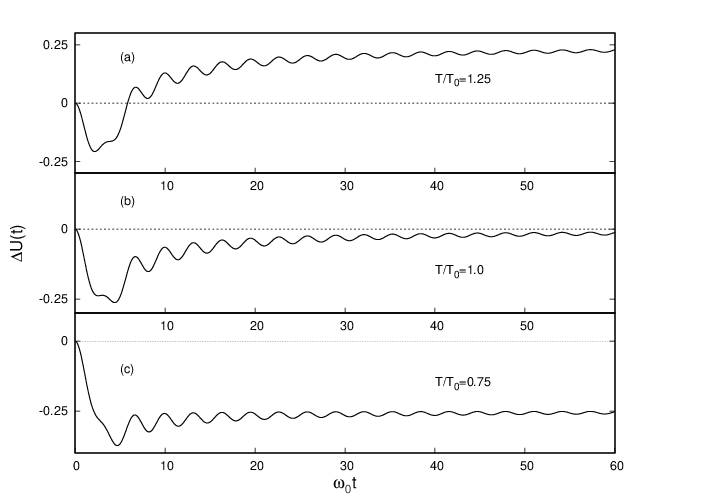
Substituting the above expressions for and into Eq. (144),
| (157) |
gives as an explicit function of time. Fig. 2 shows the result for three values of the temperature ratio . In all three cases, the energy change converges at long times to the value , which is consistent with the Clausius statement: the colder system absorbs heat from the hotter bath (), the hotter system releases heat into the colder bath (), and the net heat exchange is null when the temperatures of the system and bath are the same.
However, one observes from Fig. 2 that while the Clausius statement holds on the asymptotically long time scale, at short times it does not. The function is not monotonic; on short time intervals it increases/decreases regardless of whether the system hotter or colder than the bath. Such behavior is what was referred to as Scenario 1 in Introduction. In particular, one observes from Fig. 2 that regardless of the sign of the temperature difference the system initially loses energy: the function first decreases, reaches an absolute minimum, and then on a much longer time scale approaches non-monotonically the equilibrium value from below. Such an initial transient cooling (the term is suggested by the referee) may be interpreted as a result of the initial energy transfer from the system to the boundary atom of the bath. The latter is initially fixed, see Fig. 1, and immediately after being released at it is always “colder” than the system, even if the bath’s temperature is higher than that of the system. The net energy balance results from the interplay of two processes. The first process is the system releasing heat to to the colder boundary atom, the second process is the system absorbing heat from the hotter bath. The initial transient cooling may be viewed as the result that the first process dominates on a shorter time scale. The second process dominates on the longer time scale, and one expects the transient cooling to be more conspicuous when the second process is weaker, i.e. when the temperature of the bath is lower. This trend is visible in Fig. 2: for a fixed initial temperature of the system , the extent of the initial transient cooling increases when the temperature of the bath decreases. Instead, at higher one expects the transient cooling to be unimportant. Indeed, plotting according to Eq. (157) one finds that the initial transient cooling is practically invisible for .
XII Heat transfer for non-ergodic system (, )
As discussed in Sec. X, for and the system shows non-ergodic behavior due to formation of the localized vibrational mode. The resolvent is given by Eq. (152), . At long times the function vanishes, and the resolvent oscillates
| (158) |
with the amplitude and frequency given by Eqs. (153). The functions and , given by Eqs. (138), take the forms
| (159) | |||||
| (160) |
The time averages of these expressions, which we denote with the overbar, are
| (161) |
Taking into account that and , see Eqs. (153) and (40), we can express the above expressions as functions of the mass ratio as follows
| (162) |
The plots of the functions and , as well as another relevant function defined below, are shown in Fig. 3.
According to Eq. (137), the time-average change of the system’s internal energy is
| (163) |
The direction of the time-average heat transfer is determined by the sign of this expression. The heat transfer is anomalously directed (non-Clausius) if when the system is initially colder than bath (), or if when the system is initially hotter than bath (). It is easy to see that the latter case actually does not occur for the present model. Indeed, the inequality can be written as
| (164) |
If , it has no solutions because for any the left-hand side is negative and the right-hand side is positive (note that and , see Fig. 3). Thus, if the system is initially hotter than the bath, the heat transfer is in agreement with the Clausius statement, i.e. is directed from the hotter system to colder bath.

The situation is more interesting when the system is initially colder than the bath, . For that case the Clausius statement suggests that the system absorbs heat from the bath, so that . However, solving the inequality
| (165) |
one finds that the Clausius transfer only occurs if the system’s initial temperature is not too high, namely
| (166) |
where the function is
| (167) |
For the function monotonically decreases from from to at asymptotically large , see Fig. 3. Therefore, for any the critical temperature is lower than temperature of the bath, but bounded from below by the half-temperature of the bath,
| (168) |
If the initial temperature of the system is in the interval
| (169) |
then one finds
| (170) |
which corresponds to the non-Clausius heat transfer from the initially colder system to hotter bath. The anomalous heat transfer from the system to bath also occurs when their temperatures are the same, in which case .
These results may be interpreted as follows. Due to the formation of a localized vibrational mode, the system exchanges heat not with the entirety of the bath, but only with a finite fragment of the bath adjacent to the system. Suppose one wishes to introduce an effective local temperature of that fragment. Clearly, it must be lower than the bath’s bulk temperature because the fragment includes the initially frozen boundary atom . It is tempting to identify the fragment’s effective temperature with the critical temperature defined by (166). Then our results indicate that the Clausius statement breaks down when applied to the whole bath, yet is still valid when applied to the heat exchange between the system and the boundary fragment of the bath provided the latter has an effective temperature : Heat is transferred from the system to the fragment if the system’s temperature is higher than temperature of the fragment (though perhaps lower than the bulk temperature of the bath ), and in the opposite direction otherwise.
XIII Heat transfer for non-ergodic system ()
In the previous two sections we discussed the model for , which shows both ergodic (for ) and non-ergodic (for ) behavior. The condition of non-ergodicity implies that the isotope representing the system is at least twice lighter than atoms of the bath. In contrast, for a localized mode emerges, and the system is non-ergodic, for any value of the mass ratio , including the Brownian limit . This peculiar feature is the incentive to consider the case in this section as our second showcase example. We shall see, however, that the results for are qualitatively similar to those for the case discussed in the previous section.
We have seen in Sec. V that for the memory kernel in the Langevin equation takes a simple form, . However, this simplicity does not offer any particular advantage for the evaluation of the resolvent . The general expression for the resolvent’s transform (145) for reads
| (171) |
and cannot be inverted in terms of standard functions. One has to be aware of a subtlety related to this expression: If one tries to evaluate the long time limit of the resolvent using the final value theorem one gets zero,
| (172) |
which suggests ergodicity. Actually, result (172) is incorrect because, as we shall see, the long-time limit of the function with transform (171) for any positive does not exist, and the final value theorem cannot be applied.
The inversion of transform (171) is discussed in detail in Appendix B. It is similar to that for the case , but also involves some peculiar details. As was mentioned above, the inversion is not a merely mathematical exercise because the function has two branches, and one has to be careful to chose a physically meaningful branch. Function (171) has four simple poles, but only two of them are on the physical branch. Those two are located on the imaginary axis and have the form where
| (173) |
For any value of the mass ratio , the frequency is higher than and thus lies outside the spectrum of the bath’s normal modes. This is just the condition of the localized mode formation. The detailed calculation (see Appendix B) gives for the resolvent the result structurally similar to the one for the case
| (174) |
where the function is now defined by the integral
| (175) |
As for the case , at long times vanishes, and the resolvent oscillates with the frequency given by (173) and the amplitude
| (176) |
The internal energy change of the system also oscillates at long times. Its time average is given by the same expression (163) as for the case ,
| (177) |
where the time-averaged functions and are still given by Eqs. (161). For the squared internal frequency of the system is , and
| (178) |
Substituting this and Eq. (176) for into Eqs. (162) yields for and as explicit functions of the following expressions
| (179) |
While these expressions are different than those for the case , the qualitative behavior of functions and in two cases is similar, see Fig. 3, except that the functions domain in the present case is instead of .
Repeating the analysis of Section XII, i.e. solving inequalities and for different signs of the temperature difference , one finds results similar to the case . Namely, if the system is initially hotter than the bath , then the heat transfer is normal, i.e. the system loses energy, . On the other hand, one finds that the system may lose energy even if it is initially colder than the bath,
| (180) |
i.e. the heat transfer may be non-Clausius, provided the system temperature is higher than a critical temperature ,
| (181) |
Solving inequality (180), one finds for the critical temperature the expression with
| (182) |
The function behaves in a way qualitatively similar to that for the case , i.e. it monotonically decreases from to . Thus, we find for the critical temperature the same lower bound as for the case .
Similar to the case , we can interpret the results arguing that the boundary region of the bath is characterized by the effective temperature . Since is lower than the bath’s bulk temperature , a non-Clausius heat transfer from the colder system to hotter bath can be interpreted as a Clausius transfer from the system to the bath’s boundary region when the former is hotter than the latter.
XIV Conclusion
Thermodynamics is a macroscopic theory, and at present there is no consensus on to what extent and under what conditions it can be extended to microscopic and mesoscopic systems. Quoting Ref. IO: The conclusions of thermodynamics apply to macroscopic systems only. A system with small number of particles will not obey the laws of thermodynamics, especially the second law. Nevertheless, many efforts and progress have been made in recent years in constructing thermodynamics of small systems strongly coupled to the environment Gelin; Seifert; Jar; Talkner. In this paper we have followed a somewhat opposite route studying conditions when properties of microscopic open systems may be at odds with macroscopic thermodynamics.
We found that the second law in the form of the Clausius statement (heat does not spontaneously flow from cold to hot) does not generally hold, yet it is quite robust. For ergodic systems we found that the Clausius statement may be violated on microscopically short time intervals, yet it still holds on a coarse-grained time scale with a sufficiently low (“macroscopic”) time resolution. In particular, if one measures heat transfer for a transition with initial and final states being equilibrium ones (which means that the transition occurs on a time scale longer than the thermalization time of the system), the Clausius statement is valid and in agreement with other forms of the second law. The violation of the Clausius statement on a time scale shorter than the thermalization time involves the system out of equilibrium and does not contradict the second law in the form of the Clausius inequality, since the latter refers to transitions with initial and final states (but not necessarily intermediate states) being equilibrium ones.
Perhaps a more interesting result is that the Clausius statement may not hold in any sense for a non-ergodic system, which does not reach thermal equilibrium with the bath due to the formation of a localized vibrational mode. Again, this finding by no means compromises macroscopic thermodynamics, which concerns ergodic systems only. Still, we believe that the result is of interest as a concrete example which shows limitations of the (simple) thermodynamic description of a (complex) dynamical process of heat transfer involving small systems. Specifically, we found that the anomalously directed heat transfer from a cold non-ergodic system with initial temperature to a hotter bath with temperature occurs if the system temperature is higher than a certain critical temperature ,
| (183) |
This suggests to interpret as an effective temperature of a fragment of the bath adjacent to the system and involved in a localized vibrational motion. That fragment, in the studied setup, is effectively cooler than the rest of the bath because the boundary atom is initially fixed. Then our results are naturally accounted for by the assumption that the Clausius statement is still valid if we replace the bulk temperature of the bath by the bath’s local temperature at the boundary: Although the system is colder than the bath, , in the presence of a localized vibrational mode the system effectively interacts only with a bath’s small boundary region with the effective temperature . Then the system releases heat into the boundary region if , and absorbs heat from the region if .
The value of depends on parameters of the model and , but in all considered cases it is found to be bounded from below by the half-temperature of the bath, .
A simpler model of Ref. Plyukhin, where the system acquires the equilibrium distribution instantaneously, shows a similar behavior, but the result in that case is reversed in the sense that an anomalously directed heat transfer occurs from a colder bath to a hotter non-ergodic system (instead of from a colder system to a hotter bath in the present model).
In view of these findings, it is natural to ask whether the protocol studied here can be used to design a perpetual motion machine of the second kind. It is clear that one can use the set up with a non-ergodic system (e.g. when , or when to transfer some (small) amount of energy from a colder system to a hotter one. However, in order to arrange such transfer in a systematic way, we need to return the overall system into the initial configuration, depicted in Fig. 1, with the boundary atom fixed at the position corresponding to the mechanical equilibrium of the chain. Physically, a periodic protocol can be arranged by trapping the boundary atom in an external potential well, which can turned on and off in proper moments. This, however, appears to be impossible without some Maxwell’s demon-like apparatus.
As a technical tool, we derived and exploited the generalized Langevin equation (42) with a non-stationary noise. The non-stationarity of the noise reflects the non-stationarity of the heat transfer in the studied setting. The fluctuation-dissipation relation we found, see Eq. (90), differs from the standard one by the presence of additional terms involving not only the dissipative kernel, but also the kernel’s first derivative. Although the forms of the Langevin equation and fluctuation-dissipation relation used in this paper are model-sensitive, we believe they may be of interest as a simple example of the Langevin dynamics extended beyond the standard assumptions.
Although the linearity of the presented model is essential for all calculations, we believe that qualitatively our findings are not specific for linear systems only, in particular, because a non-ergodic behavior, similar to that considered here, is known to occur in nonlinear systems as well Dhar.
APPENDIX A: Derivation of Langevin equation for the boundary atom
In this appendix we derive the generalized Langevin equations (25) for the boundary atom .
According to Eq. (22), the equation of motion of the boundary atom is that of an oscillator linearly coupled to the system and also to normal mode oscillators of the bath,
| (A1) |
The right part of Fig. 1 gives a pertinent illustration. Normal mode coordinates satisfy Eq. (24),
| (A2) |
which has the general solution
| (A3) |
Here is a solution of the corresponding homogeneous equation
| (A4) |
Physically, describes evolution of normal modes when the boundary atom is fixed, . Integrating the second term in Eq. (A3) by parts and taking into account that , one gets
| (A5) |
Substitution of this expression into Eq. (A1) gives the generalized Langevin equation
| (A6) |
with the fluctuating force
| (A7) |
and the memory kernel
| (A8) |
Eqs. (A6)-(A8) are exact and hold for any . They take a more compact form for the infinite bath, . As follows from Eqs. (14) and (20),
| (A9) |
then one observes that
| (A10) |
Therefore, in the limit the Langevin equation (A6) takes the form
| (A11) |
which is just Eq. (25) of the main text.
APPENDIX B: Evaluation of resolvent for the case
In this Appendix we present the inversion of the Laplace transform (171)
| (B1) |
of the resolvent for the case and arbitrary positive .
Function (B1) has two branches which we denote and and write as
| (B2) |
where and are the two branches of the square-root function
| (B3) |
It is convenient to define a branch cut as a segment of the imaginary axis connecting the branch points , and to define in a polar form,
| (B4) |
see Fig. 4. Then the two branches of can be defined by the following expressions:
| (B5) |
where the ranges of arguments and for the first branch are the same,
| (B6) |
while for the second branch the range of is shifted by ,
| (B7) |
One can verify that the functions and defined in this way are continuous at any except on the branch cut. In what follows we shall need to refer to the following mapping rules for the functions and :
(a) Let with be on the positive imaginary axis above the branch cut. Then the first branch has a positive imaginary part, while the second branch has a negative imaginary part.
(b) Let with be on the negative imaginary axis below the branch cut. Then the first branch has a negative imaginary part, while the second branch has a positive imaginary part.
(c) Let be real and positive. Then the first branch is also real and positive, while the second branch is real and negative.
(d) Let be real and negative. Then the first branch is real and negative, while the second branch is real and positive.
With these preparations done, let us return to the function given by Eq. (B1). It has two branch points and four simple poles. Two of the poles are on the imaginary axes
| (B8) |
and another two are on the real axis
| (B9) |
Let us show that the pure imaginary poles (B8) are on the first branch , and real poles (B9) are on the second branch . According to (B1), each pole is a root of the equation
| (B10) |
for one of the two branches of the function . Let us determine for each pole the corresponding branch of and .
(1) At the pole Eq. (B10) gives for a pure imaginary value with a positive imaginary part. According to mapping rule (a), in this case must be represented by the branch . Therefore, the pole is on the resolvent’s first branch for any .
(2) At the pole Eq. (B10) gives for a pure imaginary value with a negative imaginary part. According to mapping rule (b), in this case must be again represented by the branch , and the pole is on the resolvent’s first branch for any .
(3) At the pole Eq. (B10) gives for a real negative value. According to mapping rule (c), in this case . The pole is on the second branch for any .
(4) At the pole Eq. (B10) gives for a real positive value. According to mapping rule (d), . The pole is on the second branch .
As the next step, we need to determine which of the two branches of the function is physically meaningful. Interestingly, this task is more involved compared to the case . Consider, for instance, the condition . Using the initial value theorem it can be written as
| (B11) |
One observes that this asymptotic relation is valid for both branches of and as goes to infinity along any directions of both real and imaginary axes of the complex plane. Instead of the initial condition for the resolvent, we can use that for the memory kernel, , see Eq. (51). For the transform of the kernel is given by Eq. (49),
| (B12) |
Then the initial value theorem requires
| (B13) |
Suppose goes to infinity, say, along the positive direction of the real axis. Then, according to the mapping rules (c), condition (B13) is only satisfied if the function is represented by its first branch . The same conclusion we arrive at when goes to zero along other directions. Thus, the physical branch of is the one involving the first branch of the square-root function . Since , the same is true about the resolvent. Therefore, the resolvent has to be found as the inversion of , i.e. as a Bromwich integral
| (B14) |
As discussed above, has two branch points and two simple poles with . Since all four singular points are on the imaginary axis, the integral (B14) is over an arbitrary vertical line to the right of the origin ( is real and positive).

The evaluation of integral (B14) is an exercise of the standard technique based on Cauchy’s residue theorem. First, consider the auxiliary integral
| (B15) |
over the closed contour shown at the right part of Fig. 4. Here we use the notation for a residue of a function at . One can show that contributions to the integral from the large arc (of radius ) and small circles (of radius ) about branch points both go to zero when and . The contribution from the two horizontal lines along the negative real axis is also zero when the distance between the lines vanishes because the integrand is continuous on the -axis. The only non-zero contributions to are those from the two vertical segments along the branch cut () and from the vertical segment of the length on the right (), . In the limit the integral equals , therefore , and
| (B16) |
The integral has two contributions . Consider first the contribution from the vertical path just left from the branch cut, i.e. from to . Using the path parametrization
| (B17) |
we can write in the form
| (B18) |
As follows from Eq. (B6), on the given path for the first branch and , and therefore
| (B19) |
Also, it is easy to figure out that for the given path . Then
| (B20) |
Then integral takes the form
| (B21) |
Separating real and imaginary parts of the fraction yields
| (B22) |
In a similar way, using the path parametrization
| (B23) |
one evaluates the second contribution from the vertical path just right from the branch cut,
| (B24) |
Here the negative sign reflects that the path is directed downward. According to Eq. (B6), on the given path for the first branch and , therefore
| (B25) |
and
| (B26) |
As for , it is convenient to separate real and imaginary parts of the fraction,
| (B27) |
Adding up Eqs. (B22) and (B27), and taking into account that the contribution from the odd part of the integrand is zero, one finds
| (B28) |
The next step is to evaluate the residues in expression (B16). One can verify that the poles are of the first order, then
| (B29) |
Using the L’Hospital’s rule one gets
| (B30) |
According to mapping rule (a)
| (B31) |
Then
| (B32) |
The second pole at is evaluated in a similar way, so we get
| (B33) |
Finally, the substitution of expressions (B28) for and (B33) for the residues into Eq. (B16) yields
| (B34) |
Here the term
| (B35) |
can be shown to vanish in the limit , and the amplitude and frequency of the oscillatory term are
| (B36) |
Although it is not immediately obvious, one can verify numerically that the result (B34) satisfies the correct initial condition .
References
- (1) V. Capek and D. P. Sheehan, Challenges to The Second Law of Thermodynamics, Springer, Dordrecht (2005).
- (2) R. Clausius, The Mechanical Theory of Heat, London. Macmillan and Co. (1879).
- (3) C. Jarzynski and D. K. Wójcik, Classical and quantum fluctuation theorem for heat exchange, Phys. Rev. Lett. 92, 230602 (2004).
- (4) D. H. E. Gross and J. F. Kenney, The microcanonical thermodynamics of finite systems: The microscopic origin of condensation and phase separations, and the conditions for heat flow from lower to higher temperatures, J. Chem. Phys. 122, 224111 (2005).
- (5) S. Hilbert, P. Hänggi, and J. Dunkel, Thermodynamic laws in isolated systems, Phys. Rev. E 90, 062116 (2014).
- (6) P. Hänggi, S. Hilbert, and J. Dunkel, Meaning of temperature in different thermostatistical ensembles, Phil. Trans. R. Soc. A 374, 20150039 (2016).
- (7) R. H. Swendsen, Thermodynamics of finite systems: a key issues review, Rep. Prog. Phys. 81, 072001 (2018).
- (8) J.-X. Hou, Violation of the temperature-signifies-heat-flow rule in systems with long-range interactions, Phys. Rev. E 99, 052114 (2019).
- (9) K. Micadei, J. P. S. Peterson, A. M. Souza, R. S. Sarthour, I. S. Oliveira, G. T. Landi, T. B. Batalhao, R. M. Serra, and E. Lutz, Reversing the direction of heat flow using quantum correlations, Nature Commun. 10, 2456 (2019).
- (10) A.V. Plyukhin, Non-Clausius heat transfer: the example of harmonic chain with an impurity, J. Stat. Mech. 063212 (2020).
- (11) P. Mazur and I. Oppenheim, Molecular theory of Brownian motion, Physica 50, 241 (1970).
- (12) J.-E. Shea and I. Oppenheim, Fokker-Planck equation and Langevin equation for one Brownian particle in a nonequilibrium bath, J. Phys. Chem. 100, 19035 (1996).
- (13) M. G. McPhie, P. J. Daivis, I. K. Snook, J. Ennis, and D. J. Evans, Generalized Langevin equation for nonequilibrium systems, Physica A 299, 412 (2001).
- (14) R. Hernandez and F. L. Somer, Stochastic Dynamics in Irreversible Nonequilibrium Environments. 1. The Fluctuation-Dissipation Relation, J. Phys. Chem. B 103, 1064 (1999).
- (15) M. Vogt and R. Hernandez, An idealized model for nonequilibrium dynamics in molecular systems, J. Chem. Phys. 123, 144109 (2005).
- (16) S. Kawai and T. Komatsuzaki, Derivation of the generalized Langevin equation in nonstationary environments, J. Chem. Phys. 134, 114523 (2011).
- (17) B. Cui and A. Zaccone, Generalized Langevin equation and fluctuation-dissipation theorem for particle-bath systems in external oscillating fields, Phys. Rev. E 97, 060102(R) (2018).
- (18) H. Meyer, T. Voigtmann, and T. Schilling, On the non-stationary generalized Langevin equation, J. Chem. Phys. 147, 214110 (2017).
- (19) P. Bohec, F. Gallet, C. Maes, S. Safaverdi, P. Visco and F.Van Wijland, Probing active forces via a fluctuation-dissipation relation, Eur. Phys. Lett. 102, 50005 (2013).
- (20) C. Maes, On the second fluctuation–dissipation theorem for nonequilibrium baths, J. Stat. Phys. 154, 705 (2014).
- (21) U. Weiss, Quantum Dissipative Systems, World Scientific, Singapore (2008).
- (22) Hänggi P, Generalized Langevin equations: A useful tool for the perplexed modeller of nonequilibrium fluctuations? Lecture Notes in Physics 484, 15 (1997).
- (23) J. T. Hynes, Transient initial condition effects for Brownian particle motion, J. Chem. Phys. 59, 3459 (1973).
- (24) J. T. Hynes, Initial condition effects for a Brownian particle in a harmonic chain, J. Stat. Phys. 11, 257 (1974).
- (25) W. Bez, Microscopic preparation and macroscopic motion of a Brownian particle, Z. Phys. B 39, 319 (1980).
- (26) L. Debnath, The double Laplace transforms and their properties with applications to functional, integral and partial differential equations, Int. J. Appl. Comput. Math 2, 223-241 (2016).
- (27) E. W. Montroll and R. B. Potts, Effect of defects on lattice vibrations, Phys. Rev. 100, 525 (1958).
- (28) R. Rubin, Momentum autocorrelation functions and energy transport in harmonic crystals containing isotopic defects, Phys. Rev. 131, 964 (1963).
- (29) T. Morita and H. Mori, Kinetic and hydrodynamic scalings in an exactly-solvable model of the Brownian motion, Prog. Theor. Phys. 56, 499-514 (1976).
- (30) I. Oppenheim, Entropy, information, and the arrow of time, J. Phys. Chem. B 114, 16184 (2010).
- (31) M. F. Gelin and M. Thoss, Thermodynamics of a subensemble of a canonical ensemble, Phys. Rev. E 79, 051121 (2009).
- (32) U. Seifert, First and second laws of thermodynamics at strong coupling, Phys. Rev. Lett. 116, 020601 (2016).
- (33) C. Jarzynski, Stochastic and macroscopic thermodynamics of strongly couples systems, Phys. Rev. X 7, 011008 (2017).
- (34) P. Talkner and P. Hänggi, Statistical mechanics and thermodynamics at strong coupling: Quantum and classical, Rev. Mod. Phys. 92, 041002 (2020).
- (35) A. Dhar and K. Wagh, Equilibration problem for the generalized Langevin equation, EPL 79, 60003 (2007).