Generating a topological anomalous Hall effect in a non-magnetic conductor

Introduction. The ordinary Hall effect occurs in a classical magnetic field due to the Lorentz force and has been well understood since its discovery. In contrast, the understanding of the anomalous Hall effect (AHE) has been a key challenge for modern physics Nagaosa et al. 2010. Originally observed in ferromagnets, it was shown to exist in paramagnetic materials as well Culcer et al. 2003. The origins, relative importance and even existence of the manifold contributions to the AHE have spawned a debate spanning three quarters of a century Luttinger 1958; Smit 1958; Berger 1970; Nozières and Lewiner 1973; Crépieux and Bruno 2001; Dugaev et al. 2001; Onoda and Nagaosa 2002; Culcer et al. 2003; Haldane 2004; Sinitsyn et al. 2007; Inoue et al. 2006; Onoda et al. 2008; Sinitsyn 2008; Kovalev et al. 2009; Nagaosa et al. 2010; Yang et al. 2011; Nomura and Nagaosa 2011. Fittingly, controversy surrounds it even as it opens new avenues of research Culcer and Das Sarma 2011; Ado et al. 2015; A. Ado et al. 2017; Liu et al. 2018a; Keser et al. 2019; Yang et al. 2019.

The band-structure or intrinsic contribution to the AHE, nowadays understood to stem from the Berry curvature and have a topological origin, is quantized under certain circumstancesOnoda and Nagaosa 2002; Culcer et al. 2003; Haldane 2004; Sinitsyn et al. 2007; Yu et al. 2010; Chang et al. 2013; Chang et al. 2015; Bestwick et al. 2015; Qi et al. 2016; Liu et al. 2016. This places it in the expanding category of quantized topological responses, which include the quantum Hall and quantum spin-Hall effects Klitzing et al. 1980; Bernevig et al. 2006; König et al. 2007; Culcer et al. 2020. Notably, quantized responses have only been observed in systems that are effectively one-dimensional, being intimately connected with the existence of edge states König et al. 2007; Chang et al. 2013; Chang et al. 2015; Bestwick et al. 2015; Collins et al. 2018. Whereas the intrinsic AHE can be quantized in a two-dimensional semiconductor, such quantization is impossible to observe in practice, since (i) the dispersion involves an even number of Zeeman-split Kramers pairs that make opposite topological contributions, yielding a non-universal conductivity that is often density-dependent Jungwirth et al. 2002; Nunner et al. 2007; Sinitsyn et al. 2007; Nagaosa et al. 2010 and (ii) disorder corrections are very strong Inoue et al. 2006; Culcer et al. 2017. Nevertheless, we show here that, with appropriate design, the Berry curvature can be unambiguously identified in 2D transport even when the response is not quantized.

We show that a Hall effect can be generated in a two-dimensional heavy-hole system grown on a low-symmetry substrate when an in-plane magnetic field $B_{\parallel}$ is applied. In the absence of an out-of-plane magnetic field and therefore of a Lorentz force, there is no ordinary Hall effect. Instead, an anomalous Hall effect occurs due to the finite Berry curvature of the spin-3/2 hole system, with no counterpart in spin-1/2 electron systems. The gap in the dispersion that enables the Hall response is opened by a shear Zeeman term in the Lande $g$-tensor Yeoh et al. 2014; Li and Sushkov 2016. Our central result is the Hall conductivity $\sigma_{xy}$ linear in $B_{\parallel}$, shown in Figs. 1 and 2 and expected from the Onsager relations. We refer to this phenomenon as the anomalous planar Hall effect (APHE). Its origins are intrinsic and topological: we show that neither scalar nor extrinsic spin-orbit scattering contribute to leading order in $B_{\parallel}$. The APHE is a manifestation of relativistic quantum mechanics in classical transport mediated by topological terms in the crystal band structure, which reflect inter-band coherence induced by external electromagnetic fields. Since the equilibrium system is not magnetized the effect is tunable in situ by altering the magnetic field orientation. It is observable in state-of-the-art hole samples, which are developing at a brisk pace, motivated in part by quantum computing applications Nichele et al. 2014a; Nichele et al. 2014b; Brauns et al. 2016a; Brauns et al. 2016b; Wang et al. 2016; Akhgar et al. 2016; Qu et al. 2016; Nichele et al. 2017a; Srinivasan et al. 2017; Conesa-Boj et al. 2017; Li et al. 2017; Li et al. 2018; Vukusic et al. 2018; Liles et al. 2018; Hendrickx et al. 2018; Crippa et al. 2018; Hendrickx et al. 2020; Marx et al. 2020, where holes are actively investigated Kloeffel et al. 2013; Shim and Tahan 2014; Hung et al. 2017, by their large spin-orbit coupling Moriya et al. 2014; Nichele et al. 2017b; Beukman et al. 2017, interesting transport properties Liu et al. 2014; Liu et al. 2018b; Marcellina et al. 2018; Marcellina et al. 2020; Samanta et al. 2020, and by unconventional properties stemming from their spin-3/2 nature Winkler et al. 2008; Liu et al. 2008; Chesi et al. 2011; Scholz et al. 2013; Sacksteder and Bernevig 2014; Biswas and Ghosh 2014; Mawrie et al. 2014; Cuan and Diago-Cisneros 2015; Fu and Egues 2015; Biswas et al. 2015; Wenk et al. 2016; Mawrie et al. 2017; Liang and Lyanda-Geller 2017; Bladwell and Sushkov 2019.

We consider a two-dimensional hole gas grown along (113). Our findings hold for a multitude of low-symmetry growth directions, and (113) is chosen as an example. The ground state is represented by the heavy hole manifold, where heavy holes have spin projection $\pm 3/2$ onto the quantization axis, which is perpendicular to the plane. At normal transport densities the light hole manifold is not occupied. Our results are obtained using the Luttinger Hamiltonian rotated along the growth direction (113) with the vertical confinement modeled by the Bastard wave-function, given in the Supplement. Nevertheless, the underlying physics can be understood from the effective Hamiltonian for the lowest heavy hole sub-band $H_{hh}=\varepsilon_{0{\bm{k}}}+H_{s}+H_{c}$, where $\varepsilon_{0{\bm{k}}}=\hbar^{2}k^{2}/(2m^{*})$, with $m^{*}$ the heavy-hole in-plane effective mass and ${\bm{k}}$ the in-plane wave vector. The term $H_{s}=(\hbar/2){\bm{\sigma}}\cdot{\bm{\Omega}}_{\bm{k}}$, with ${\bm{\sigma}}$ the vector of Pauli spin matrices, captures the leading contributions to the Rashba and Zeeman effects, which stem from the spherical terms in the Luttinger Hamiltonian Winkler 2000; Winkler et al. 2002; Winkler 2003; Durnev et al. 2014; Marcellina et al. 2017; Miserev and Sushkov 2017; Miserev et al. 2017, as well as the out-of-plane Zeeman term, which stems from the cubic symmetry of diamond and zincblende lattices Li and Sushkov 2016. These can be incorporated into an effective field ${\bm{\Omega}}_{\bm{k}}$. We assume $\Omega_{F}\tau\gg 1$, with $\Omega_{F}$ the value of ${\bm{\Omega}}_{\bm{k}}$ on the Fermi surface and $\tau$ the momentum relaxation time. Written in full,

with $\alpha$ is the Rashba spin-orbit constant in the spherical approximation, $k_{\pm}=k_{x}\pm ik_{y}$, $B_{\pm}=B_{x}\pm iB_{y}$, and $\Delta_{1},\Delta_{2},\Delta_{3},\Delta_{4}$ are effective Lande $g$-factors, with $\Delta_{3},\Delta_{4}$ only present in asymmetric wells Miserev and Sushkov 2017; Miserev et al. 2017. The shear Zeeman term $\Delta_{zx}\sigma_{z}B_{x}$ is vital Yeoh et al. 2014; Li and Sushkov 2016, yielding an out-of-plane Zeeman splitting in response to an in-plane magnetic field that, henceforth, we assume to be $\parallel\hat{\bm{x}}$, where $\hat{\bm{x}}\parallel(33\bar{2})$. The eigenvalues of $H_{0}+H_{s}$ are $\varepsilon_{{\bm{k}}\pm}=\varepsilon_{0{\bm{k}}}\pm\hbar|\Omega_{\bm{k}}|$. Cubic symmetry leads to the following additional spin-orbit terms

Here $\eta_{1}$ has contributions from the Dresselhaus terms $\propto C_{D},B_{D1}$ in Ref. Marcellina et al. 2017, $\eta_{2}\propto B_{D1}$, while $\eta_{3}$ and $\eta_{4}$ have contributions from both Dresselhaus and cubic-symmetry terms. We recall that Dresselhaus terms are absent in diamond lattices such as Si and Ge, but are noticeable in zincblende materials such as GaAs and InAs.

We focus first on the Hall current due to $H_{s}$, which provides the dominant contribution. The effect of the much smaller terms contained in $H_{c}$ Marcellina et al. 2017, as well as disorder, is discussed in the closing section. The Zeeman term for heavy holes also includes terms $\propto B_{\parallel}^{3}$, yet these are three orders of magnitude smaller than the $B_{\parallel}-$linear terms above, only becoming important for $B_{\parallel}\geq 30$ T. The coefficients in Eqs. 1, 2 are functions of $k$ and decrease strongly at larger wave vectors. Such momentum-dependent Zeeman terms with different winding numbers are likewise specific to heavy holes, since these correspond to the $\pm 3/2$ projection of the hole spin-$3/2$ onto the quantization axis Marcellina et al. 2020. They have no counterpart in electron systems. In our evaluations this $k$-dependence is circumvented by using the full Luttinger Hamiltonian.

Unlike the ordinary Hall effect driven by the Lorentz force, the charge dynamics here originate in the spin locking to the wave vector. As a hole is accelerated longitudinally its wave vector changes and it experiences a different spin-orbit field. As a result of this the spin undergoes a rotation, which in turn produces a change in the wave vector that is perpendicular to the longitudinal motion, in other words, a Hall current. The intrinsic Hall conductivity, derived below, is given by $\sigma_{xy}^{0}=-\frac{e^{2}}{h}\int d^{2}k/(2\pi)\,{\mathcal{F}}_{z}^{n}$, where the Berry curvature of sub-band $n$ is $\bm{\mathcal{F}}_{n}=-{\rm Im}\,\langle\partial u_{n}/\partial{\bf k}|\times|\partial u_{n}/\partial{\bf k}\rangle$, with $u_{n}$ the lattice-periodic Bloch wave function, whose role is played here by the envelope function. The full effect as a function of magnetic field, including its material dependence, is shown in Fig. 1 for a symmetric well and in Fig. 2 for a strongly asymmetric well, in which the Rashba interaction dominates. The form and behaviour of the Hall conductivity are understood by noting that (i) the shear Zeeman term opens a gap, which makes the Berry curvature nonzero; (ii) the spin-split bands have different Fermi wave vectors, and (iii) the sign of the Berry curvature is determined by the winding direction of the spin-orbit field ${\bm{\Omega}}_{\bm{k}}$, with the Rashba, in-plane Zeeman and the Dresselhaus terms all yielding the same sign. However, for different low symmetry growth directions these contributions can yield different signs. We first provide a pedagogical analytical explanation for these two limiting cases: a symmetric well with a single in-plane Zeeman term expected to dominate at small densities, and a strongly asymmetric well. For simplicity we use constant coefficients to derive approximate analytical expressions for $\sigma_{xy}$, noting that this pedagogical approach is restricted to very small densities and magnetic fields. The dispersions for these two cases are sketched in Fig. 3.

In a symmetric well in Si and Ge, given that there is no a-priori spin-orbit coupling, the Berry curvature is initially zero. When the in-plane magnetic field is applied, the Zeeman terms $\propto\Delta_{1},\Delta_{2}$, give rise to a non-zero Berry curvature at each ${\bm{k}}$, while the Zeeman term $\propto\Delta_{zx}$ opens a gap in the spectrum. Interestingly the Berry curvature itself is independent of $B_{\parallel}$, although it depends explicitly on the in-plane and out-of-plane $g$-factors. Since the heavy-hole sub-band is now spin-split by the out-of-plane Zeeman interaction there are two different Fermi wave vectors. The difference between them is linear in the magnetic field at low fields, as shown in the Supplement, hence the conductivity is linear in $B_{\parallel}$. With only the $\Delta_{1}$ and $\Delta_{zx}$ terms, the Hall conductivity reads

which increases monotonically with $B_{\parallel}$. In GaAs and InAs, on the other hand, the Dresselhaus terms cause $\sigma_{xy}$ to be non linear at small fields but their contribution to the Berry curvature is eventually overwhelmed by the in-plane Zeeman terms as $B_{\parallel}$ increases.

In an asymmetric well the Berry curvature is likewise zero in the absence of the out-of-plane Zeeman interaction. Nevertheless, the heavy hole sub-band is already spin-split by the strong Rashba spin-orbit interaction even before the magnetic field is turned on, so that there is a sizable difference between the two Fermi wave vectors. The Rashba interaction overwhelms all other terms, as shown recently Marcellina et al. 2017, hence the plots for the asymmetric well increase monotonically for all materials. When the Zeeman term $\propto\Delta_{zx}$ opens a gap a significant Hall current emerges. With only the Rashba and $\Delta_{zx}$ terms, the Hall conductivity takes the form

The Fermi wave vectors $k_{F\pm}\approx(\frac{2m^{*}\epsilon_{F}}{\hbar^{2}}\pm\frac{4\sqrt[6]{54}\alpha m^{*\frac{5}{2}}\epsilon_{F}^{\frac{3}{2}}}{\hbar^{5}})^{1/2}$ differ due to the Rashba interaction, while their magnetic field dependence is negligible. Because of this, when the spin-orbit energy $\Omega_{F}>\Delta_{zx}B_{x}$ but is still much less than the kinetic energy, $\sigma_{xy}$ is approximately independent of spin-orbit strength. This insight is more general than just the Rashba case, and explains the relative smallness of the effect and its comparable size in all materials studied. The APHE is driven by the cubic-symmetry and bulk Zeeman terms, which are strongest in InAs and Ge. In a realistic sample we expect $\rho_{xy}\sim 100-500\mu\Omega$.

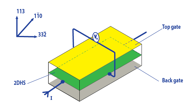
Experimental measurement. A schematic of an experimental setup that could be used to measure the APHE is shown in Fig. 4. To identify the topological terms experimentally, one can start with a (113) QW with a top and bottom gate that enables full control of the Rashba interaction Papadakis et al. 1999; Li et al. 2016; Yeoh et al. 2014, and apply an in-plane magnetic field to introduce the Zeeman interactions 1. The topological terms can be detected through the Hall voltage, since it depends directly on $\sigma_{xy}$. As the magnetic field is rotated in the plane the Hall current will disappear, since $\Delta_{zy}=0$, enabling one to turn the APHE on and off in situ. As the field is rotated out of the plane the APHE will give way to the ordinary Hall effect.

Methodology. The full Hamiltonian $H=\varepsilon_{0{\bm{k}}}+H_{s}+H_{E}+U$. The driving electric field ${\bm{E}}\parallel\hat{\bm{y}}$ is contained in $H_{E}=e{\bm{E}}\cdot\hat{\bm{r}}$. The scattering potential $U({\bm{r}})=\sum_{I}\bar{U}({\bm{r}}-{\bm{R}}_{I}),$ includes both scalar and extrinsic spin-orbit scattering Bi et al. 2013, where ${\bm{R}}_{I}$ indexes the random locations of impurities, and the scattering potential due to a single impurity is denoted by $\bar{U}({\bm{r}})$. In Fourier space, $\bar{U}_{{\bm{k}}{\bm{k}}^{\prime}}=\mathcal{U}_{{\bm{k}}{\bm{k}}^{\prime}}\openone+\mathcal{V}_{{\bm{k}}{\bm{k}}^{\prime}}$, where $\mathcal{U}_{{\bm{k}}{\bm{k}}^{\prime}}$ represents a matrix element between plane waves, and, $\mathcal{V}_{{\bm{k}}{\bm{k}}^{\prime}}=-\frac{i\lambda}{2}\,{\bm{\sigma}}\cdot({\bm{\omega}}_{\bm{k}}\times{\bm{k}}^{\prime}-{\bm{\omega}}_{{\bm{k}}^{\prime}}\times{\bm{k}})\,\mathcal{U}_{{\bm{k}}{\bm{k}}^{\prime}}$ where ${\bm{\omega}}_{{\bm{k}}}=k^{3}\,(\cos 3\theta,\sin 3\theta,0)$, assuming $\lambda k_{F}^{4}\ll 1$. Since the Rashba Hamiltonian is derived from the Luttinger Hamiltonian in the spherical approximation it has the same form along (113) as along (001), and thus the extrinsic spin-orbit scattering term has the same form as in Ref. Bi et al. 2013. As written in the Pauli basis, the spin dependent term $\mathcal{V}_{{\bm{k}}{\bm{k}}^{\prime}}$ points out of the plane. We note that $\lambda$ for holes has not been determined quantitatively. We consider short-range scattering off uncorrelated impurities, with the average of $\langle{\bm{k}}n|\hat{U}|{\bm{k}}^{\prime}n^{\prime}\rangle\langle{\bm{k}}^{\prime}n^{\prime}\hat{U}|{\bm{k}}n\rangle$ over impurity configurations $n_{i}|\bar{U}_{{\bm{k}}{\bm{k}}^{\prime}}^{nn^{\prime}}|^{2}/V$, where $n_{i}$ is the impurity density and $V$ the crystal volume.

We derive a quantum kinetic equation as described in Refs. Culcer et al. 2017; Vasko and Raichev 2005. The density matrix $\rho$ is found in the basis $\{{\bm{k}}n\}$, where $n$ represents the band index. To determine the charge current we require $f_{\bm{k}}$, the part of the density matrix diagonal in wave vector, since the current operator is diagonal in ${\bm{k}}$. From the quantum Liouville equation, $\partial\rho/\partial t+(i/\hbar)\,[H,\rho]=0$, we obtain the following kinetic equation describing the time evolution of $f_{\bm{k}}$:

where the scattering term in the Born approximation

and the driving term $\mathcal{D}_{E,{\bm{k}}}=\frac{Df_{0{\bm{k}}}}{D{\bm{k}}}$. The covariant derivative $\frac{Df_{0{\bm{k}}}}{D{\bm{k}}}=\frac{\partial f_{0{\bm{k}}}}{\partial{\bm{k}}}-i\,[\mathcal{\bm{R}}_{\bm{k}},f_{0{\bm{k}}}]$ arises from the ${\bm{k}}$-dependence of the basis functions. The Berry connection matrix elements $\mathcal{\bm{R}}_{\bm{k}}^{mm^{\prime}}=\langle u_{\bm{k}}^{m}|i\frac{\partial u_{\bm{k}}^{m^{\prime}}}{\partial{\bm{k}}}\rangle$, with $m\neq m^{\prime}$ necessarily, are interband matrix elements of the position operator, which also appear in the current density operator ${\bm{j}}=-(e/\hbar)\,DH_{0{\bm{k}}}/D{\bm{k}}$. In an external electric field one may decompose $f_{\bm{k}}=f_{0{\bm{k}}}+f_{E{\bm{k}}}$, where $f_{0{\bm{k}}}$ is the equilibrium density matrix and $f_{E{\bm{k}}}$ is a correction to first order in the electric field. The equilibrium density matrix is $f_{0{\bm{k}}}=(1/2)\,[(f_{{\bm{k}}+}+f_{{\bm{k}}-})\openone+\tilde{\sigma}_{z}(f_{{\bm{k}}+}-f_{{\bm{k}}-})]$, where $f_{{\bm{k}}\pm}$ represent the Fermi-Dirac distributions over subband energies $\varepsilon_{{\bm{k}}\pm}$, and the tilde in $\tilde{\sigma}_{z}$ denotes the basis of eigenstates of the band Hamiltonian. In linear response one may replace $f_{{\bm{k}}}\rightarrow f_{0{\bm{k}}}$ in the driving term $\mathcal{D}_{E,{\bm{k}}}$. With $f_{0{\bm{k}}}$ known and $\mathcal{D}_{E,{\bm{k}}}$ on the right-hand side of Eq. (5), we obtain $f_{E{\bm{k}}}$. By taking the trace with the current operator, the longitudinal and transverse components of the current are found. The off-diagonal part of the density matrix contains the intrinsic term $S_{E{\bm{k}}}^{mm^{\prime}}=-i\hbar\mathcal{P}[D^{mm^{\prime}}_{E{\bm{k}}}(\varepsilon^{m}_{\bm{k}}-\varepsilon^{m^{\prime}}_{\bm{k}})]$, with $\mathcal{P}$ the principal part, and this yields directly the intrinsic Hall conductivity as introduced above.

Disorder contributions. Disorder is responsible for a complex series of contributions to the Hall conductivity, which in related models tend to reduce the Hall effect or cancel it altogether Inoue et al. 2006; Culcer et al. 2017. Disorder contributions fall into two categories: those stemming from scalar disorder and from spin-dependent disorder. The former exist because of inter-band coherence induced by the electric field, which causes even scalar disorder to contribute to the Hall effect through an anomalous driving term

Here we have singled out the band-diagonal term in the density matrix, $n_{E{\bm{k}}}^{mm^{\prime}}\propto\delta^{mm^{\prime}}$. To find $D^{\prime\,mm^{\prime\prime}}_{E{\bm{k}}}$, we first solve for $n_{E{\bm{k}}}$, feed it into the scattering term Eq. 6, and take the band off-diagonal part. When calculated explicitly this contribution is identically zero for both symmetric and strongly asymmetric wells for both the spherical Rashba interaction and the Zeeman terms.

The spin-dependent disorder term $\mathcal{V}_{{\bm{k}}{\bm{k}}^{\prime}}$ gives rise to four different contributions: skew scattering, side-jump, anomalous spin precession and the anomalous scattering term. These were described in detail in Ref. Bi et al. 2013 for the spin-Hall effect, and the method we follow here is exactly analogous. Due to the large winding numbers involved the anomalous spin precession and the anomalous scattering terms are zero for holes, while skew scattering and side-jump contribute only to order $B_{\parallel}^{3}$. We also find the contribution from $J_{\lambda}(S_{E\parallel})$ to be imaginary. Hence, with the Rashba interaction evaluated in the spherical approximation, and in the absence of Dresselhaus terms there are no disorder contributions to the APHE.

We investigate next the additional contributions to the Hall current due to the Dresselhaus and cubic-symmetry Rashba term. The term $\propto\eta_{3}$ in Eq. 2 is linear in wave vector, therefore their contribution to the intrinsic part of the Hall current is cancelled exactly by the scalar disorder term in the same way as the customary linear Rashba term in electron systems Inoue et al. 2006; Culcer et al. 2017. It does not contribute to the extrinsic signal because they generate a spin-orbit field that is purely in the plane. The Dresselhaus terms make a contribution to the Berry curvature, which is noticeable only in a symmetric wells, as discussed above. Since the Dresselhaus spin-orbit field $\propto\eta_{1},\eta_{2}$ points entirely out of the plane, it does not contribute to the extrinsic signal through the anomalous scattering term $J_{\Omega\lambda}(n_{E\parallel})$. It does not contribute to the Hall current through the anomalous driving term either. The only way a nonzero contribution to the current can emerge is through products of the Dresselhaus terms and cubic symmetry terms, which will then be multiplied by the small parameter $\lambda k_{F}^{4}\ll 1$. Therefore, in Si and Ge the extrinsic contribution to the APHE vanishes altogether, while in InAs and GaAs it is negligibly small.

In summary, we have shown that low-symmetry growth hole nanostructures exhibit a purely Berry-curvature driven Hall effect in response to an in-plane magnetic field. The APHE may open new pathways in the electrical operation of spin qubits and spin-orbit torques.