Detecting Hierarchical Changes
in Latent Variable Models

Shintaro Fukushima Affiliation: Graduate School of Information Science and Technology
The University of Tokyo, Tokyo, Japan
Email: sfukushim@gmail.com Kenji Yamanishi Affiliation: Graduate School of Information Science and Technology
The University of Tokyo, Tokyo, Japan
Email: yamanishi@g.ecc.u-tokyo.ac.jp

Abstract

This paper addresses the issue of detecting hierarchical changes in latent variable models (HCDL) from data streams. There are three different levels of changes for latent variable models: 1) the first level is the change in data distribution for fixed latent variables, 2) the second one is that in the distribution over latent variables, and 3) the third one is that in the number of latent variables. It is important to detect these changes because we can analyze the causes of changes by identifying which level a change comes from (change interpretability). This paper proposes an information-theoretic framework for detecting changes of the three levels in a hierarchical way. The key idea to realize it is to employ the MDL (minimum description length) change statistics for measuring the degree of change, in combination with DNML (decomposed normalized maximum likelihood) code-length calculation. We give a theoretical basis for making reliable alarms for changes. Focusing on stochastic block models, we employ synthetic and benchmark datasets to empirically demonstrate the effectiveness of our framework in terms of change interpretability as well as change detection.

Index Terms:

Change detection, Latent variable model, Hierarchical change detection, Data stream, Minimum description length principle

I Introduction

I-A Motivation

We are concerned with the issue of detecting changes in latent variable models. In the areas of knowledge discovery and data mining, latent variable models play a central role with various applications, such as stochastic block model (SBM) [1] for networks, latent Dirichlet allocation (LDA) [2] for texts, and Gaussian mixture model (GMM) for numeric data. Let us consider network change detection problem, for example. Conventionally, this problem has been considered on the basis of the (quasi-) difference between probability distributions (e.g., [3, 4]). In other words, if the distance between the distributions before any given point and that after the point is significantly large, then we consider the point as a change point. Spectral information such as eigenvectors of the association matrix may be employed instead of the distribution difference (e.g., [5, 6, 7]). However, it is not clearly understood where the change comes from with such methods. Actually, there are several levels in network changes. Let us consider a time-evolving SBM [1, 8] as an example. 1) On the first level of changes, the connection between the nodes changes. 2) On the second level, a block distribution changes. 3) On the third level, the number of blocks or community organization changes. We say that the level is higher in the order of 1) $<$ 2) $<$ 3). Even if we detect change points with distance-based or spectrum-based methods, we can not identify which level the change comes from due to the complex nature of networks.

However, it is important to know the levels of the changes. The main reason is that we can interpret the cause of a change by looking at its level. For example, 1) corresponds to a change in degrees of communication between nodes. 2) corresponds to a change in community distribution. 3) corresponds to a drastic change in community organization. The level of severity of change is in the order of 3) $>$ 2), 1). We call this problem of identifying the causes of changes the interpretability problem. Note that when 3) occurs, changes in degrees of communication between nodes and community distribution occur consequently. We distinguish this case from 1) and 2), where community organization does not change.

Another reason is that when changes at a higher level occur gradually, we can detect signs of the changes by detecting changes at lower levels. For example, the detection of changes at levels 1) and 2) may lead to early signals of changes at level 3). We call this the change sign detection problem.

The above argument is valid for general classes of latent variable models as shown in Fig. 1. 1) corresponds to the data distribution change for a fixed latent variable, 2) corresponds to the change of latent variables for a fixed number of blocks, and 3) corresponds to the change of the number of latent variables.

Fig. 1: Hierarchical changes in latent variable models.

The primary purpose of this paper is to propose a framework in which we do not only detect changes in latent variable models but also identify their levels in a hierarchical way. We name this framework hierarchical change detection for latent variable models (HCDL). We present a theory for making reliable alarms of changes in a hierarchical way. We also focus on SBM to experimentally demonstrate the effectiveness of HCDL, in terms of change level identification as well as change detection.

I-B Novelty and Significance

The novelty and significance of this study are summarized as follows:

1) A novel framework for hierarchical change detection. Our HCDL framework is novel in its ability to detect changes at different levels: distribution, latent variable, and model. For SBM, these correspond to individual communication level, community distribution one, and community organization one, respectively. This enables us to identify the cause of any change and to interpret the meaning of the change.

Our framework is designed from an information-theoretic viewpoint based on the minimum description length (MDL) principle [9, 10]. That is, learning and change detection are conducted by finding the probability distributions with the shortest description lengths. The key idea of our framework is to combine the MDL change statistics[11, 12] with the DNML (decomposed normalized maximum likelihood) code-length[13, 14] calculation method in change scoring for latent variable models. First, we employ the MDL change statistics to score the degree of change at any given time point. It measures how much the data can be compressed by changing the model at that time point. In the original MDL change statistics, NML code-length [10] has been employed to calculate code-lengths. When a latent variable model is considered, however, hierarchical changes can not be detected if we simply apply the NML code-length. This is because the NML code-length can not be decomposed for data and latent variables. Thus, we propose to use the DNML code-length instead of the NML code-length. Therefore, we can identify from which level any change comes.

2) Theoretical basis for making reliable alarms. The test for changes based on the MDL change statistics with DNML code-length is referred to as the MDL test throughout this study. In order to make reliable alarms for the MDL test, we need to determine the threshold for change scores at respective levels. We theoretically derive upper bounds on Type I and Type II error probabilities for the MDL test and thereby design the thresholds for scores so that Type I error probability (false alarm rate) is properly upper bounded. The thresholds are determined for all levels (distribution, latent variable, and model). Hence, we could raise alarms of hierarchical changes for which the reliability is theoretically guaranteed.

3) Novel analysis of hierarchical changes in terms of change interpretation and change sign detection. Through HCDL, we offer two new methodologies for analyzing change detection. One is hierarchical interpretation of detected changes. With HCDL, we can not only detect the changes but also identify from which level the changes come from. Changes may simultaneously originate from different levels. Then, we can quantitatively analyze how much the individual changes contribute to the overall one. This yields a new approach to interpretation of changes. The other methodology is change sign detection. Suppose that a change occurs gradually. Then, we expect that changes at lower levels may occur before those at higher ones. For example, in the case of network change detection, changes in network connections among given communities or those of the community distribution may be signs of a more drastic community structure change. We conduct experiments with synthetic and real datasets to demonstrate the effectiveness of change detection at respective levels, hierarchical interpretability, and change sign detection with HCDL.

I-C Related Work

The issue of change detection in latent variable models such as network models has been explored extensively in the areas of knowledge discovery and data mining (e.g., [15, 16, 17] ). Most of previous studies were concerned with detection of parameter changes in data distributions. Such studies often employed distribution-difference-based or spectrum-based methods, as in Section I-A. However, these methods can not deal with changes at higher levels such as structural changes. Hence, the different levels of changes can not be identified. Therefore, these approaches lack interpretability of changes. Some previous studies were concerned with the issue of dynamic model selection [18]. See also related notions such as tracking best experts [19] and switching distributions [20]. Some previous studies were concerned with the issue of dynamic model selection[18]. Time-evolving networks [21] and Graphscope [22] dealt with topics related to dynamic model selection (see also the survey [23] in community detection in dynamic networks). That is, Their goal is to detect changes in discrete structures, the number of clusters, and the number of communities at higher levels. However, among such studies, there was no attempt to identify changes at lower levels as well as those of higher ones.

The main target of conventional studies on change detection was abrupt change. Recently, gradual change [11] has become a new target of change detection. Incremental changes have also been discussed in the scenario of concept drifts [24]. It is a challenging new problem: how can we detect signs of changes when they are gradual or incremental? There are a number of studies on model change sign detection [25, 26, 27, 28, 29]. However, the change signs studied there have not been related to changes at different levels; therefore, the causes of changes in signs can not be explained.

II Problem Setting

In this section, we describe the problem setting of change detection in latent variable models. Let ${\mathcal{X}}$ be the data domain, which can be either continuous or discrete, and ${\mathcal{Z}}$ be the range of latent variables, which is finite. Let $X\in{\mathcal{X}}$ and $Z\in{\mathcal{Z}}$ be random variables, and $x$ and $z$ denote their realizations, respectively. We denote $x_{a}^{b}=x_{a}\dots x_{b}$ . When $a=1$ , we write $x_{1}^{b}$ as $x^{b}$ . We write $x_{1}^{b}$ as $x^{b}$ .

Let ${\mathcal{M}}$ be the set of discrete models, e.g., clusters and communities. Suppose that each datum $(x_{t},z_{t})$ at time $t$ is independently drawn from a probability density (or mass) function of a latent variable model of the following general form:

\displaystyle(x_{t},z_{t})\sim f(X,Z;\theta,M),

(1)

where $M\in\mathcal{M}$ is a model. The probability density (or mass) function in Eq. (1) is assumed to be factorized as

\displaystyle f(X,Z;\theta,M)=f(X|Z;\theta_{1},M)f(Z;\theta_{2},M),

(2)

where $\theta=(\theta_{1},\theta_{2})$ , $\theta_{1}$ is the real-valued parameter of probability density function of observed variables given latent variables, while $\theta_{2}$ is the real-valued parameter of the probability mass function of latent variables. In the case of SBM, $X$ is a data matrix, $Z$ is the block assignment of each data, $\theta_{1}$ is an edge weight parameter, $\theta_{2}$ is a parameter of block distribution, and $M$ is a structure indicating the number of blocks.

We are concerned with detecting the three levels in changes:

•

Level 1: Change of parameter $\theta_{1}$ of data distribution for fixed latent variables. It means an inner-level change in the probabilistic model for $X$ for given $Z$ . For example, changes in connections within a community in SBM belong to level 1.
•

Level 2: Change of parameter $\theta_{2}$ of latent variable distribution. It means a change in the probabilistic model for $Z$ . For example, community distribution change in SBM belongs to level 2.
•

Level 3: Change of model M. It means a drastic structural change in the probabilistic model for $X$ and $Z$ . For example, change in the number of communities or community organization in SBM belongs to level 3.

Our target issues are summarized as follows:

1.

How can we detect changes at each level accurately?
2.

How can we interpret the detected changes by relating them to their levels?
3.

How can we find signs of changes at higher levels by detecting changes at lower levels?

We address these issues using the HCDL framework.

III Information Theoretic Methods for Change Detection

We take an information-theoretic approach to change detection on the basis of the MDL principle. That is, we detect a change point by finding a time point so that the total code-length required for encoding the data and its distribution is shortest. Two key notions to realize the hierarchical change detection for latent variable models are the MDL change statistics and the DNML code-length. We effectively combine these two notions in our HCDL framework. In this section, we focus on the issue of detecting changes at level 3 in order to clarify the information-theoretic methodology.

III-A MDL Change Statistics

The MDL change statistics [12, 11] is a score that measures the degree of change for a specified time point $t$ within a given window. Let $t$ be a given time point. Prepare a window of size $2h$ whose center is $t$ ( $h\in\mathbb{N})$ . The MDL change statistics at time $t$ , which we denote as $\Phi_{t}$ , is defined as the difference between the total code-length required for encoding the data with an unchanged model and that with models changed before and after time $t$ . It is formally defined as follows:

Definition III.1.

(MDL change statistics) For a fixed window size $2h\in\mathbb{N}$ , let ${\bm{x}}_{(t)}=x_{t-h+1}^{t+h}$ , ${\bm{x}}_{(t)}^{-}=x_{t-h+1}^{t}$ , ${\bm{x}}_{(t)}^{+}=x_{t+1}^{t+h}$ . Similarly, ${\bm{z}}_{(t)},{\bm{z}}^{+}_{(t)},{\bm{z}}^{-}_{(t)}$ are defined. The MDL change statistics $\Phi_{t}$ is defined as

$\displaystyle\Phi_{t}$	$\displaystyle=\frac{1}{2h}\min_{M}\left\{L({\bm{x}}_{(t)},{\bm{z}}_{(t)};M)+L(M)\right\}$	(3)
	$\displaystyle\quad-\frac{1}{2h}\min_{M_{1},M_{2}}\biggl\{L({\bm{x}}_{(t)}^{-},{\bm{z}}_{(t)}^{-};M_{1})+L({\bm{x}}_{(t)}^{+},{\bm{z}}_{(t)}^{+};M_{2})$
	$\displaystyle\quad\quad\quad\quad\quad\quad\quad+L(M_{1},M_{2})\biggr\}.$	(4)

Here, $L({\bm{x}},{\bm{z}};M)$ denotes the code-length for $({\bm{x}},{\bm{z}})$ relative to model $M$ . $L(M)$ is the code-length for model $M$ , whereas $L(M_{1},M_{2})$ is the code-length required for encoding model $M_{1}$ and $M_{2}$ .

The code-length $L(w)$ for $w$ means the length of codewords when $w$ is encoded into a binary sequence under the prefix condition that any codeword is not a prefix of any other ones. This condition holds if and only if Kraft’s inequality holds: $\sum_{w}2^{-L(w)}\leq 1$ , where the sum ranges over all possible $w$ s. Intuitively, the MDL change statistics measures the degree of change at time $t$ in terms of how much data is compressed by using different models before and after time $t$ . We describe how to calculate $L(M)$ and $L(M_{1},M_{2})$ in Section VI-A.

When a data stream is given, we slide the window to sequentially calculate Eq. (4). We thereby obtain a sequence of the MDL change statistics. By finding a time point when the MDL change statistics exceeds a threshold, we can find a change point of model $M$ , i.e., at level 3.

In the original definition of the MDL change statistics, the normalized maximum likelihood (NML) code-length is employed to calculate $L({\bm{x}},{\bm{z}};M)$ in it. It is formalized as

	$\displaystyle L_{{}_{\mathrm{NML}}}({\bm{x}},{\bm{z}};M)$	$\displaystyle=-\log f({\bm{x}},{\bm{z}};\hat{\theta}({\bm{x}},{\bm{z}}),M)$
		$\displaystyle\quad+\log\sum_{{\bm{x}}^{\prime},{\bm{z}}^{\prime}}f({\bm{x}}^{\prime},{\bm{z}}^{\prime};\hat{\theta}({\bm{x}}^{\prime},{\bm{z}}^{\prime}),M),$		(5)

where $\hat{\theta}({\bm{x}},{\bm{z}})$ is the maximum likelihood estimator of $\theta$ from $({\bm{x}},{\bm{z}})$ .

The problem in the NML code-length is that it can not be decomposed into the part of data and that of latent variables. It can not be decomposed into the part of data and that of latent variables. Hence, we can not identify the three levels of changes as in Section II if we simply employ the NML code-length in the MDL change statistics.

III-B DNML Code-Length

In order to resolve the problem in the previous section, we employ the decomposed normalized maximum likelihood (DNML) code-length for latent variable models instead of the NML code-length. In calculating the DNML code-length, the total code-length is decomposed into the sum of the NML code-length for data conditioned on latent variables and that for the latent variables. According to [14, 13], it is formulated as follows:

Definition III.2.

(DNML code-length) [14, 13] The DNML code-length for $(x,z)$ for a model $M$ is defined as

\displaystyle L_{{}_{\mathrm{DNML}}}(x,z;M)\mathrel{\overset{\makebox[0.0pt]{\mbox{\tiny def}}}{=}}L_{{}_{\mathrm{NML}}}(x|z;M)+L_{{}_{\mathrm{NML}}}(z;M),

(6)

where

	$\displaystyle L_{{}_{\mathrm{NML}}}(x\|z;M)$	$\displaystyle=-\log{f(x\|z;\hat{\theta}_{1}(x,z);M)}+\log{C_{X\|z}(M)},$		(7)
	$\displaystyle L_{{}_{\mathrm{NML}}}(z;M)$	$\displaystyle=-\log{f(z;\hat{\theta}_{2}(z),M)}+\log{C_{Z}(M)}.$

Here, $\hat{\theta}_{1}$ and $\hat{\theta}_{2}$ are the maximum likelihood estimators of $\theta_{1}$ and $\theta_{2}$ as in Eq. (2), and

	$\displaystyle C_{X\|z}(M)$	$\displaystyle\mathrel{\overset{\makebox[0.0pt]{\mbox{\tiny def}}}{=}}\sum_{x}f(x\|z;\hat{\theta}_{1}(x,z),M),$		(8)
	$\displaystyle C_{Z}(M)$	$\displaystyle\mathrel{\overset{\makebox[0.0pt]{\mbox{\tiny def}}}{=}}\sum_{z}f(z;\hat{\theta}_{2}(z),M).$		(9)

According to [14, 13], it is known that $C_{X|z}(M)$ and $C_{Z}(M)$ are efficiently computable in order $O(n+|{\mathcal{M}}|)$ for a wide range of classes of latent variable models such as SBM, LDA, and GMM.

Theorem III.1.

(DNML for SBM) SBM is a canonical model for community detection [1]. SBM partitions the vertices of a network into groups. We assume that every group has its own probability to generate a link. A model $M$ denotes a structure of partitioning.

According to [13], the DNML code-length $L_{{}_{\mathrm{DNML}}}(x,z;M)$ for SBM is calculated as follows:

$\displaystyle L_{{}_{\mathrm{DNML}}}(x,z;M)$	$\displaystyle=\sum_{k_{1}}\sum_{k_{2}}\left(n_{k_{1}k_{2}}\log{n_{k_{1}k_{2}}}\right.$
	$\displaystyle\quad\quad\quad\left.-n_{k_{1}k_{2}}^{+}\log{n_{k_{1}k_{2}}^{+}}-n_{k_{1}k_{2}}^{-}\log{n_{k_{1}k_{2}}^{-}}\right)$
	$\displaystyle\quad+\sum_{k_{1}}\sum_{k_{2}}\log{C(n_{k_{1}k_{2}},2)}$
	$\displaystyle\quad+\sum_{k}n_{k}(\log{n}-\log{n_{k}})+\log{C(n,K)},$	(10)

where $n_{k_{1}k_{2}}^{+}$ and $n_{k_{1}k_{2}}^{-}$ are the number of links and no-links in group $(k_{1},k_{2})$ . $n_{k_{1}k_{2}}$ is defined as $n_{k_{1}k_{2}}=n_{k_{1}k_{2}}^{+}+n_{k_{1}k_{2}}^{-}$ , which is the total number of links in group $(k_{1},k_{2})$ . $\log{C(n,K)}$ is the normalization term $C_{Z}$ as in Equation (9) for data of length $n$ following the multinomial distribution with $K$ elements.

Since $z$ is not observable, we may instead employ the estimator of $\hat{z}(x)$ from $x$ instead of $z$ . As an estimator, for example, we may employ the one that maximizes the posterior probability estimated by the Expectation-Maximization (EM) algorithm.

In the following, we denote $\bm{x}_{(t)}=x_{t-h+1}^{t+h}$ , $\bm{x}^{-}_{(t)}=x_{t-h+1}^{t}$ , $\bm{x}^{+}_{(t)}=x_{t+1}^{t+h}$ . Similarly, $\bm{z}_{(t)}$ , $\bm{z}^{-}_{(t)}$ , and $\bm{z}^{+}_{(t)}$ are defined likewise. The DNML can be applied to model selection [14]. That is, the DNML model estimator $\hat{M}_{t}$ from $({\bm{x}}_{(t)},{\bm{z}}_{(t)})$ at time $t$ is given by

\displaystyle\hat{M}_{t}=\operatornamewithlimits{argmin}_{M}\{L_{{}_{\mathrm{DNML}}}({\bm{x}}_{(t)},\hat{{\bm{z}}}_{(t)};M)+L(M)\},

(11)

where $L(M)$ denotes the code-length for model $M$ , and $L_{{}_{\mathrm{DNML}}}(\bm{x}_{(t)},\bm{z}_{(t)};M)$ is calculated as the sum of DNML code lengths in the window:

\displaystyle L_{{}_{\mathrm{DNML}}}(\bm{x}_{(t)},\bm{z}_{(t)};M)

\displaystyle=\sum_{\tau=t-h+1}^{t+h}L_{{}_{\mathrm{DNML}}}(x_{\tau},z_{\tau};M),

(12)

where $\hat{\theta}_{1}$ and $\hat{\theta}_{2}$ are estimated to minimize the log-likelihoods:

	$\displaystyle\hat{\theta}_{1}(\bm{x}_{(t)},\bm{z}_{(t)})$	$\displaystyle=\operatornamewithlimits{argmin}_{\theta_{1}}\sum_{\tau=t-h+1}^{t+h}-\log{f(x_{\tau}\|z_{\tau};\theta_{1},M)},$		(13)
	$\displaystyle\hat{\theta}_{2}(\bm{z}_{(t)})$	$\displaystyle=\operatornamewithlimits{argmin}_{\theta_{2}}\sum_{\tau=t-h+1}^{t+h}-\log{f(z_{\tau};\theta_{2},M)}.$		(14)

Plugging the DNML formula in Eq. (6) into the formula of the MDL change statistics yields the MDL change statistics combined with DNML as follows:

$\displaystyle\Phi_{t}$	$\displaystyle=\frac{1}{2h}\min_{M}\left\{L_{{}_{\mathrm{DNML}}}({\bm{x}}_{(t)},{\bm{z}}_{(t)};M)+L(M)\right\}$
	$\displaystyle\quad-\frac{1}{2h}\min_{M_{1},M_{2}}\left\{L_{{}_{\mathrm{DNML}}}({\bm{x}}_{(t)}^{-},{\bm{z}}_{(t)}^{-};M_{1})\right.$
	$\displaystyle\quad\quad\left.+L_{{}_{\mathrm{DNML}}}({\bm{x}}_{(t)}^{+},{\bm{z}}_{(t)}^{+};M_{2})+L(M_{1},M_{2})\right\}.$	(15)

By sliding the window, for a threshold parameter $\epsilon>0$ , we determine that a model change occurred if $\Phi_{t}>\epsilon$ and that it did not, otherwise. We call this test the MDL test. Once the model change is detected, we can identify the model with Eq. (11).

IV Theory for Making Reliable Alarms

IV-A Error Probabilities for Change Detection

We need to choose a threshold parameter $\epsilon$ for the MDL change statistics in order to make reliable alarms. to make reliable alarms. For this purpose, we first present a theoretical property of the MDL change statistics in terms of error probabilities in the scenario of hypothesis testing. We then derive the threshold so that the error probabilities are properly bounded. We continue to focus on the change detection of level 3, i.e., model change detection.

Let us consider the following hypothesis testing. For a time point $t$ , the null hypothesis $H_{0}$ is that no model change occurs at time $t$ , while the alternative hypothesis $H_{1}$ is that it occurs at time $t$ . Here, we do not know anything about model $M$ .

	$\displaystyle H_{0}$	$\displaystyle:({\bm{x}}_{(t)},{\bm{z}}_{(t)})\sim f(X^{2h},Z^{2h};\theta^{\ast}_{0},M^{\ast}_{0}),$
	$\displaystyle H_{1}$	$\displaystyle:({\bm{x}}^{-}_{(t)},{\bm{z}}_{(t)}^{-})\sim f(X^{h},Z^{h};\theta^{\ast}_{1},M^{\ast}_{1}),$
		$\displaystyle\quad({\bm{x}}^{+}_{(t)},{\bm{z}}_{(t)}^{+})\sim f(X^{h},Z^{h};\theta^{\ast}_{2},M^{\ast}_{2}),$

where $M^{\ast}_{0}$ , $M^{\ast}_{1}$ , and $M^{\ast}_{2}$ ( $M^{\ast}_{1}\neq M^{\ast}_{2}$ ) are the unknown true models, and $\theta^{\ast}_{0}$ , $\theta^{\ast}_{1}$ , and $\theta^{\ast}_{2}$ are the unknown true values of the parameters.

We conduct the hypothesis testing using the MDL test as follows: we accept $H_{1}$ if $\Phi_{t}>\epsilon$ for $\Phi_{t}$ as in Eq. (III-B); otherwise, we accept $H_{0}$ . We evaluate this test in terms of Type I and II error probabilities. For the Type I error probability, $H_{0}$ is true, but $H_{1}$ is accepted by the MDL test. Meanwhile, for the Type II error probability, $H_{1}$ is true, but $H_{0}$ is accepted by the MDL test. We have the following theorem on the MDL test for model changes.

Theorem IV.1.

The Type I error probability $\delta_{1}$ and Type II error probability $\delta_{2}$ for the MDL test with $\Phi_{t}$ in Eq. (III-B) are given as follows:

		$\displaystyle\delta_{1}\leq\exp{\left\{-2h\left(\epsilon-\frac{\log{C(M_{0}^{\ast})}+L(M_{0}^{\ast})}{2h}\right)\right\}},$		(16)
		$\displaystyle\delta_{2}\leq\exp{\left\{-n\left(d({f}_{{}_{\mathrm{NML}}},f_{M_{1\ast 2}})-\frac{\ell(M_{1}^{\ast},M_{2}^{\ast},\epsilon)}{2n}\right)\right\}},$		(17)

where

		$\displaystyle\log{C(M)}\mathrel{\overset{\makebox[0.0pt]{\mbox{\tiny def}}}{=}}\log{C_{X\|Z}(M)C_{Z}(M)},\,C_{X\|Z}(M)\mathrel{\overset{\makebox[0.0pt]{\mbox{\tiny def}}}{=}}\max_{{\bm{z}}}C_{X\|{\bm{z}}},$
		$\displaystyle\ell(M_{1}^{\ast},M_{2}^{\ast},\epsilon)\mathrel{\overset{\makebox[0.0pt]{\mbox{\tiny def}}}{=}}\log{C(M_{1}^{\ast})C(M_{2}^{\ast})}+L(M_{1}^{\ast},M_{2}^{\ast})+2h\epsilon,$
		$\displaystyle d(f_{{}_{\mathrm{NML}}},f_{M_{1\ast 2}})$
		$\displaystyle\mathrel{\overset{\makebox[0.0pt]{\mbox{\tiny def}}}{=}}-\frac{1}{n}\log\sum_{{\bm{x}}_{(t)},{\bm{z}}_{(t)}}\left(f_{{}_{\mathrm{NML}}}({\bm{x}}_{(t)},{\bm{z}}_{(t)})f({\bm{x}}_{(t)},{\bm{z}}_{(t)};M_{1}\ast M_{2})\right)^{\frac{1}{2}},$
		$\displaystyle f_{{}_{\mathrm{NML}}}({\bm{x}}_{(t)},{\bm{z}}_{(t)})\mathrel{\overset{\makebox[0.0pt]{\mbox{\tiny def}}}{=}}\frac{2^{-\min_{M}L_{{}_{\mathrm{NML}}}({\bm{x}}_{(t)},{\bm{z}}_{(t)};M)}}{\sum_{{\bm{x}},{\bm{z}}}2^{-\min_{M}L_{{}_{\mathrm{NML}}}({\bm{x}},{\bm{z}};M)}},$
		$\displaystyle f(\bm{x}_{(t)},\bm{z}_{(t)};M_{1}\ast M_{2})$
		$\displaystyle\mathrel{\overset{\makebox[0.0pt]{\mbox{\tiny def}}}{=}}f(\bm{x}_{(t)}^{-},\bm{z}_{(t)}^{-};\theta^{\ast}_{1},M_{1}^{\ast})f(\bm{x}_{(t)}^{+},\bm{z}_{(t)}^{+};\theta^{\ast}_{2},M_{2}^{\ast}).$

Theorem IV.1 can be proven by extending Theorem 3.1 in [12] to latent variable models. Theorem IV.1 shows that both Type I and II error probabilities for the MDL test with the DNML code-length converge to zero exponentially as the sample size increases if $\epsilon$ is properly designed. The rates of convergence depend on the information complexity of true models and the discrepancy measure of the probability distributions before and after the change.

IV-B Choosing Threshold Parameters

On the basis of the theory in the previous section, we show how to determine the threshold parameter $\epsilon$ to make a reliable alarm of a change. The key idea is to determine $\epsilon$ so that Type I error probability is upper-bounded by a predetermined confidence parameter. That is, letting a confidence parameter be $\delta>0$ , we choose $\epsilon$ so that the Type I error probability in Eq. (16) is upper-bounded by a confidence parameter $\delta$ . This implies that $\epsilon$ should satisfy the following inequality:

\displaystyle\epsilon\geq\frac{\log{C(M_{0}^{\ast})}+\log{L(M_{0}^{\ast})}-\log{\delta}}{2h}.

(18)

We use this criterion to choose $\epsilon$ for given $\delta$ in order to guarantee the reliability of an alarm. Since $\delta$ is a much smaller value than $\epsilon$ , the choice of $\delta$ does not affect the result compared to that of $\epsilon$ .

Note that the true model $M_{0}^{\ast}$ in Eq. (18) is not known in real cases. Hence, we estimate it as $\hat{M}_{t}$ in Eq. (11) and plug it into Eq. (18). We adopt the right-hand side value of Eq. (18) as $\epsilon$ .

V Hierarchical Change Detection

In Sections III and IV, we focused on detecting changes at level 3. This section extends the methodology into the hierarchical change detection for all three levels.

Let us denote $\hat{M}$ as the minimizer of the first term of the right-hand side of the MDL change statistics in Eq. (III-B), and $\hat{M}_{1},\hat{M}_{2}$ as the minimizers in the second term. In order to extend our discussion in previous sections into hierarchical change detection, we first note that $\Phi_{t}$ in Eq. (III-B) is decomposed as follows:

\displaystyle\Phi_{t}

\displaystyle=\Phi_{t}^{X|Z}+\Phi_{t}^{Z}+\Delta L_{t}(\hat{M},\hat{M}_{1},\hat{M}_{2}),

(19)

where

	$\displaystyle\Phi_{t}^{X\|Z}$	$\displaystyle\mathrel{\overset{\makebox[0.0pt]{\mbox{\tiny def}}}{=}}\frac{1}{2h}\left\{L_{{}_{\mathrm{NML}}}({\bm{x}}_{(t)}\|{\bm{z}}_{(t)};\hat{M})\right.$
		$\displaystyle\quad\quad\left.-(L_{{}_{\mathrm{NML}}}({\bm{x}}_{(t)}^{-}\|{\bm{z}}_{(t)}^{-};\hat{M}_{1})+L_{{}_{\mathrm{NML}}}({\bm{x}}_{(t)}^{+}\|{\bm{z}}_{(t)}^{+};\hat{M}_{2}))\right\},$
	$\displaystyle\Phi_{t}^{Z}$	$\displaystyle\mathrel{\overset{\makebox[0.0pt]{\mbox{\tiny def}}}{=}}\frac{1}{2h}\left\{L_{{}_{\mathrm{NML}}}({\bm{z}}_{(t)};\hat{M})\right.$
		$\displaystyle\quad\quad\left.-(L_{{}_{\mathrm{NML}}}({\bm{z}}_{(t)}^{-};\hat{M}_{1})+L_{{}_{\mathrm{NML}}}({\bm{z}}_{(t)}^{+};\hat{M}_{2}))\right\},$
	$\displaystyle\Delta L_{t}$	$\displaystyle\mathrel{\overset{\makebox[0.0pt]{\mbox{\tiny def}}}{=}}\frac{1}{2h}\left\{L(\hat{M})-L(\hat{M}_{1},\hat{M}_{2})\right\}.$

Eq. (19) means that the MDL change statistics can be decomposed into the sum of those for different levels. $\Phi_{t}^{X|Z}$ is the MDL change statistics for data $X$ given latent variable $Z$ , while $\Phi_{t}^{Z}$ is that for $Z$ itself. This decomposition owes to the nature of DNML code-length.

We can realize hierarchical change detection by making use of the property in Eq. (19) as follows: Let $\epsilon$ be a threshold parameter satisfying Eq. (18). If $\Phi_{t}>\epsilon$ , then we determine that a model change occurred, i.e., $\hat{M}\neq\hat{M}_{1}$ or $\hat{M}\neq\hat{M}_{2}$ . Otherwise, we determine that no model change occurred, i.e., $\hat{M}=\hat{M}_{1}=\hat{M}_{2}$ .

Then, we further investigate whether any change occurred at lower levels. Let $\epsilon_{{}_{X|Z}}>0$ and $\epsilon_{{}_{Z}}>0$ be threshold parameters. If $\Phi^{Z}_{t}>\epsilon_{{}_{Z}}$ holds, we determine that a change occurred in the distribution over latent variable $Z$ . Otherwise, we determine that such a change did not occur (level 2). Likewise, if $\Phi^{X|Z}_{t}>\epsilon_{{}_{X|Z}}$ , we determine that a change occurred with respect to observed variable $X$ for given latent variable $Z$ . Otherwise, we determine that such a change did not occur (level 1).

The threshold parameters $\epsilon_{{}_{X|Z}}$ and $\epsilon_{{}_{Z}}$ are determined similarly. That is, letting $\delta_{{}_{X|Z}}>0$ and $\delta_{{}_{Z}}>0$ be given confidence parameters, $\epsilon_{{}_{X|Z}}$ and $\epsilon_{{}_{Z}}$ are determined so that Type I error probability for the MDL test is upper-bounded by $\delta_{{}_{X|Z}}$ and $\delta_{{}_{Z}}$ , respectively. That is, for model $M$ , we have

\displaystyle\epsilon_{{}_{X|Z}}\geq\frac{\log{C_{X|Z}(M)}-\log{\delta_{{}_{X|Z}}}}{2h},\epsilon_{{}_{Z}}\geq\frac{\log{C_{Z}(M)}-\log{\delta_{{}_{Z}}}}{2h},

(20)

where $C_{X|Z}(M)$ and $C_{Z}(M)$ are as in Eq. (9).

Note that the severity of levels 1 and 2 can not be ordered linearly when changes at level 1 and 2 occur simultaneously, we can evaluate the importance of both, respectively, as follows:

\displaystyle w_{t}^{X|Z}

\displaystyle=\frac{\Phi_{t}^{X|Z}}{\Phi_{t}^{X|Z}+\Phi_{t}^{Z}},\quad w_{t}^{Z}=\frac{\Phi_{t}^{Z}}{\Phi_{t}^{X|Z}+\Phi_{t}^{Z}}.

(21)

Summarizing the above arguments, we show the core algorithm for HCDL in Algorithm 1. Through this algorithm, we can detect changes at different levels, thereby can interpret the causes of the changes by identifying their levels.

Algorithm 1 Hierarchical change detection algorithm for latent variable models (HCDL)

h

: window size,

\delta,\delta_{{}_{X|Z}},\delta_{{}_{Z}}

: parameters for controlling Type I error probabilities of model and parameter changes.

1: for

t=h,h+1,\,\dots

2: Calculate the MDL change statistics

\Phi_{t}

3: if

\Phi_{t}>\epsilon

then

4: Raise an alarm of change at level 3.

5: else

6: Estimate the model at

t

\hat{M}_{t}

according to Eq. (11).

7: Determine the threshold parameters

\epsilon_{{}_{X|Z}}

\epsilon_{{}_{Z}}

as in Eq. (20).

8: if

\Phi^{X|Z}_{t}>\epsilon_{{}_{X|Z}}

then

9: Raise an alarm of change at level 1.

10: end if

11: if

\Phi^{Z}_{t}>\epsilon_{{}_{Z}}

then

12: Raise an alarm of change at level 2.

13: end if

14: if

\Phi^{X|Z}_{t}>\epsilon_{{}_{X|Z}},\Phi^{Z}_{t}>\epsilon_{{}_{Z}}

then

15: Calculate the weights

w_{t}^{X|Z}

and

w_{t}^{Z}

of changes at levels 1 and 2 according to Eq. (21).

16: end if

17: end if

18: end for

VI Experiments

In this section, we conduct experiments with synthetic and real datasets to demonstrate the effectiveness of HCDL ¹¹ 1 Source codes are available at https://github.com/s-fuku/hcdl..

VI-A Synthetic Dataset 1 (Abrupt Change)

VI-A1 Dataset

For $t=1,\dots,80$ , we generated links $x_{t}$ between nodes as follows:

\displaystyle x_{t}\sim\begin{cases}\mathrm{SBM}\,(x_{t};\pi^{1},\theta^{1},K=3)&(t=1),\\ \mathrm{LinkTrans}\,(x_{t-1}|z_{t-1};\theta^{1},\beta)&(t=2,\dots,19),\\ \mathrm{SBM}\,(x_{t};\pi^{1},\theta^{2},K=3)&(t=20),\\ \mathrm{LinkTrans}\,(x_{t-1}|z_{t-1};\theta^{2},\beta)&(t=21,\dots,39),\\ \mathrm{SBM}\,(x_{t};\pi^{2},\theta^{2},K=3)&(t=40),\\ \mathrm{LinkTrans}\,(x_{t-1}|z_{t-1};\theta^{2},\beta)&(t=41,\dots,59),\\ \mathrm{SBM}\,(x_{t};\pi^{3},\theta^{3},K=4)&(t=60),\\ \mathrm{LinkTrans}\,(x_{t-1}|z_{t-1};\theta^{3},\beta)&(t=61,\dots,80),\end{cases}

(22)

where $\mathrm{SBM}\,(x;\pi,\theta,K)$ indicates that the model of SBM is $K$ , with the mixture probability $\pi=(\pi_{1},\dots,\pi_{K})$ , and the link probability $\theta=\{\theta_{k,\ell}\}_{k,\ell=1}^{K}$ . Here, $\pi^{1},\pi^{2}\in[0,1]^{3}$ , $\pi^{3}\in[0,1]^{4}$ , and $\theta^{1},\theta^{2}\in[0,1]^{3\times 3}$ , $\theta^{3}\in[0,1]^{4\times 4}$ . We denote $\pi^{i}=(\pi^{i}_{1},\dots,\pi^{i}_{K})$ $(i=1,2,3)$ and assume that $\pi_{i}^{1}\leq\dots\leq\pi_{i}^{K}$ . Likewise, we denote $\theta^{i}=\{\theta^{i}_{k,\ell}\}_{k,\ell=1}^{K}$ $(i=1,2,3)$ . $\mathrm{LinkTrans}(x|z;\theta,\beta)$ means that some links are regenerated according to $\theta$ for each combination of blocks with probability $\beta$ . In the following experiments, we set $\beta=0.02$ . The hyperparameter of $\pi^{1}$ was set to $\alpha=1$ (the Dirichlet distribution), and those of $\theta^{1}$ were set to $a=b=1$ (the Beta distribution). $\theta^{2}=\{\theta^{2}_{k,\ell}\}_{k,\ell=1}^{3}$ was set as follows:

\displaystyle\theta^{2}_{k,\ell}=\begin{cases}\theta^{1}_{k,\ell}+u&(0\leq\theta^{1}_{k,\ell}+u\leq 1),\\ 1-\epsilon&(\theta^{1}_{k,\ell}+u>1),\\ \epsilon&(\theta^{1}_{k,\ell}+u<0).\end{cases}

(23)

Here, $u$ was drawn from the uniform distribution whose range is between $-0.1$ and $0.1$ . $\theta^{3}=\{\theta^{3}_{k,\ell}\}_{k,\ell=1}^{4}$ was set as follows:

\displaystyle\theta^{3}_{k,\ell}

\displaystyle=\begin{cases}\theta^{2}_{k,\ell}&(1\leq k,\ell\leq 3),\\ \theta^{3}_{k,3}\sim\mathrm{Beta}(a,b)&(1\leq k\leq 3,\ell=4),\\ \theta^{3}_{3,\ell}\sim\mathrm{Beta}(a,b)&(k=4,1\leq\ell\leq 4).\end{cases}

(24)

It means that the link probabilities between the newly generated group $k=4$ and other blocks are the same as those between $k=3$ and other blocks. We set $\pi^{2}=(\pi_{1}^{2},\pi_{2}^{2},\pi_{3}^{2})=\left(\pi_{1}^{1},\pi_{2}^{1}+(\pi_{3}^{1}-\pi_{2}^{1})/3,\pi_{3}^{1}-(\pi_{3}^{1}-\pi_{2}^{1})/3\right)$ and $\pi^{3}=(\pi_{1}^{3},\pi_{2}^{3},\pi_{3}^{3},\pi_{4}^{3})=\left(\pi_{1}^{2},\pi_{2}^{2},3\pi_{3}^{2}/4,\pi_{3}^{2}/4\right)$ . It means that the largest group $k=3$ is split into two blocks $k=3$ , $4$ with the ratio of $3$ to $1$ at $t=60$ . Fig. 2 shows a sample sequence of $x_{t}$ .

Refer to caption — Fig. 2: A sample sequence of links $x_{t}$ for abrupt change. At $t=20$ , the link probability changes abruptly. At $t=40$ , the mixture probability changes abruptly. At $t=60$ , the model changes from $K=3$ to $K=4$ abruptly.

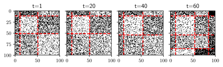
We first estimated $\hat{z}_{t}$ at each $t$ with $x_{t}$ using the variational Bayes method [30]. As there might be a so-called label switching problem (e.g., [31, 32]) for $\{\hat{z}_{t}\}_{t=1}$ , we applied ECR algorithm [33, 34] to reorder their blocks. We calculated the code-length for model $M$ as $L(M)=\log{2.865}+\log{M}+\log{\log{M}}+\dots$ in Eq. (III-B) [10], where the sum is taken for all the positive terms. We also calculated the code-length for models $M_{1}$ and $M_{2}$ as $L(M_{1},M_{2})=L(M_{1})+L(M_{2}|M_{1})$ . $L(M_{2}|M_{1})$ is code-length necessary for encoding $M_{2}$ given $M_{1}$ , that is,

\displaystyle L(M_{2}|M_{1})=\begin{cases}-\log{(1-\alpha)}&(M_{1}=M_{2}),\\ -\log{\alpha/(K-1)}&(M_{1}\neq M_{2}),\end{cases}

(25)

where $K$ denotes the maximum number of models, and $\alpha\mathrel{\overset{\makebox[0.0pt]{\mbox{\tiny def}}}{=}}(N_{t}+1/2)/(t+1)$ means the Krichevsky-Trofimov estimator [35]. Here, $N_{t}$ is the number of model changes until $t-1$ . We set $K=10$ and all the confidence parameters $\delta=\delta_{X|Z}=\delta_{Z}=0.05$ . We repeated the procedure for 20 times. Fig. 3 shows the estimated number of blocks and the MDL change statistics $\Phi_{t}$ , $\Phi^{Z}_{t}$ , and $\Phi^{X|Z}_{t}$ . We observe the following results from Fig. 3:

•

$\Phi_{t}$ changed at $t=20$ , $40$ and $60$ . This means that abrupt changes occurred at level 1, 2, and 3, respectively.
•

$\Phi^{Z}_{t}$ changed at $t=40$ and $60$ . This means that abrupt changes occurred at level 2 at $t=40$ and at level 3 at $t=60$ .
•

$\Phi^{X|Z}_{t}$ changed at $t=20$ and $60$ . This means that abrupt changes occurred at level 1 at $t=20$ and at level 3 at $t=60$ .

Fig. 3: MDL change statistics for 20 datasets with abrupt changes at

t=20

(level 1),

t=40

(level 2), and

t=60

(level 3): (a)

\Phi_{t}

, (b)

\Phi^{Z}_{t}

, and (c)

\Phi^{X|Z}_{t}

. Window size

h=2

VI-A2 Evaluation Metrics

For evaluation, we investigated the trade-off between the detection delay and accuracy for a change point $t^{\ast}$ in terms of the benefit and the false alarm rate of a detected change point $\hat{t}$ , which are defined as

	$\displaystyle\mathrm{benefit}$	$\displaystyle=\max\left(1-\frac{\|\hat{t}-t^{\ast}\|}{T},0\right)\quad(\hat{t}>t^{\ast}),$		(26)
	$\displaystyle\mathrm{FAR}$	$\displaystyle=\frac{\|\{t:t^{\ast}-U<t<t^{\ast},\phi_{t}>e\}\|}{\|\{t:t^{\ast}-U<t<t^{\ast}\}\|},$		(27)

where $(t^{\ast},\phi_{t},e)=(60,\Phi_{t},\epsilon)$ (level 3), $(t^{\ast},\phi_{t},e)=(40,\Phi_{t}^{Z},\epsilon_{Z})$ (level 2), and $(t^{\ast},\phi_{t},e)=(20,\Phi_{t}^{X|Z},\epsilon_{X|Z})$ (level 1). $U$ denotes the period for which overdetection is not allowed. In this experiment, We set $T=5$ and $U=10$ in Eq. (26) and (27), respectively.

VI-A3 Methods for Comparison

We evaluated the performance of HCDL by comparing it with benchmark methods. We used the following three methods as benchmarks:

•

The conventional MDL change statistics-based method (NML). We used the MDL change statistics-based change detection, which employs the NML code-length in Eq. (5) instead of Eq. (6). We abbreviate this method as NML. It can detect changes at level 3 only but can not decompose them in a hierachical way. Sakai and Yamanishi [36] proposed an efficient approximate formula for the generalized relation model including SBM, and we use it.

•

Tracking the Best Expert (TBE) [19]. Herbster and Warmuth developed the fixed share algorithm, abbreviated as FS. It was originally designed to make predictions by taking a weighted average over a number of experts. In FS, the expert with the largest weight is the best expert. We can think of FS as a model change detection algorithm by tracking the time-varying best expert. We updated each weight $w_{t,k}^{s}$ for expert $k$ at time $t$ as

$\displaystyle w_{t,k}^{m}$	$\displaystyle=w_{t,k}^{s}e^{-\eta\left\|\mathrm{DNML}(x_{t},z_{t};K_{t})-\mathrm{DNML}(x_{t},\hat{z}_{t};k)\right\|},$	(28)
$\displaystyle\mathrm{pool}$	$\displaystyle=\sum_{k=1}^{K}\alpha w_{t,i}^{m},$	(29)
$\displaystyle w_{t+1,k}^{s}$	$\displaystyle=(1-\alpha)w_{t,k}^{m}+\frac{1}{K-1}(\mathrm{pool}-\alpha w_{t,i}^{m}),$	(30)

where $K_{t}$ means the true number of blocks at $t$ . The ratio parameter $\alpha$ of TBE was fixed to $\alpha=0.2$ .

•

DeltaCon [37]. Koutra et al. proposed a graph similarity-based approach to detect change points in dynamic networks called DeltaCon. It calculates feature similarity of each consecutive snapshot pair of networks. We define the change score as $1-\mathrm{similarity}$ .

We determined the threshold parameters for benchmark methods. They were tuned to minimize the harmonic mean of the average benefit and $(1-$ the false alarm rate $)$ at $t=60$ , at which a level 3 change occurred. For each procedure, we selected $\epsilon_{{}_{\mathrm{NML}}}\in\{0.1,0.5,1,2,5\}$ for NML, $\epsilon_{{}_{\mathrm{TBE}}}\in\{0.2,0.5,0.8\}$ and for TBE, $\epsilon_{{}_{\mathrm{Delta}}}\in\{0.02,0.025,0.03,0.035,0.04,0.045,0.05\}$ for DeltaCon, respectively.

Table I lists the average benefits and false alarm rates for each algorithm and each task: model change detection (change in $K$ ) and parameter change detection (changes in $\theta$ and $\pi$ ). The experimental results demonstrated that our proposed HCDL algorithm was able to detect hierarchical changes and identify their levels, which could not be discriminated by the benchmark methods. Note that DeltaCon is competitive with HCDL except the benefit at $t=20$ , but it can not inherently identify change levels.

TABLE I: Average benefits and FARs for each level of change for abrupt changes.

	Level 3 ( $t=60$ )		Level 2 ( $t=40$ )		Level 1 ( $t=20$ )
	benefit	FAR	benefit	FAR	benefit	FAR
HCDL ( $h=1$ )	$\mathbf{1.00\pm 0.00}$	$\mathbf{0.00\pm 0.00}$	$\mathbf{1.00\pm 0.00}$	$\mathbf{0.00\pm 0.00}$	$0.97\pm 0.03$	$\mathbf{0.00\pm 0.00}$
HCDL ( $h=2$ )	$\mathbf{1.00\pm 0.00}$	$\mathbf{0.00\pm 0.00}$	$\mathbf{1.00\pm 0.00}$	$\mathbf{0.00\pm 0.00}$	$\mathbf{1.00\pm 0.00}$	$\mathbf{0.00\pm 0.00}$
HCDL ( $h=3$ )	$\mathbf{1.00\pm 0.00}$	$\mathbf{0.00\pm 0.00}$	$\mathbf{1.00\pm 0.00}$	$\mathbf{0.00\pm 0.00}$	$\mathbf{1.00\pm 0.00}$	$\mathbf{0.00\pm 0.00}$
NML ( $h=1$ )	$\mathbf{1.00\pm 0.00}$	$0.03\pm 0.02$	$0.61\pm 0.04$	$\mathbf{0.00\pm 0.00}$	$0.96\pm 0.02$	$\mathbf{0.00\pm 0.00}$
NML ( $h=2$ )	$\mathbf{1.00\pm 0.00}$	$0.04\pm 0.03$	$0.63\pm 0.07$	$0.03\pm 0.05$	$\mathbf{1.00\pm 0.00}$	$\mathbf{0.00\pm 0.00}$
NML ( $h=3$ )	$\mathbf{1.00\pm 0.00}$	$\mathbf{0.00\pm 0.00}$	$0.64\pm 0.08$	$0.03\pm 0.05$	$\mathbf{1.00\pm 0.00}$	$\mathbf{0.00\pm 0.00}$
TBE	$0.44\pm 0.37$	$\mathbf{0.00\pm 0.00}$	$0.00\pm 0.00$	$\mathbf{0.00\pm 0.00}$	$0.00\pm 0.00$	$\mathbf{0.00\pm 0.00}$
DeltaCon	$\mathbf{1.00\pm 0.00}$	$\mathbf{0.00\pm 0.00}$	$\mathbf{1.00\pm 0.00}$	$\mathbf{0.00\pm 0.00}$	$0.85\pm 0.37$	$\mathbf{0.00\pm 0.00}$

VI-B Synthetic Dataset 2 (Gradual Change)

We generated a dataset in which each level of change occurs gradually.

For $t=1,\dots,90$ , we generated links $x_{t}$ between nodes as follows:

\displaystyle x_{t}\sim\begin{cases}\mathrm{SBM}\,(x_{t};\pi^{1},\theta^{1},K=3)&(t=1),\\ \mathrm{LinkTrans}(x_{t}|z_{t-1};\pi^{1},\theta^{1},\beta)&(t=2,\dots,9),\\ \mathrm{SBM}\,(x_{t};\pi^{1},\theta^{1,2}(t),K=3)&(t=10,\dots,15),\\ \mathrm{LinkTrans}(x_{t}|z_{t-1};\pi^{1},\theta^{2},\beta)&(t=16,\dots,34),\\ \mathrm{SBM}\,(x_{t};\pi^{1,2}(t),\theta^{2},K=3)&(t=35,\dots,40),\\ \mathrm{LinkTrans}(x_{t}|z_{t-1};\pi^{2},\theta^{2},\beta)&(t=41,\dots,59),\\ \mathrm{SBM}\,(x_{t};\pi^{2,3}(t),\theta^{3},K=4)&(t=60,\dots,70),\\ \mathrm{LinkTrans}(x_{t}|z_{t-1};\pi^{3},\theta^{2},\beta)&(t=71,\dots,90),\end{cases}

where $\mathrm{SBM}$ and $\mathrm{LinkTrans}$ are the same as in the abrupt change case in Section VI-A. The link probability $\theta$ gradually changes between $t=10$ and $t=15$ . Then, the mixture probability $\pi$ gradually changes between $t=35$ and $t=40$ . Finally, the model changes from $K=3$ to $K=4$ at $t=60$ , and then the mixture probability of the newly generated blocks gradually increases from $t=60$ to $t=70$ . Fig. 4 shows a sample sequence of $x_{t}$ .

The hyperparameter of $\pi^{1}$ was set to $\alpha=1$ (the Dirichlet distribution), and those of $\theta^{1}$ were set to $a=b=1$ (the Beta distribution). We set $\pi^{2}=(\pi_{1}^{1},(\pi_{2}^{1}+\pi_{3}^{1})/2,(\pi_{2}^{1}+\pi_{3}^{1})/2)$ and $\pi^{3}=(\pi_{1}^{3},\pi_{2}^{3},\pi_{3}^{3},\pi_{4}^{3})=(\pi_{1}^{2},\pi_{2}^{2},3\pi_{3}^{2}/4,\pi_{3}^{2}/4)$ . It means that the largest group $k=3$ is split into two blocks with the ratio of $3$ to $1$ between $t=60$ and $t=70$ . $\theta^{2}$ $(k,\ell=1,\dots,4)$ was set as follows: $\theta^{2}_{k,\ell}=\theta^{1}_{k,\ell}+u$ $(0\leq\theta^{1}_{k,\ell}+u\leq 1)$ , $1-\epsilon$ $(\theta^{1}_{k,\ell}+u>1)$ , and $\epsilon$ $(\theta^{1}_{k,\ell}+u<0)$ . Here, $u$ was drawn from the uniform distribution whose range is between $-0.1$ and $0.1$ , and $\epsilon$ was set to $\epsilon=10^{-6}$ . $\theta^{3}$ $(k,\ell=1,\dots,4)$ was set as follows: $\theta^{3}_{k,\ell}=\theta^{2}_{k,\ell}$ $(1\leq k,\ell\leq 3)$ , $\theta^{3}_{k,4}\sim\mathrm{Beta}(a,b)$ $(1\leq k\leq 4)$ , and $\theta^{3}_{4,\ell}\sim\mathrm{Beta}(a,b)$ $(1\leq\ell\leq 3)$ .

From $t=10$ to $t=15$ , $\theta^{1,2}(t)$ is defined as $\theta^{1,2}(t)=\theta^{1}+(t-10)(\theta^{2}-\theta^{1})/5$ , which means that $\theta$ started to change at $t=10$ and finally reaches $\theta^{2}$ at $t=15$ . Likewise, from $t=35$ to $t=40$ , $\pi^{1,2}(t)$ was defined as $\pi^{1,2}(t)=(\pi^{1}_{1},\pi^{1}_{2}+(t-35)(\pi^{1}_{3}-\pi^{1}_{2})/10,\pi^{1}_{3}-(t-35)(\pi^{1}_{3}-\pi^{1}_{2})/10)$ , which means that the third component of $\pi$ gradually decreases. Finally, the model changes at $t=60$ from $K=3$ to $K=4$ . Then, the mixture probability $\pi$ gradually changes between $t=60$ and $70$ as $\pi^{2,3}(t)=(\pi^{2}_{1},\pi^{2}_{2},\pi^{2}_{3}-(t-60)\pi^{2}_{3}/40,(t-60)\pi^{2}_{3}/40)$ , which means that the third component of $\pi$ decreases gradually, and finally the ratio of the third and the newly fourth components reaches $3$ to $1$ .

We repeated the procedure for 20 times. We set the maximum number of models $K=10$ and all the confidence parameters $\delta=\delta_{X|Z}=\delta_{Z}=0.05$ . Fig. 5 shows the estimated number of blocks and the MDL change statistics $\Phi_{t}$ , $\Phi_{t}^{Z}$ , and $\Phi_{t}^{X|Z}$ . We observe the following results from Fig. 5:

•

$\Phi_{t}$ started to change gradually at $t=10$ , $35$ , and $60$ .
•

$\Phi_{t}^{X|Z}$ started to change gradually at $t=10$ and $60$ . This means that changes at level 1 were found.
•

$\Phi_{t}^{Z}$ started to change gradually at $t=35$ and $60$ . This means that changes at level 2 were found.

Fig. 5: MDL change statistics for 20 datasets with gradual changes from

t=10

15

(level 1), from

t=35

40

(level 2), and from

t=60

70

(level 3): (a)

\Phi_{t}

, (b)

\Phi_{t}^{Z}

, and (c)

\Phi_{t}^{X|Z}

. Window size

h=2

VI-B1 Evaluation Metrics

For evaluation, we investigated the trade-off between the benefits in Eq. (26) and false alarm rate in Eq. (27) for a change point $t^{\ast}$ . Here, $(t^{\ast},\phi_{t},e)=(60,\Phi_{t},\epsilon)$ (level 3), $(t^{\ast},\phi_{t},e)=(35,\Phi_{t}^{Z},\epsilon_{Z})$ (level 2), and $(t^{\ast},\phi_{t},e)=(10,\Phi_{t}^{X|Z},\epsilon_{X|Z})$ (level 1). We set $T=5$ and $U=10$ in Eq. (26) and (27), respectively.

VI-B2 Methods for Comparison

We evaluated the performance of HCDL by comparing it with NML, TBE, and DeltaCon as in the abrupt change case. We selected the threshold parameters for each method by tuning them among the same values as in the abrupt change case.

Table II lists the benefits and false alarm rates of each algorithm. This shows the effectiveness of HCDL for a dataset in which the models and parameters are changing gradually. Note that NML, TBE, and DeltaCon can not identify the levels of changes; hence, their alarms are mixed for different levels. We evaluated these alarms for each of the different levels. Here again, we observe that the HCDL algorithm detected hierarchical changes and identified their levels, which could not be discriminated by the benchmark methods.

TABLE II: Average benefits and FARs for each level of change for gradual changes.

	Level 3 ( $t=60-70$ )		Level 2 ( $t=35-40$ )		Level 1 ( $t=10-15$ )
	benefit	FAR	benefit	FAR	benefit	FAR
HCDL ( $h=1$ )	$0.97\pm 0.09$	$\mathbf{0.00\pm 0.00}$	$0.96\pm 0.02$	$\mathbf{0.00\pm 0.00}$	$0.95\pm 0.04$	$\mathbf{0.00\pm 0.00}$
HCDL ( $h=2$ )	$0.98\pm 0.08$	$\mathbf{0.00\pm 0.00}$	$0.97\pm 0.03$	$\mathbf{0.00\pm 0.00}$	$0.98\pm 0.05$	$\mathbf{0.00\pm 0.00}$
HCDL ( $h=3$ )	$\mathbf{1.00\pm 0.00}$	$\mathbf{0.00\pm 0.00}$	$\mathbf{0.97\pm 0.02}$	$\mathbf{0.00\pm 0.00}$	$\mathbf{1.00\pm 0.00}$	$\mathbf{0.00\pm 0.00}$
NML ( $h=1$ )	$0.89\pm 0.10$	$\mathbf{0.00\pm 0.00}$	$0.61\pm 0.04$	$\mathbf{0.00\pm 0.00}$	$0.69\pm 0.10$	$0.04\pm 0.05$
NML ( $h=2$ )	$0.90\pm 0.10$	$\mathbf{0.00\pm 0.00}$	$0.62\pm 0.06$	$\mathbf{0.00\pm 0.00}$	$0.70\pm 0.10$	$0.04\pm 0.05$
NML ( $h=3$ )	$0.91\pm 0.09$	$\mathbf{0.00\pm 0.00}$	$0.63\pm 0.07$	$0.01\pm 0.02$	$0.71\pm 0.10$	$0.06\pm 0.05$
TBE	$0.04\pm 0.10$	$\mathbf{0.00\pm 0.00}$	$0.00\pm 0.00$	$0.02\pm 0.09$	$0.00\pm 0.00$	$0.10\pm 0.30$
DeltaCon	$0.89\pm 0.31$	$\mathbf{0.00\pm 0.00}$	$0.15\pm 0.37$	$0.01\pm 0.02$	$0.64\pm 0.48$	$0.01\pm 0.03$

VI-C Population Movement Dataset

We demonstrate the effectiveness of HCDL on the population movement dataset ²² 2 https://www.e-stat.go.jp/en/stat-search/database?page=1&toukei=00200523&tstat=000000070001. This dataset is presented by Ministry of Internal Affairs and Communications, Statistics Bureau, Director-General for Policy Planning & Statistical Research and Training Institute, Japan. It records the amount of the population that moved from a prefecture to another prefecture per month from April 2005 to March 2014. The total numbers of time points and prefectures are 108 and 47, respectively. We conducted HCDL on the dataset. In this experiment, we assumed that each number of population movement in each month between prefectures was drawn from the Poisson distribution. We set the window size $h=3$ for HCDL.

Fig. 6 shows that HCDL detected the changes between $t=72$ and $t=76$ , that is, from March to August in 2011. During the period the MDL changes statistics $\Phi_{t}$ increased more than other years. These changes corresponded to the population movement caused by the Great East Japan Earthquake in March 2011, the Japanese government’s announcement that the radiological dosage levels greatly increased in many regions in Japan in May 2011, and the announcement of population movement during June–August 2011 by Japanese government. It is particularly noticeable that $\Phi_{t}^{Z}$ increased in May and June 2011. It is hard to extract such information with the rival algorithms, DeltaCon [37] and Eigenspace-based method [5], as shown in Fig. 6 (d) and (e), because these algorithms can not decompose the change scores into each layer.

Fig. 6: Estimated number of blocks and change scores for Population Movement dataset. (a) Estimated number of blocks. (b) MDL change statistics

\Phi_{t}

. (c)

\Phi^{Z}_{t}

. (d)

\Phi^{X|Z}_{t}

. (e) change scores of DeltaCon [37]. (f) change scores of Eigenspace-based method [5]. Dashed red line indicates a period between March and August, 2011.

We then investigated why the changes scores $\Phi_{t}$ were higher in 2011 than those in other years. Fig. 7 shows the estimated blocks of each prefecture for the Population Movement dataset between January and August in 2010, 2011, and 2012. Each color represents each group for all the prefectures. We observe from Fig. 7 that the estimated blocks were different in May 2011, from these in other months in the same year or other years. We inferred that this led to the rise of $\Phi_{t}^{Z}$ in May and June, 2011. This corresponded to a change at level 2.

We further investigated what change occurred at the population movement, that is, at level 1 during the period. Fig. 6 (d) shows that $\Phi^{X|Z}_{t}$ increased more than these during the same months in other years. Fig. 8 shows the heatmaps of the numbers of population move among 14 prefectures between March and June in 2010, 2011, and 2012. Note that the numbers of the population movement are truncated at 2000 to easily compare the result. We observe from Fig. 8 that more people moved in April and May 2011 than other years, from Miyagi prefecture and Fukushima prefecture to the other prefectures. These two prefectures were hardest hit by the disaster. This corresponded to the change at level 1.

In summary, we are able to interpret the events behind the changes in terms of severity levels in the HCDL framework.

VI-D Enron Dataset

We demonstrate the effectiveness of HCDL on a dynamic social network constructed from the Enron corpus [38] ³³ 3 http://www.cs.cmu.edu/~enron/, which consists of about 0.5 million email messages. In this experiment, we extracted e-mails among 151 employees from April 1999 to August 2002. We preprocessed the corpus and obtained a connection matrix for each week by assigning 1 if employee $i$ sent at least one email to $j$ during the week, and 0 otherwise. We made no distinction between emails sent “To” and “Cc.”

Fig. 9 lists the estimated change scores for the Enron dataset. The horizontal axis represents the week index, while the vertical axis represents the change scores $\Phi_{t}$ , $\Phi^{Z}_{t}$ , and $\Phi^{X|Z}_{t}$ . We set the window parameter $h=4$ . We observe from Fig. 9 that, from $t=80$ to $t=90$ , $\Phi^{Z}_{t}$ and $\Phi^{X|Z}_{t}$ showed local sharp peaks, while $\Phi_{t}$ was relatively mild. Actually, Mr. Jeffrey Skilling took over as CEO in February 2001. It shows that this event corresponded to changes at levels 1 and 2. Around $t=110$ to $150$ , all of $\Phi_{t}$ , $\Phi^{X|Z}_{t}$ and $\Phi^{Z}_{t}$ had sharp peaks at several points. Actually, at $t=135$ , Enron collapsed in December 2001, and a number of related events occurred around this time. It shows that this event corresponded to changes at level 3.

We see from Fig. 9 that before and after Enron collapsed at $t=135$ , the number of blocks rapidly changed. We could see the messages between employees changed dynamically. We also see from Fig. 10 that the number of blocks rapidly changed before and after Enron collapsed at $t=135$ .

We could see the number of messages or relation between employees changed dynamically and it affected the number of group estimated with HCDL and the structures of blocks. It owes to the decomposed nature of DNML.

Fig. 9: Estimated blocks and change scores of the Enron dataset. (a) Estimated number of blocks. (b) MDL change statistics

\Phi_{t}

. (c)

\Phi^{Z}_{t}

. (d)

\Phi^{X|Z}_{t}

. (e) change scores of DeltaCon [37].

In this way, we are able to interpret the events behind the changes in terms of severity levels in the HCDL framework.

VII Conclusion

This study established HCDL to detect hierarchical changes in latent variable models. HCDL aims at detecting and explaining those changes. The idea is to employ an information-theoretic framework for change detection in which the MDL change statistics is used as a measure of the degree of change, in combination with the DNML code-length. We presented a rationale for reliable alarms of changes on the theory for hypothesis testing. With synthetic and real datasets, we demonstrated that HCDL is highly effective.

Acknowledgement

This work was partially supported by JST KAKENHI 191400000190 and JST-AIP JPMJCR19U4.

References

[1] T. A. B. Snijders and K. Nowicki, “Estimation and prediction for stochastic blockmodels for graphs with latent block structure,” Journal of Classification, vol. 64, no. 4, pp. 583–639, 1997.
[2] D. M. Blei, A. Y. Ng, and M. I. Jordan, “Latent dirichlet allocation,” Journal of Machine Learning Research, vol. 3, no. 4–5, pp. 993–1022, 2003.
[3] D. V. Hinkley, “Inference about the change-point in a sequence of random variables,” Biometrika, vol. 27, no. 1, pp. 1–17, 1970.
[4] M. Basseville and I. V. Nikiforov, Detection of abrupt changes: Theory and application. Prentice Hall, 1993.
[5] T. Idé and H. Kashima, “Eigenspace-based anomaly detection in computer systems,” in Proceedings of the tenth ACM SIGKDD International Conference on Knowledge Discovery and Data Mining (KDD), 2004, pp. 440–449.
[6] S. Hirose, K. Yamanishi, T. Nakata, and R. Fujimaki, “Network anomaly detection based on eigen equation compression,” in Proceedings of the 15th ACM SIGKDD International Conference on Knowledge Discovery and Data Mining (KDD), 2009, pp. 1185–1194.
[7] L. Akoglu and C. Faloutsos, “Event detection in time series of mobile communication graphs,” in Proceedings of 27th Army Science Conference, 2010.
[8] T. Funke and T. Becker, “Stochastic block models: A comparison of variants and inference methods,” PLOS One, vol. 14, no. 4, p. e0215296, 2019.
[9] J. Rissanen, “Modeling by shortest data description,” Automatica, vol. 14, pp. 465–471, 1978.
[10] ——, Optimal estimation of parameters. Cambridge, 2012.
[11] K. Yamanishi and K. Miyaguchi, “Detecting gradual changes from data stream using MDL-change statistics,” in Proceedings of 2016 IEEE International Conference on Big Data (BigData), 2016, pp. 156–163.
[12] K. Yamanishi and S. Fukushima, “Model change detection with the MDL principle,” IEEE Transactions on information theory, vol. 9, no. 64, pp. 6115–6126, 2018.
[13] T. Wu, S. Sugawara, and K. Yamanishi, “Decomposed normalized maximum likelihood codelength criterion for selecting hierarchical latent variable models,” in Proceedings of the 23rd ACM SIGKDD International Conference on Knowledge Discovery and Data Mining (KDD), 2017, pp. 1165–1174.
[14] K. Yamanishi, T. Wu, S. Sugawara, and M. Okada, “The decomposed normalized maximum likelihood code-length criterion for selecting hierarchical latent variable models,” Data Mining and Knowledge Discovery, vol. 4, no. 33, pp. 1017–1058, 2019.
[15] B. Kim, K. Lee, L. Xue, and X. Niu, “A review of dynamic network models with latent variables,” Statistics surveys, vol. 12, pp. 105–135, 2018.
[16] L. Akoglu, H. Tong, and D. Koutra, “Graph based anomaly detection and description: A survey,” Data Mining and Knowledge Discovery, vol. 29, pp. 626–688, 2015.
[17] S. Ranshous, S. Shen, D. Koutra, S. Harenberg, C. Faloutsos, and N. F. Samatova, “Anomaly detection in dynamic networks: A survey,” WIREs computational statistics, vol. 7, no. 3, pp. 223–247, 2015.
[18] K. Yamanishi and Y. Maruyama, “Dynamic model selection with its applications to novelty detection,” IEEE Transactions on Information Theory, pp. 2180–2189, 2007.
[19] M. Herbster and M. Warmuth, “Tracking the best expert,” Machine Learning, no. 2, pp. 151–178, 1998.
[20] T. Erven, P. Grünwald, and S. D. Rooji, “Catching up faster by switching sooner: A predictive approach to adaptive estimation with an application to the AIC-BIC dilemma,” Journal of the Royal Statistical Society: Series B (Statistical Methodology), vol. 74, no. 3, pp. 361–417, 2012.
[21] M. Song and H. Wang, “Highly efficient incremental estimation of gaussian mixture models for online data stream clustering,” in Proceedings of the SPIE, vol. 5803, 2005, pp. 174–183.
[22] J. Sun, S. Papadimitriou, P. S. Yu, and C. Faloutsos, “Graphscope: Parameter-free mining of large time evolving graphs,” in Proceedings of the 13th ACM SIGKDD International Conference on Knowledge Discovery and Data Mining (KDD), 2007, pp. 687–696.
[23] G. Rossetti and R. Cazabet, “Community discovery in dynamic networks: A survey,” ACM Computing Surveys, vol. 51, no. 2, p. 35, 2018.
[24] J. Gama, I. Žliobaitė, A. Bifet, P. Mykola, and B. Abdelhamid, “A survey on concept drift adaptation,” ACM Computing Surveys, vol. 46, no. 4, 2014.
[25] D. T. J. Huang, Y. S. Koh, G. Dobbie, and R. Pears, “Detecting volatility shift in data streams,” pp. 863–868, 2014.
[26] S. Hirai and K. Yamanishi, “Detecting latent structure uncertainty with structural entropy,” in Proceedings of 2018 IEEE International Conference on Big Data (BigData), 2018.
[27] ——, “Detecting model changes and their early signals using MDL change statistics,” in Proceedings of 2019 IEEE International Conference on Big Data (BigData), 2019.
[28] Y. Ohsawa, “Graph-based entropy for detecting explanatory signs of changes in market,” The Review of Socionetwork Strategies, pp. 1–21, 2018.
[29] S. Fukushima and K. Yamanishi, “Detecting metachanges in data streams from a viewpoint of MDL,” Entropy, vol. 21, no. 12, p. 1134, 2019.
[30] M. Mariadassou, S. Robin, and C. Vacher, “Uncovering latent structure in valued graphs: A variational approach,” vol. 4, no. 2, pp. 715–742, 2010.
[31] R. Redner and H. Walker, “Mixture densities, maximum likelihood and the EM algorithm,” SIAM Review, vol. 26, pp. 195–239, 1984.
[32] A. Jasra, C. Holmes, and D. Stephens, “Markov chain monte carlo methods and the label switching problem in bayesian mixture modeling,” Statistical Science, vol. 20, pp. 50–67, 2005.
[33] C. Rodriguez and S. Walker, “Label switching in bayesian mixture models: Deterministic relabelling strategies,” Journal of Computational and Graphical Statistics, vol. 23, no. 1, pp. 25–45, 2014.
[34] P. Papastamoulis and G. Iliopoulos, “An artificial allocations based solution to the label switching problem in bayesian analysis of mixtures of distributions,” Journal of Computational and Graphical Statistics, vol. 19, pp. 313–331, 2010.
[35] R. E. Krichevsky and V. K. Trofimov, “The performance of universal encoding,” IEEE Transactions on Information Theory, vol. 27, no. 2, pp. 199–207, 1981.
[36] Y. Sakai and K. Yamanishi, “An NML-based model selection criterion for general relational data modeling,” in Proceedings of IEEE International Conference on Big Data (BigData), 2013, pp. 421–429.
[37] D. Koutra, N. Shah, J. T. Vogelstein, B. Gallagher, and C. Faloutsos, “DeltaCon: A principled massive-graph similarity function with attribution,” ACM Transactions on Knowledge Discovery from Data, vol. 10, no. 3, p. 28, 2016.
[38] C. E. Priebe, J. M. Conroy, D. J. Marchette, and Y. Park, “Scan statistics on enron graphs,” Computational and Mathematical Organization Thoery, vol. 11, no. 3, pp. 229–247, 2005.

Detecting Hierarchical Changes in Latent Variable Models

Abstract

Index Terms:

I Introduction

I-A Motivation

I-B Novelty and Significance

I-C Related Work

II Problem Setting

III Information Theoretic Methods for Change Detection

III-A MDL Change Statistics

Definition III.1.

III-B DNML Code-Length

Definition III.2.

Theorem III.1.

IV Theory for Making Reliable Alarms

IV-A Error Probabilities for Change Detection

Theorem IV.1.

IV-B Choosing Threshold Parameters

V Hierarchical Change Detection

VI Experiments

VI-A Synthetic Dataset 1 (Abrupt Change)

VI-A1 Dataset

VI-A2 Evaluation Metrics

VI-A3 Methods for Comparison

VI-B Synthetic Dataset 2 (Gradual Change)

VI-B1 Evaluation Metrics

VI-B2 Methods for Comparison

VI-C Population Movement Dataset

VI-D Enron Dataset

VII Conclusion

Acknowledgement

References

Detecting Hierarchical Changes
in Latent Variable Models