Pseudomodes for non-self-adjoint Dirac operators
Abstract.
Depending on the behaviour of the complex-valued electromagnetic potential in the neighbourhood of infinity, pseudomodes of one-dimensional Dirac operators corresponding to large pseudoeigenvalues are constructed. This is a first systematic approach which goes beyond the standard semi-classical setting. Furthermore, this approach results in substantial progress in achieving optimal conditions and conclusions as well as in covering a wide class of previously inaccessible potentials, including superexponential ones.
1. Introduction
1.1. Motivations
Spectral theory of self-adjoint operators has exhibited an enormous development since the discovery of quantum mechanics at the beginning of the last century and it can be regarded as well understood in many respects by now. Recent years have brought new motivations for considering non-self-adjoint operators, too, notably due to the unconventional concept of representing physical observables by operators which are merely similar to self-adjoint ones [3]. This brand-new construct, nicknamed quasi-self-adjoint quantum mechanics, remained overlooked for almost hundred years and has led to challenging mathematical problems which cannot be handled by standard tools and the theory is by far not complete.
It has been accepted by mathematicians as well as physicists that an appropriate characteristic which conveniently describes the pathological properties of non-self-adjoint operators is the notion of pseudospectra [29, 12, 18]. Given a positive number , the -pseudospectrum of any operator in a complex Hilbert space is defined as its spectrum enriched by those complex points (called pseudoeigenvalues) for which there exists a vector (called pseudoeigenvector or pseudomode or quasimode) such that
| (1.1) |
This notion is trivial for self-adjoint (or, more generally, normal) operators, because then merely coincides with the -tubular neighbourhood of the spectrum. If is non-normal, however, the pseudospectrum can contain points which lie outside (in fact, possibly “very far” from) the spectrum . It turns out that it is the pseudospectrum which determines the decay of the semigroup generated by as well as the behaviour of the spectrum of under small perturbations.
The usefulness of pseudospectra in quasi-self-adjoint quantum mechanics was pointed out by Siegl and one of the present authors in [27]. Based on the semiclassical construction of pseudomodes in Davies’ pioneering work [11] (see also [30] and [13]), we proved an abrupt lack of quasi-self-adjointness for the prominent imaginary cubic oscillator of [4], which stayed at the advent of the so-called -symmetric quantum mechanics. Many other Schrödinger operators with complex-valued potentials were included in the subsequent works [22, 19, 20, 25, 24, 21, 23, 2].
In this series of works, the paper [23] of Siegl and one of the present authors is exceptional in that it develops a direct construction of large-energy pseudomodes (i.e. those corresponding in (1.1) to with ), which does not require the passage through semiclassical Schrödinger operators. In fact, the semiclassical setting follows as a special consequence of [23]. Moreover, the newly developed, general approach of [23] enables one to cover previously inaccessible potentials such as the exponential and discontinuous ones. What is more, the technique is applicable to other models such as the damped wave equation [1].
The objective of the present paper is to extend the method developed in [23] to relativistic quantum mechanics by considering Dirac instead of Schrödinger operators. This extension is both mathematically challenging and physically interesting, because the Dirac equation is not scalar and the external electromagnetic perturbations are allowed to be fundamentally matrix-valued. We also remark that the present model is additionally relevant in the context of graphene materials. What is more, we substantially generalise the method of [23] on a technical level, which enables us to cover previously inaccessible potentials, including superexponential ones. Non-self-adjoint Dirac operators have attracted a lot of attention recently [8, 6, 7, 15, 9, 16, 5, 10], however, we are not aware of any result related to the construction of pseudomodes in -dependent WKB form.
1.2. The model and main results
Following the classical reference [28], we introduce the one-dimensional free Dirac operator by
with mass . We think of as an operator acting in the Hilbert space which is a direct sum of two spaces,
equipped with the inner product
| (1.2) |
Alternatively, we identify with or . It is well known that is self-adjoint if and one has
| (1.3) |
The free operator is perturbed by a complex matrix-valued potential . We write
where , and assume that , meaning that all the components with are complex-valued (scalar) functions belonging to . In the case of real-valued potentials, the special scenario and (respectively, and ) corresponds to purely electric (respectively, purely magnetic) fields. The special case and is known as the scalar potential. We keep the same terminology in the general, complex-valued case.
The perturbed operator is introduced as the maximal extension of the operator sum , where we denote by the same symbol the maximal operator of multiplication by the generated function . More specifically,
| (1.4) | ||||
The local integrability conditions imposed on the coefficients of ensure that all the actions of in (1.4) are well defined in the sense of distributions. By straightforward arguments, it follows that is a closed operator. However, the closedness of is inessential for our construction of pseudomodes. In fact, many of the constructed pseudomodes belong to , so the majority of our results apply also to any (possibly non-closed or trivial) extension of the sum initially defined on .
The main purpose of this work is to build a -dependent family such that
| (1.5) |
where is the norm associated with (1.2). The principal tool for this construction is the (J)WKB analysis (also known as the Liouville–Green approximation). In addition to investigating the rate of the decay in (1.5), we also address the question of describing the shape of the complex region depending on . The method used in Section 4 gives us a way to sketch the region which seems rather optimal, even for low regular potential. It is interesting to observe that the domain does not depend on the regularity of the potentials when the imaginary parts of and grow slowly at such as logarithmic one (see Example 4) or root-type with (see Example 5).
As a foretaste of our main theorems without going into technical details, we present here a very special example of (1.5) for real and purely electric perturbations. The following theorem is a particular consequence of Theorem 3.10 and Remark 3.12 below. From now on, and denote, respectively, the real part and the imaginary part of a function .
Theorem 1.1.
Let satisfy
| (1.6) |
and set and . Assume further that there exist continuous function
and, for all ,
Then, there exists a -dependent family such that
| (1.7) |
Although the matrix structure of the potential is rather simple, the assumptions of the above theorem allow us to touch a very large class of potentials. For example, the following functions for (the middle part of the functions for can be adjusted such that we have ) are covered:
- (1)
Polynomial-like functions with .
Here we choose . - (2)
Exponential functions with .
Here we choose . - (3)
Superexponential functions .
Here we choose .
Remark 1.2.
Condition (1.6) ensures that is “significantly non-normal”. Indeed, if is the formal adjoint of , i.e. , then it is straightforward to verify (at least algebraically) that the normality holds if and only if the following identities
hold simultaneously on . For matrix-valued potentials of more general structures, the asymptotics of the sum of the imaginary parts of the diagonal components and should be considered instead of the imaginary part of in (1.6), see condition (3.1) below.
1.3. Comparison between Schrödinger and Dirac pseudomodes
The Dirac setting is richer in that the perturbation is a matrix-valued function, while it is just a scalar potential in the Schrödinger case. Let us make a brief comparison of the present results with the Schrödinger situation considered in [23] (see Assumption I below in this article and [23, Ass. I]):
- (1)
Because of the unboundedness of the spectrum of both from below and from above, see (1.3), it is not surprising that we are able to construct pseudomodes for , while just the limit is relevant in the Schrödinger case.
- (2)
- (3)
- (4)
- (5)
Moreover, the class of functions whose derivatives are controlled by the functions is significantly extended in our assumptions. For example, the superexponential function of example 3 above does satisfy our assumption, while it is not covered by [23, Cond. (3.2)]. This more general result of the present paper is technically due to the freedom in the choice of the function above, while it is fixed to the canonical choice with some in [23].
1.4. Handy notations
Here we summarise some special notations which will appear regularly in the paper:
- (1)
, with a non-negative integer , is the set of integers starting from ;
- (2)
and ;
- (3)
and denotes respectively the power and the -th derivative of a function with ;
- (4)
We use the same symbol for -norms of both scalar- and vector-valued functions;
- (5)
For two real-valued functions and , we write (respectively, ) if there exists a constant , independent of and (or any other relevant parameter), such that (respectively, );
- (6)
if and ;
- (7)
for all ;
- (8)
for all .
1.5. Structure of the paper
The paper is organised as follows. In Section 2, we present a general scheme of constructing a pseudomode satisfying (1.5) for the Dirac operator by the WKB method. This scheme is applied to real ’s in Section 3, while more general complex curves are allowed in Section 4. Many illustrative examples are considered at the end of each of the two sections.
2. WKB construction
2.1. Warming-up
Let us start the scheme of constructing the pseudomode of the Dirac operator (1.4) satisfying (1.5) by searching it in the form
| (2.1) |
where depending on will be determined later. This structure of pseudomode allows us to pull out the off-diagonal terms of potential by the following step
By letting one of the two components of be zero, for example the second one, we can compute by :
Here we assume that on the support of the pseudomode; this will be ensured by the condition (2.10) later. In this way, we have relaxed the problem to finding such that
Here the differential expression is defined by
Remark 2.1.
In [1], in order to construct the pseudomode for a damped wave system, the authors transferred the problem into finding the pseudomode of a quadratic operator having the Schrödinger form. We, meanwhile, will establish the WKB construction directly for the Sturm–Liouville-like operator without converting it to the Schrödinger operator.
Let us consider a sufficiently regular and complex-valued function which will be determined later in the WKB process. We consider the formal conjugated operator
where
| (2.2) |
Let us denote
| (2.3) |
which will play the role of the remainder in the WKB analysis.
We consider in the form where is a cut-off function whose support is allowed to depend on ; it will be determined later in Section 3.2. Hence, the action of on can be expressed as
| (2.4) | ||||
The WKB strategy is as follows. For each , we look for the phase in the form
| (2.5) |
where functions are to be determined by solving ordinary differential equations (ODEs); the number will be chosen later depending on the maximal possible order derivative of . After that, we show that the exponential decay of allows the norm of the first two terms in (2.4) to decay exponentially according to (Proposition 3.9) and the norm of the final term to decrease with the rate power of (Theorem 3.10).
Starting with and putting into (2.3), we obtain
| (2.6) |
Here the second equality follows by solving the eikonal equation ; in this way, the second order of in is removed and the final order of has been reduced.
We can do the same trick for any . Replacing by in (2.3), we obtain
Here the functions with are naturally defined by grouping together the terms attached with the same order of , with the exception of which we include in the leading order term. In detail, the first functions are expressed by
and the last functions are
| (2.7) | ||||||
Requiring for all , we obtain ODEs which can be solved explicitly to find all by a recursion formula
| (2.8) | ||||
After solving these ODEs, the WKB remainder is
| (2.9) |
Remark 2.2.
Let us make some comments at this stage.
- (1)
The choice of the sign in the definition of will be determined by the sign of the sum at infinity and the sign of (see Remark 3.12).
- (2)
Since is a complex-valued function, the square root appearing in (2.8) is considered as the principal branch of the square root which is defined as, for ,
This principal branch of square root is holomorphic on . For that reason, the range of needs to stay away from such that the continuity (and/or the differentiability) of is deduced by the continuity (and/or the differentiability) of and . By writing (), this will be ensured if, by simple argument of product of two complex numbers,
(2.10) for all . If and are bounded, by considering very large, (2.10) is always satisfied. Otherwise, we need to employ the support of so as to make (2.10) happen.
Remark 2.3 (Beyond semiclassical).
It is a common knowledge that the limit of “large energies” in quantum mechanics is related to the “semiclassical limit”. While we indeed consider the spectral parameter in (1.5) diverging in the complex plane and employ WKB analysis standardly used for semiclassical regimes too (see, e.g., [14] for the Schrödinger operator or [17] for the magnetic Laplacian), there are some important novelties in our approach that we list here:
- (1)
Our spectral parameter not only plays the scaling role as semi-classical parameter , but also indicates the direction in which the large complex number will belong to the pseudospectrum.
- (2)
In the original WKB method applied to the spectral problems in the semi-classical regime, the solutions of the eikonal equation and the transports equations are independent of the semi-classical parameter. On the other hand, our solutions depend on the parameter and all estimates established for are necessary to be uniform in . This makes the present analysis considerably more demanding. However, both the WKB strategies share the same scheme that the eikonal solution plays a dominant part in deciding the decay of the main problem (the problem (1.5) in this case).
- (3)
While the semi-classical quasimodes always localise, the supports of our pseudomodes can be extended in some cases. Furthermore, the cut-off functions are occasionally needless in our WKB construction.
- (4)
While semi-classical works deal with smooth potentials, our framework can cover the potentials with low regularity (possibly discontinuous).
In summary, the present work goes beyond standard semiclassical settings. What is more, our approach is more robust in the sense that semiclassical results can be deduced as a consequence of it (cf. [23, Ex. 5.4]), but not vice versa (without the important developments mentioned above).
2.2. Structure of solutions of the transport equations and the WKB remainder
From now on, we assume that we are dealing with the plus sign in the formula of in (2.8), unless otherwise stated. Let us list some first solutions of the first transport equations to see which structure they are equipped with:
The remainder when we solve up to :
The remainder when we solve up to :
The remainder when we solve up to :
For , since the formulae of solutions are obtained from the recursion steps (2.8), if we want to write the formula of , the formulae of all with need to be explicitly given. It could be a challenging effort to find out the exact formulae for the transport solutions. However, the good news is that these solutions can be estimated without knowing their exact expression, instead a common structure of them is required. This is the content of the following lemma, but first, some notations should be introduced.
Notation 2.4.
Let be two functions which are assumed to be sufficiently regular so that all appearing derivatives of them exist. For , and , we employ the following notations
| (2.11) |
where
| (2.12) |
When , we make a convention that . Thus, if and for some , then .
Lemma 2.5.
For each , the maximal possible order derivative of in is and the maximal possible order derivative of and in is . Indeed, notice that, from the definition of and , the levels of the derivatives of and are equal to the levels of the derivatives of and while larger than the levels of the derivatives of and by one order. On the other hand, for all with and , we get
The remainders are controlled by the next lemma.
Lemma 2.6.
These lemmata can be proved, by induction, in the same manner as in Appendix of [23]. Therefore we omit the proofs here.
Remark 2.7.
At the end of this section, we want to show that choosing the shape of the pseudomode for the Dirac operator also plays important role technically. From the beginning, if we choose the basic form and insert it to the eigenvalue equation , we will have to deal WKB with the electromagnetic-like Schrödinger operator
Then its formal conjugated operator is described as follows
where
We see that this form of is very complicated to consider its square-root. Furthermore, by solving some firsts transport equations, we recognize that the sum attached with will destroy the structure of solutions of transport equations. These difficulties will make our WKB analysis unusable. Therefore, multiplying and with respectively, and not only gauges out and , but also allows this method to be workable.
3. Pseudomodes for
Let us recall here the picture of the Schrödinger operators to compare and outline the direction for the Dirac operators simultaneously. It is well known that the spectrum of the free Schrödinger operator (i.e. the Laplacian in with domain being the Sobolev space ) is given by the set . In [23], when the pseudoeigenvalue is real, the pseudomode of the Schrödinger operator with the complex-valued potential are constructed successfully when is positive and very large. Now, as mentioned in Section 1.2, the spectrum of the free Dirac operator is a set which is symmetric through the origin, see (1.3). Therefore, this evokes that the construction of the pseudomode for the Dirac operator for the positive and negative ’s can be established.
This expectation is also supported by looking at the structure of the WKB construction in both cases, especially the solution of eikonal equation which depends on the square root of :
Here, denotes the scalar potential in the Schrödinger operator. Assume that the real part of (respectively, real parts of and ) in the Schrödinger (respectively, Dirac) case is (respectively, are) bounded. Then the principal branch of the square root is well-defined only when in the Schrödinger case, while it is also able to be valid when in the Dirac case.
However, in this section, unless otherwise stated, we always assume that is positive. The case of negative can be considered analogously (see Remark 3.12 below).
3.1. General shapes of the potentials
Let us denote
Our main hypothesis reads as follows.
Assumption I.
Let , assume that , and there exist , by denoting , such that
- (1)
the sum of diagonal terms of has a different asymptotic behaviour at :
(3.1) and there exist such that
(3.2) - (2)
the primitive of the sum of off-diagonal terms is controlled by at : there exist such that
(3.3) - (3)
there exist continuous functions such that
(3.4) and, for all ,
(3.5) (3.6)
Notice that the first condition (3.1) implies that
| (3.7) |
Next lines gather some comments on Assumption I. Let us recall the expression of when :
| (3.8) |
We will see later that the shape of the pseudomode depends a lot on and the sign of (which is attached with very large ) will decide the sign for the decay of the pseudomode. The larger the sum is, the faster the pseudomode decreases at infinity (see the proof of Proposition 3.9). Furthermore, by looking at Remark 1.2, the assumption (3.1) also ensures that the operator defined in (1.4) is “significantly non-self-adjoint”.
From the conditions (3.2), we deduce the similarity of the sum of absolute values and the absolute value of the sum of and in the neighbourhood of infinity:
| (3.9) |
If , have the same signs at (or ), the condition (3.2) is obviously satisfied. Thus, these conditions guarantee that the opposite signs of and does not spoil the decay of the quasimode. As for the condition (3.3), it is easy to find and that can verify this. Indeed, since is positive at , the class of all functions and such that for all and for all will fulfil (3.3) completely.
3.2. Shapes of the cut-off functions
The role of the cut-off functions in the construction of pseudomodes is very important. Not all functions which are created from the WKB method would become the pseudomodes for the operator, since most of them do not belong to the domain of the operator. Therefore, the cut-off functions are added to complete this task. Furthermore, as discussed in Remark 2.2, when and are differentiable, in order to make the well-defined (i.e. non-multi-valued) and differentiable, the condition (2.10) need to be satisfied. It is obvious that (2.10) will be broken if or is not bounded. Thus, it is necessary to employ a suitable cut-off function whose support allows (2.10) to occur.
Let us denote by the cut-off function satisfying the following properties
| (3.10) |
where and are -dependent positive numbers which will be determined later. Notice that the cut-off can be selected in such a way that
| (3.11) |
To simplify the notation, we define the following sets
The next lemma is set up to define the boundary of the cut-off functions.
Lemma 3.1.
Let and let be a continuous function and let be a positive number, we define
| (3.12) |
Then can be infinite , however, when is unbounded at and for all sufficiently large , the number is finite and
| (3.13) |
Furthermore, if then
| (3.14) |
Proof.
When is unbounded at and , the number is finite. Given arbitrary , we consider , then , thus the unboundedness of is checked. In order to prove (3.14) under the assumption that , we assume opposite that there exists such that , then by the intermediate value theorem, there exists such that . This implies that which is a contradiction. ∎
By using Lemma 3.1, we introduce the boundary of the cut-off functions
| (3.15) |
through defining functions as follows
| (3.16) |
Here, , are fixed numbers such that and , in which will be chosen small enough later in Lemma 3.8.
Remark 3.2.
The continuity of will be given by the continuities of , (since they belong to ) and of . Note that, when is bounded at , i.e., all the functions and are bounded at , we have for all sufficiently large . In this case, we want to say that is constant on the positive side, i.e. for all . This remark is also the same for for the negative axis. In other words, sometimes we may not need the cut-off functions to localize the pseudomode.
When is finite, we define
| (3.17) |
Proposition 3.3.
There exists such that for all and for all , we have
- (1)
(3.18) - (2)
(3.19)
Proof.
In case , and are bounded at infinity, it is easy to check the above estimates. Now we assume that the unboundedness of or or at occurs. The case of unboundness at the negative infinity is analogous. It follows from the estimate (3.14) that, for all ,
Consequently, the three estimates in (3.18) follow. From them, we deduce that
Thus, The other direction is proved analogously, therefore the second estimate (3.19) is verified. ∎
3.3. Auxiliary steps
Lemma 3.4.
Proof.
We can choose satisfying for all , thanks to (3.13). Then, . From the formula of , the general Leibniz rule for the -th derivative of the product yields that
From the assumption (3.5), we obtain the estimate on ,
| (3.20) | ||||
where in the last step, we used (3.19) and the fact that (with some large ),
Next, we prove the estimate for . Let us recall that
The Leibniz rule also leads us to
Using Faà di Bruno’s formula for the derivative of a composition of two functions (see [26]), we get
where and are non-negative integers.
If , then and we have, on and for all ,
The last step is to the bound , and the fact that .
All the estimates for hold thanks to the boundedness of the appearing derivatives of on a compact set. ∎
We use the next lemma to gather all the real parts of the diagonal terms to one group and their imaginary parts to the other group. This allows us to estimate the denominator of in an easier way. Furthermore, it also tells us that the case is very special.
Lemma 3.5.
On , we have the following inequalities
| (3.22) | ||||
Proof.
Using the Cauchy–Schwarz inequality, we have
By an elementary inequality, the modulus of can be bounded from above as follows:
From this we can deduce successively that
∎
Lemma 3.6.
Proof.
Firstly, we prove the lemma for the first two estimates in (3.23). By looking at the formula of in (3.8) and using assumptions (3.1) and (3.2), we see that the numerator of has opposite signs at and . Namely, employing the remark (3.18) and recalling that , we have the following estimate on :
and similarly, on :
Next, it follows from the upper bound in (3.22) for the denominator of in (3.8) that, on ,
In the last step of the above expression, we used the estimates (3.18). On , we do it in the same manner.
Secondly, the final estimate in (3.23) is obtained by using the lower bound in (3.22) for the denominator of on :
Finally, let us prove the first estimate in (3.24) while the second one can be considered in a similar way. For , from Lemma 3.4, we have and Here we used the fact implied by (3.19) that, for all ,
| (3.25) |
Thus, applying this to control each element on :
in which we borrowed the definition of the set in (2.12). The estimate in (3.24) for follows from the formula of in Lemma 2.5. ∎
Remark 3.7.
From the estimates (3.23) and (3.9), it follows that, for all ,
The sign of the sum decides the sign of in the neighbourhood of infinity.
This is to be compared with the Schrödinger case [23, Lem. 3.4] where the sign of (with scalar now) plays this role, more precisely
In this case, when is considered to be large, needs to be proportional to (and larger than) near such that is also large. This was handled in [23] thanks to the definition of which is in terms of . Then needs to be controlled by such that can also be bounded by , whence the extra condition [23, Cond. (3.3)].
However, this extra work can been relaxed in the Dirac case thanks to the above form of . Technically, this can be explained by the product structure of which allows to show up in and therefore it cancels appearing in the denominator of asymptotically.
Furthermore, the case needs to be taken into account. For example, if this happens on (obviously, will be chosen in this situation), then the first estimate in (3.23) can be taken strictly as follows:
Meanwhile, the constant which turns up at (3.23), , is strictly smaller than and close to when is chosen small enough. However, it does not matter because this constant will be attached with as when we deal with it in the next lemma.
With the derivatives of given in (2.8), we can determine the primitives uniquely by choosing the initial data ,
Lemma 3.8.
Proof.
Let us recall that
From the formula of , we observe that
Then, it follows from the definition of the functions , and estimates in (3.19) that
Thanks to the estimate (3.23) and (3.24), , we have the uniform bound, for all ,
By the estimate (3.23) and (3.24) again, there exists a constant such that for all ,
To estimate the term with , we use the condition (3.3). Let be the number given in the condition (3.3). We choose very small such that
We deduce that, for all ,
To bound the terms with for , we apply (3.24) for all and obtain
| (3.26) |
Indeed, the case is bounded at is obvious. In contrast, we employ the property (3.14) of and the definition of function in (3.16), for all ,
and notice that for all . By employing (3.7), we have
| (3.27) |
Hence, the second inequality in the statement of this lemma is proved. The first inequality is obtained easily by the final estimate in (3.23), the observation (3.9) and the selected sign of the sum in (3.1) for all , Finally, combining this with (3.27), we obtain the result.
When , there is no presence of in and thus the integral will not come out in the above estimates, but the integral appears instead. However, if , we can perform the proof as we have done above. ∎
The next proposition reveals that the terms attached with the derivatives of the cut-off function decay exponentially as at a rate controlled by the function .
Proposition 3.9.
Let Assumption I hold for some . Let , be determined by (2.8) with the plus sign in the formula of and defined as in (2.5). Let be given in (3.10) whose , and is identified by (3.15), (3.16) and (3.17). Let us denote
| (3.28) |
Then as . More precisely, there exists such that, for all ,
where (with some )
and
Furthermore, if , the statement is also true for , i.e. is allowed.
Proof.
First of all, we want to show that the denominator in (3.28) is bounded from below by a constant not depending on . Thanks to Lemma 3.8 and the boundedness of for on , one has
Now, we try to control two terms attached with and in the numerator of (3.28). Obviously, the case of being bounded at is trivial, since on . The negative case is the same. We just need to care about the remaining situations in which is a “true” cut-off function. The main idea is to employ the exponential decay in order to limit the growth of polynomials on the support of and . In detail, applying Lemma 3.8 on the support of and (3.11), (3.17), we obtain (with some )
In the second inequality, we used the fact that increases as increases. Whereas the observation (3.7) is employed in the third inequality. The term associated with is estimated in the same way. Just notice that, from the similarity in (3.19), Lemma 3.4, Lemma 3.6 and estimates as in (3.26) for all , we have (with some )
Thus, the desired claim follows. ∎
3.4. Main results
Now, we can state our main theorems and their consequences.
The following theorem says that if at least belong to and at least belong to and satisfy Assumption I, our WKB solution will become the quasimode for the problem (1.5). When the potential is symmetric, the sufficient conditions for the involving spaces of are released to and of are released to in some cases. Furthermore, the rate of decay of the estimate when is symmetric is better in some situations.
Theorem 3.10.
Proof.
Before going to the proof, it is necessary to check that belongs to the domain of . With the choice of in the statement of the theorem, we have the relation between and as follows: Thus, if and only if
Obviously, this happens if is a “true” cut-off. The thing that makes us worry, for example, is the case when is bounded at . From the observation (3.7) combined with Lemma 3.8 and mimicking the proof of Proposition 3.9, it yields that, for sufficiently large (with some ),
From (2.4), we obtain
We will see later that is uniformly bounded from above. Therefore, the -integrability of is ensured by the -integrability of .
Theorem 3.11.
Proof.
Since , Lemma 3.8 and Proposition 3.9 still hold when . However, we can perform the estimates in Theorem 3.10 more strictly. Now, we assume that or is not bounded at . In detail, from the estimate of the remainder in (2.13) together with Lemma 3.4 and for , we obtain
For , for all , we have
While for all ,
In the second inequality, we employed (3.25). Notice that, if is unbounded, from (3.14) and the definition of in (3.16), we have for all and thus for all ,
in all cases of . From this, we obtain the estimates in the statement for all , even in the case and bounded at . The proof for is fulfilled in the same way. ∎
Remark 3.12.
Let us make some comments about the shape of the pseudomodes in connection with the sign of and the sign of :
- (1)
If and the sum of the diagonal terms of changes its sign in the assumption (3.1), i.e.
(3.29) then we just need to choose the minus sign in the formula of in (2.8). Then, we have
By repeating the procedure when proving (3.23), we have
(3.30) Therefore, the function
will play the same role as function . Although all the other terms also change their sign, it does not matter because they are all estimated with absolute value. Only the sign of is crucial. Thus, we still assume the same remaining hypotheses in Assumption I, but is replaced by and we have the same outcomes as stating in the above theorems.
- (2)
Let and Assumption I hold. What we need to do is to slightly change into in some places such as in Lemma 3.1. We redefine with being given in the same way as in (3.16). When is large enough, it follows, as in (3.18), that for all :
In this case, we will choose the minus sign in the formula of in (2.8) and we obtain the same results as in (3.30). Then, the method of the current section still works for the pseudomode construction and the outcomes of the above theorems are analogous.
In summary, from the two remarks above, our scheme suggests that the sign of the solution of the eikonal equation should be chosen as in the following table:
| on | on | |
| on | on | |
3.5. Applications
We consider some special examples of the matrix-valued potentials which satisfy Assumption I.
Example 1.
Let us list some smooth potentials defined on such that and Assumption I holds true. From that, we can apply Theorem 3.11.
- 1)
and are bounded at :
where is some smooth function on such that, with ,
Here we choose , for . Since are bounded both at and , the cut-off function is not needed for the pseudomodes construction. For all , there exists such that, for all ,
- 2)
is bounded but is unbounded at :
where is any smooth function on such that, with ,
Here we choose , for . Following (3.16) and (3.15), for large enough, the boundary of the cut-off can be computed approximately as and thus with some , It implies that, for all , there exists such that, for all , we have
- 3)
Example 2 (Polynomial-like diagonal terms).
Let us take a look at the potential satisfying Assumption I with , (for simplicity) and
with , for . It is necessary to assume that such that the sum of the imaginary parts of the diagonal terms satisfies the condition (3.1). Theorem 3.10 provides us with the fact that (i.e. we need and ) is enough to treat all kinds of potentials satisfying Assumption I. However, we would like to see what type of potential that can be treated and how fast the decay is when the potential is more regular. For that purposes, let us consider two cases in Theorem 3.11:
- Case 1:
and are bounded at . This happens if and only if . The application of Theorem 3.11 yields that, for all ,
Furthermore, in this case, the pseudomodes globally localise on without being attached with cut-off functions.
- Case 2:
or is not bounded at (i.e. ). We consider two smaller cases:
- i)
and and are bounded at . We do not use cut-off in this situation and for all ,
as . In the case , we employed (3.25).
- ii)
or or is unbounded at . Then, the possible maximum order of denoted by is , i.e. . Of course, and thus we can compute Applying Theorem 3.11 again, it results that, for all ,
as . We see that in the second case, can cover all the potentials such that For example, can treat
- (i)
, with .
- (ii)
, with and .
- (i)
- i)
The same thing happens as in the Schrödinger case: the pseudomode with is sufficient to treat all polynomial-like potential (even the case , see Theorem 3.10). The pseudomode associated with suffices for potentials growing not faster than linearly.
Example 3 (Exponential potentials).
Consider following potentials satisfying Assumption I. Since we would like to apply Theorem 3.11, we will assume further that for the sake of simplicity.
- 1)
- 2)
- 3)
- 4)
Superexponential functions:
In this example, we choose for . From (3.15) and (3.16), we can compute, with some constant , that
when large enough. Clearly, we have the following rough estimate
where is the number appearing in Proposition 3.9. Thus, we obtain and there exists a constant such that From Theorem 3.10, we have
4. Pseudomodes for large general pseudoeigenvalues
In this section, we want to construct the pseudomode corresponding to a complex pseudoeigenvalue
The interesting part is that the shape of the pseudospectral region is also revealed in the process of the construction. If the large real part of played a decisive role in the decaying estimation in the previous section, the imaginary part will take on this role in this section. We shall pay attention to the class of potentials whose and are identical, i.e. , and increasing on . The WKB analysis will be performed around a turning point which is defined by the equation
| (4.1) |
Since the non-zero part of the pseudomode will live completely in , it will be more convenient to consider the operators on , instead of . The application of the results for the class of operators on is easily obtained by the trivial extension of the pseudomode of the operators on .
4.1. Allowable shapes of the potentials
Since we do not have to bound the derivatives of components of on a fixed compact set as in Section 3, the whole space of them can be enlarged to , instead of . In order that the turning point is uniquely determined, we will assume that is strictly monotone for sufficiently large . The assumptions (3.5) and (3.6) are kept the same in this section, so that we can control the transport solutions. To be more specific, we make the following hypothesis.
Assumption II.
Let and , assume that and satisfy the subsequent conditions:
- (1)
the imaginary parts of and are equal, i.e. satisfy
(4.2) and there exist such that, for all ,
(4.3) (4.4) - (2)
the sum is controlled above by :
(4.5) - (3)
the derivatives of are controlled by , for ,
(4.6) and the differences between and (their derivatives) are controlled by polynomials
(4.7)
Comparing with Assumption I, although there are more conditions for the imaginary parts of the diagonal terms, the class of admissible potentials is still very large. Furthermore, our assumption allows to cover functions which grow slowly at such as logarithmic ones. This is interesting because the analogous hypothesis [23, Ass. 5.2] for Schrödinger operators does not allow for this kind of functions.
Remark 4.1.
We have the following helpful properties
- (1)
As discussed in [23, Sec. 3], when the condition (4.6) immediately implies that and are bounded. Thus the rising of in (4.2) needs to go along with the condition . Furthermore, when , we can deduce from the condition (4.4) that, for large enough and every ,
(4.8) In other word, the values of can be comparable up to a constant. The proof of (4.8) can be found in [23], but for the reader’s convenience, we recall the proof in a simpler way, for
In the last inequality, we used the observation that, for all and for ,
(4.9) The case is treated similarly.
- (2)
The cut-off in this case is constructed such that the pseudomode lives around the turning point . Namely, we arrange
| (4.11) | ||||
with
| (4.12) |
We see that if , the support of the pseudomode is able to be extended on when . As the WKB construction for the real pseudoeigenvalue, for each and each , the pseudomode has the form
| (4.13) |
where
4.2. Main results
Now, we can state our main theorem in the setting of this section.
Theorem 4.2.
Let Assumption II holds. Assume that there exists a (-dependent) such that the following conditions hold as , for all ,
| (4.14) | ||||
and
| (4.15) |
Let be determined by (2.8) and defined as in (4.13). We choose
- (1)
the plus sign in the formula of in (2.8) if ,
- (2)
the minus sign in the formula of in (2.8) if .
Then, for every , there exists such that, for all ,
in which
- •
- •
with .
The first condition in (4.14) is exactly the condition (2.10) that allows the regularity of pseudomodes be inherited from the regularity of the potential through the principal square root of . The last two conditions in (4.14) are inspired from the first ones in (3.18) for the real case of . In order to restrain the wild growth of , we require (4.15). Through the statement of the Theorem 4.2, it not only indicates the existence of the pseudomode, but also gives us a way to sketch the pseudospectrum around the infinity by looking for the admissible (see Subsection 4.5). The quantity always has an exponential decay at the rate control by the general function . This is also an improvement upon [23, Thm. 5.1] whose rate is only controlled by some polynomial.
4.3. Intermediate steps
On the way to prove our main results, some useful lemmata are designed similar to lemmata used in Subsection 3.3.
Lemma 4.3.
Let the assumptions of Theorem 4.2 hold. There exists such that, for all , for all and for all ,
Proof.
Lemma 4.4.
Proof.
By working as in (3.22), we also have the inequalities for dealing with the denominator of ,
| (4.16) | ||||
Notice that, there are two cases:
- (1)
If on , then the formula of has the expression
- (2)
If on , then the formula of has the expression
By using the second estimate in (4.16) and observing the sign of the term on the left and on the right of on , it implies that, for all ,
The rest upper bound for the integral of on is given by the first estimate in (4.16) and (4.14).
For all , by changing variable twice in integrals, we have
From (4.8), it yields that, for all ,
| (4.17) |
Using this approximation, we obtain the following lemma.
Lemma 4.5.
4.4. Proofs of the main results
Proof of Theorem 4.2.
Fix and consider defined in the statement of the theorem. We start the proof by showing that
| (4.20) |
By choosing in Lemma 4.5 sufficiently small such that , we can write for some . The plan is to use the upper bound of in Lemma 4.5 to control the terms in the numerator of (4.20) and employ the lower bound of for the denominator. We start with the term attached with :
In the second inequality, we used (4.15) and the fact that is increasing as goes far from . Furthermore, all appearing polynomial terms will be restrained, with some positive constants , by
| (4.21) | ||||
which follows directly from (4.17), the definition of in (4.12) and the condition (4.3) and (4.10). Thus, we have
| (4.22) | ||||
The second term in the numerator is bounded in the same manner. In detail, we look at the expression
For all and for all , thanks to (4.15) and (4.10), we have
The term related to is estimated as same as . Then, from (4.18), we have
Therefore, we also obtain the same estimate as (4.22) for the term attached with in (4.20). We consider in Lemma 4.5 such that , then it leads to
Using (4.17) and choosing small enough, we have
and similarly
Then, (4.20) follows by choosing sufficiently small and (4.21).
4.5. Applications
Let us list here some examples which are direct consequences of Theorem 4.2. We will see that the shape of the pseudospectrum depends not only on the type of the potentials, but also on their regularity.
Example 4.
First of all, we want to consider a kind of logarithmic potential on :
| (4.23) |
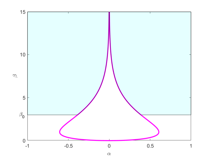
where , with , is such that as . Then all conditions of Assumption II are satisfied with and any . Given , then is determined by the relation About the quantity for , on account of the estimate (4.21), it decays in a superexponential way independent of the choice of , with some constant , . Since , the condition (4.14) of Theorem 4.2 are clearly satisfied if and only if
| (4.24) |
While (4.15) is assured if and only if
| (4.25) |
Therefore, we consider two cases:
From the definition of , we see that the pseudospectral region contains even points which stay very close to the line when and when large enough (see Figure 1).

Example 5.
Next, we want to study the polynomial-like potential on in the following form
| (4.28) |
where , with such that for . Then all the conditions of Assumption II are satisfied with and any . Given , then is determined, see (4.1), by From the estimate (4.21), for any , the quantity has an exponentially decay, with some ,
Since , the constraints in (4.14) imposed on are satisfied if and only if
| (4.29) |
We can compute directly the left-hand side of (4.15) as a function of : We consider two cases:
- (1)
If , we may take as (with )
Next, we are concerned about how small can be chosen such that we have the decay of . For large enough, we have
In order to have a decay for as , we choose
In summary, for any , there exist and a family such that
has the decay at the polynomial rate and the pseudospectral region is defined as
(4.30) - (2)
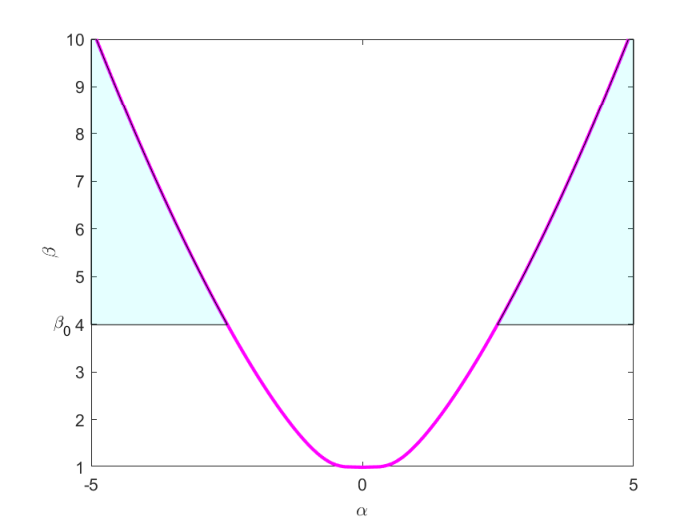
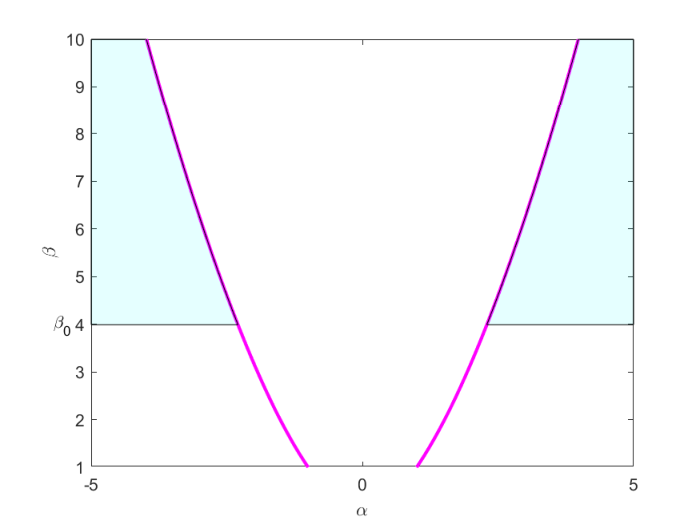
The reader is also invited to compare our results with the application of the same method for Schrödinger operators with the polynomial potential with in [23, Ex. 5.3]. We see that the pseudospectra of the Dirac operators are larger than those of the Schrödinger operators. While the outcome is kept between two curves in the Schrödinger case, the outcome in the Dirac case is just bounded from below by a curve. Technically, this can be explained by the appearance of in the denominator of the estimate for the Schrödinger operator, in which the above bound of is employed (to be clear, [23, Est. (5.9)]). Furthermore, [23, Ex. 5.3] only investigates the case , while ours produce the results for even . Finally, the decay of the problem in [23] is attained only when large enough, while our method gives us the decay even for small . In Figure 2, we see some representatives for the shape of corresponding to the power and the value of (when ). For the faster growing of the polynomial, the pseudospectrum region stands further away the axis .


Example 6.
The next example that we want to study is the potential whose is an exponential function:
| (4.34) |
where , , with , such that as . All conditions of Assumption II are satisfied with and any . Given , the turning point is determined by the relation For any , thanks to (4.21), there is some such that
Again, since the conditions in (4.14) are equivalent to the fact (4.29). We may take that is, with some , such that the condition (4.31) is satisfied. Under this choice of , we can bound above
In order to get the decay of as , we choose
In conclusion: for any , there exist and a family such that
where
| (4.35) |
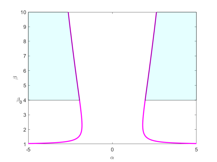
In Figure 3, some sketches are created for the the imagination of the pseudospectral region in the exponential cases. As in the polynomial cases, the higher is, the further stays away from the axis .
Acknowledgement
The authors were supported by the EXPRO grant number 20-17749X of the Czech Science Foundation (GAČR).
References
- [1] A. Arifoski and P. Siegl. Pseudospectra of the damped wave equation with unbounded damping. SIAM J. Math. Anal., 52(2):1343–1362, 2020.
- [2] V. Arnaiz. Construction of quasimodes for non-selfadjoint operators via propagation of Hagedorn wave-packets. arXiv:2010.14967 [math.AP].
- [3] F. Bagarello, J.-P. Gazeau, F. H. Szafraniec, and M. Znojil, editors. Non-selfadjoint operators in quantum physics: Mathematical aspects. Wiley-Interscience, 2015. 432 pages.
- [4] C. M. Bender and P. N. Boettcher. Real spectra in non-Hermitian Hamiltonians having symmetry. Phys. Rev. Lett., 80:5243–5246, 1998.
- [5] L. Cossetti, L. Fanelli, and D. Krejčiřík. Absence of eigenvalues of Dirac and Pauli Hamiltonians via the method of multipliers. Comm. Math. Phys., 379:633–691, 2020.
- [6] J.-C. Cuenin. Estimates on complex eigenvalues for Dirac operators on the half-line. Integral Equations Operator Theory, 79(3):377–388, 2014.
- [7] J.-C. Cuenin. Eigenvalue bounds for Dirac and fractional Schrödinger operators with complex potentials. J. Funct. Anal., 272:2987–3018, 2017.
- [8] J.-C. Cuenin, A. Laptev, and C. Tretter. Eigenvalue estimates for non-selfadjoint Dirac operators on the real line. Ann. Henri Poincaré, 15(4):707–736, 2014.
- [9] J.-C. Cuenin and P. Siegl. Eigenvalues of one-dimensional non-self-adjoint Dirac operators and applications. Lett. Math. Phys., 108(7):1757–1778, 2018.
- [10] P. D’Ancona, L. Fanelli, and N. M. Schiavone. Eigenvalue bounds for non-selfadjoint Dirac operators. Nonlinear Anal., 214:112565, 2022.
- [11] E. B. Davies. Semi-classical states for non-self-adjoint Schrödinger operators. Comm. Math. Phys., 200(1):35–41, 1999.
- [12] E. B. Davies. Linear operators and their spectra. Cambridge University Press, 2007.
- [13] N. Dencker, J. Sjöstrand, and M. Zworski. Pseudospectra of semiclassical (pseudo-) differential operators. Comm. Pure Appl. Math., 57(3):384–415, 2004.
- [14] M. Dimassi and J. Sjöstrand. Spectral Asymptotics in the Semi-Classical Limit. London Mathematical Society Lecture Note Series. Cambridge University Press, 1999.
- [15] A. Enblom. Resolvent estimates and bounds on eigenvalues for Dirac operators on the half-line. J. Phys. A: Math. Theor., 51:165203, 2018.
- [16] L. Fanelli and D. Krejčiřík. Location of eigenvalues of three-dimensional non-self-adjoint Dirac operators. Lett. Math. Phys., 109:1473–1485, 2019.
- [17] Y. Guedes Bonthonneau, T. Nguyen Duc, N. Raymond, and S. Vũ Ngọc. Magnetic WKB constructions on surfaces. Rev. Math. Phys., 33(7):Paper No. 2150022, 41, 2021.
- [18] B. Helffer. Spectral theory and its applications. Cambridge University Press, New York, 2013.
- [19] R. Henry. Spectral instability for the complex Airy operator and even non-selfadjoint anharmonic oscillators. J. Spectr. Theory, 4:349–364, 2014.
- [20] R. Henry. Spectral projections of the complex cubic oscillator. Ann. H. Poincaré, 15:2025–2043, 2014.
- [21] R. Henry and D. Krejčiřík. Pseudospectra of the Schrödinger operator with a discontinuous complex potential. J. Spectr. Theory, 7:659–697, 2017.
- [22] M. Hitrik, J. Sjöstrand, and J. Viola. Resolvent estimates for elliptic quadratic differential operators. Anal. PDE, 6:181–196, 2013.
- [23] D. Krejčiřík and P. Siegl. Pseudomodes for Schrödinger operators with complex potentials. J. Funct. Anal., 276(9):2856–2900, 2019.
- [24] D. Krejčiřík, P. Siegl, M. Tater, and J. Viola. Pseudospectra in non-Hermitian quantum mechanics. J. Math. Phys., 56(10):103513, 32, 2015.
- [25] R. Novák. On the pseudospectrum of the harmonic oscillator with imaginary cubic potential. Int. J. Theor. Phys., 54:4142–4153, 2015.
- [26] S. Roman. The formula of Faà di Bruno. Amer. Math. Monthly, 87(10):805–809, 1980.
- [27] P. Siegl and D. Krejčiřík. On the metric operator for the imaginary cubic oscillator. Phys. Rev. D, 86:121702(R), 2012.
- [28] B. Thaller. The Dirac equation. Texts and Monographs in Physics. Springer-Verlag, Berlin, 1992.
- [29] L. N. Trefethen and M. Embree. Spectra and pseudospectra. Princeton University Press, Princeton, NJ, 2005. The behavior of nonnormal matrices and operators.
- [30] M. Zworski. A remark on a paper of E. B. Davies. Proc. Amer. Math. Soc., 129:2955–2957, 2001.