Looking for obscured young star clusters in NCG 1313Journal: ApJFacilities: HST
Abstract
Using recently acquired HST NIR observations (J, Pa and H bands) of the nearby galaxy NGC1313, we investigate the timescales required by a young star cluster to emerge from its natal cloud. We search for extincted star clusters, potentially embedded in their natal cloud as either: 1. compact sources in regions with high H/Pa extinctions; 2. compact HII regions that appear as point-like sources in the Pa emission map. The NUV–optical–NIR photometry of the candidate clusters is used to derive their ages, masses and extinctions via a least SED broad and narrow–band fitting process. The 100 clusters in the final samples have masses in the range and moderate extinctions, mag. Focusing on the young clusters ( Myr) we derive a weak correlation between extinction and age of the clusters. Almost half of the clusters have low extinctions, mag, already at very young ages ( Myr), suggesting that dust is quickly removed from clusters. A stronger correlation is found between the morphology of the nebular emission (compact, partial or absent, both in H and Pa) and cluster age. Relative fractions of clusters associated with a specific nebular morphology is used to estimate the typical timescales for clearing the natal gas cloud, resulting between 3 and 5 Myr, Myr older than what estimated from NUV–optical–based cluster studies. This difference hints to a bias for optically–only based studies, which JWST will address in the coming years.
Keywords:
Young star clusters — Compact H II region — Star formation — Interstellar dust extinction — Spiral galaxiesI Introduction
Recent studies comparing the spatial distribution within galaxies of giant molecular clouds (GMCs) and HII regions suggest that GMCs spend most of their lifetime in an inert state. From the moment they begin to host star formation, their dense cores are quickly dissolved, on timescales of a few million years (Kobulnicky & Johnson 1999; Matthews et al. 2018; Kruijssen et al. 2019). Such short timescales, suggesting very efficient feedback from young stars, have been found with the same technique in various nearby galaxies and at different galactocentric distances (Kruijssen et al. 2019; Chevance et al. 2020a). According to these results, the star formation process is rapid and inefficient because feedback acts on very short timescales, resulting in only a small fraction of the gas being converted into stars (Matthews et al. 2018; Chevance et al. 2020b, e.g.).
Short feedback timescales have been typically derived in recent years by comparing tracers of different stages of the SF process. Corbelli et al. 2017 studied GMCs, embedded clusters (in the mid-infrared, MIR, where the extinction effect is lower) and exposed clusters (in H and UV bands) in the nearby galaxy M33, finding that young clusters remain in an embedded phase only for Myr on average. Similarly, Grasha et al. 2018; Grasha et al. 2019 found median ages of Myr for clusters associated to GMCs in NGC7793 and NGC5194. This also suggests that star clusters are able to emerge from their natal clouds long before the timescale required for clouds to disperse.
Star clusters play a fundamental role in the SF process, as most of the SF takes place in clustered environments (Lada & Lada 2003) and typically of the stars formed will evolve in bound systems (e.g. Bastian et al. 2012; Adamo et al. 2015; Chandar et al. 2015; Johnson et al. 2016; Messa et al. 2018a; Messa et al. 2018b and the review by Krumholz et al. 2019). Clustered star formation hosts most of the massive stars, responsible for the feedback regulating SF processes. The very early stages of cluster evolution can thus reveal, via the time needed to clear the gas and dust cloud around them, which feedback mechanism is mostly responsible for stopping star formation and therefore determining its efficiency. Whitmore et al. 2011 and Hollyhead et al. 2015 studied the morphologies of H emission associated to young clusters in the nearby galaxy M83, revealing that clusters are no longer embedded in their natal gas clouds by ages Myr, in agreement with the aforementioned studies of GMCs-clusters association. Hannon et al. 2019 measured a progression of the median ages when going from concentrated HII regions (median age Myr), to partially exposed ( Myr) to no H emission ( Myr). The same authors suggest that the typical timescale for gas clearing can be very short, on the order of Myr.
Almost all extragalactic young cluster studies are based on NUV-optical bands and therefore could be biased against extincted clusters (with extinctions higher than mag). Embedded clusters are likely extincted in the optical bands and can be revealed with longer wavelength emission. Radio observations can be used to directly detect the free-free emission from the gas ionized by newly formed massive stars (Kobulnicky & Johnson 1999; Johnson et al. 2001; Johnson et al. 2004; Johnson et al. 2009; Johnson & Kobulnicky 2003; Turner & Beck 2004; Aversa et al. 2011; Kepley et al. 2014, e.g.). The low detection rate of compact thermal radio sources is consistent with this embedded phase being short-lived (Tsai et al. 2009; Aversa et al. 2011, e.g.). Millimeter (and sub-millimeter) observations enable us to probe the molecular material in the vicinity of young star clusters (Finn et al. 2019; Johnson et al. 2015; Johnson et al. 2018, e.g.). Infrared emission can be used to trace the warm dust cocoons surrounding young clusters (Vacca et al. 2002; Johnson et al. 2004; Corbelli et al. 2017, e.g.), although the extent to which the infrared luminosities and colors can be used as diagnostics is highly dependent on the physical distribution of dust (Whelan et al. 2011, e.g.). Fully constraining the characteristics of embedded clusters requires this full wavelength coverage (from the radio to the infrared).
Typical mid-infrared (MIR) resolution ( for Spitzer) allows to resolve single clusters only for galaxies at close distances Mpc, making it difficult to build statistical samples. Already at a few Mpc, the SF clumps observable in the MIR bands may contain several star clusters (Lin et al. 2020, see e.g.). Studying MIR clumps on such scales ( pc) reveal sources with foreground extinctions up to mag (Elmegreen & Elmegreen 2019) and are useful to study the collapse of gas clouds (Elmegreen et al. 2018; Elmegreen & Elmegreen 2019; Elmegreen & Elmegreen 2020), but cannot trace the effect of feedback on the scale. The main unknown of the current studies on the gas clearing timescales is the possible effect of young embedded (and therefore possibly extincted) clusters, which are consistently neglected in studies of cluster populations focused on the optical-NUV bands (Whitmore et al. 2011; Hollyhead et al. 2015; Hannon et al. 2019, e.g.). With the present work we are filling this gap, by targeting the young and embedded clusters.
One way of combining high spatial resolution with the study of embedded star clusters is to rely on the infrared bands of HST. It is expected that newly formed clusters be surrounded by a dense compact (with radii of pc) cloud of gas and dust, that makes them extincted in the optical and NUV bands. Calzetti et al. 2015a already demonstrated how the use of near-infrared (NIR) HST band, and in particular the presence of NIR narrow-band filters, helps characterizing a highly extincted cluster (with foreground extinction mag and mixed attenuation from a cloud of mag in total), detected in the optical spectrum only in the I band, in the centre of NGC 5253.
In this work, we extend the NIR study of embedded clusters in the nearby galaxy NGC1313, a mildly-inclined () SBd galaxy at a distance of Mpc (Jacobs et al. 2009). Similarly to the study of Calzetti et al. 2015a we will use newly acquired HST-WFC3 NIR data, namely F110W, F128N and F160W, corresponding to J, Pa, and H bands. NGC1313 has a stellar mass of , an extinction–corrected (Calzetti et al. 2015b) and has been suggested to be currently in interaction with a satellite galaxy, that has produced a loop of HI gas around the galaxy (Peters et al. 1994) and a recent increase (on a timescale of 100 Myr) of the SFR in the south–west arm (Silva-Villa & Larsen 2012). Due to both its physical and morphological properties, with the presence of a bar and a rather irregular appearance, NGC 1313 has been compared to the Large Magellanic Cloud (de Vaucouleurs 1963). The star cluster population of NGC 1313 is quite numerous, with 673 clusters with ages Myr (Grasha et al. 2017a) of which 195 have compact morphology, ages Myr and masses (Ryon et al. 2017). The proximity of the galaxy, combined with the HST resolution allowed the study of its cluster population on physical scales pc and Ryon et al. 2017 finds a median cluster size of pc. Using HST narrow–band observations of NGC 1313 and of two galaxies at similar distance, Hannon et al. 2019 studied the morphology of H regions associated with the star clusters, estimating the typical timescales for a compact gas nebula to disperse ( Myr). We will, in the current work, complement the Hannon et al. 2019 study with our new NIR based analysis.
The paper is organized as follows: in Section II we present the HST observations used in this study, while in Section III we describe the methodology used to extract the catalogs of the young cluster candidates. In Section IV and V we present the analysis performed and the relative results. We discuss the results of our analysis in Section VI and summarize our findings in Section VII.
II Data
Recently acquired near infrared (NIR) photometry of NGC 1313 with the WFC3-IR camera, on board HST, covers two pointings of the galaxy with two broad-band (F110W and F160W) and one narrow-band (F128N) filters (GO program 15330; PI D. Calzetti). The narrow-band filter, centered at 1.283 , covers the wavelengths of the Paschen– (Pa) hydrogen recombination line emission. For each filter individual exposures were corrected for bias, dark and flat-field using the standard pipeline CALWF3 version 3.4.2. Images were aligned to the Gaia DR2 (Gaia Collaboration et al. 2018) reference frame using TweakReg, and mosaicked together using AstroDrizzle to a pixel scale of 0.08 arcsec/pixel. Proper motions were not applied in the alignment, as the high uncertainties of proper motions of extragalactic sources in the DR2 catalog would yield worse alignments, and poor subsampling in the mosaics. In this study we take advantage of the broad archival HST wavelength coverage of NGC 1313; in detail we use observations in five filters from the Legacy ExtraGalactic UV Survey (Calzetti et al. 2015b, LEGUS,) covering the NUV-optical range with broad-band filters (F275W, F336W, F435W, F555W and F814W) and in two additional filters from the LEGUS–H follow-up survey (GO-13773; PI R. Chandar) observing the galaxy with a narrow filter covering the H emission-line (F657N) and a medium-band filter sampling the line-free continuum (F547M). In total we have 10 filters spanning the wavelength range NUV-NIR, including two filters for the observation of the two hydrogen recombination lines H and Pa; details of the observations are summarized in Tab. 1. Fig. 1 (top left) shows a RGB–composite with H, F555W and Pa in the blue, green and red channels, respectively. We study the cluster population in the area delimited by the field of view of the NIR pointings, outlined in the same figure.
| Instrument | Filter | [Å] | Expt [s] | Program/PI |
|---|---|---|---|---|
| WFC3-IR | F160W | 15369 | 3594 | GO 15330/Calzetti |
| WFC3-IR | F128W | 12832 | 3594 | GO 15330/Calzetti |
| WFC3-IR | F110W | 11534 | 1994 | GO 15330/Calzetti |
| ACS-WFC | F814W | 8047 | 4569 | GO 9796/Miller |
| WFC3-UVIS | F657N | 6567 | 3090 | GO 13773/Chandar |
| WFC3-UVIS | F547M | 5447 | 1108 | GO 13773/Chandar |
| ACS-WFC | F555W | 5360 | 5600 | GO 9796/Miller |
| ACS-WFC | F435W | 4329 | 4560 | GO 9796/Miller |
| WFC3-UVIS | F336W | 3355 | 4818 | GO 13364/Calzetti |
| WFC3-UVIS | F275W | 2707 | 5058 | GO 13364/Calzetti |
III Source catalogs
We look for young dust-embedded star clusters following two separate approaches: (1) we define regions of high extinction, by constructing an extinction map from the combination of H and Pa emission line maps and looking for NIR compact sources within such regions; (2) we select, within the entire galaxy, sources with compact Pa line emission. In addition to the aforementioned source selections, we also consider the cluster catalog produced by LEGUS Adamo et al. 2017, based on HST observation in 5 NUV–optical broadband filters.
III.1 Sources in high-extinction regions
We make use of the observations in the UVIS-F657N and IR-F128N filters to construct H and Pa nebular emission-line maps. In order to estimate the continuum emission at the central wavelength of the F657N filter, we use two nearby filters, F547M and F814W. The former is a medium–band filter not containing nebular lines, the latter instead does contain emission lines, but its large bandwidth causes the flux to be greatly dominated, even for very young sources, by the stellar continuum; the nebular lines play only a minimal contribution. We linearly interpolate the observed flux on logarithmic scale in those two filters on a pixel–by–pixel basis, and we find, for every pixel of the data, the continuum corresponding to the pivot wavelength of the F657N filter, Å. This approach is made possible by the comparable widths of the PSF in the various HST optical filters, ensuring that the contribution to the flux in every pixel is coming from the same region in every observed band. Having subtracted the continuum, we are left with the combined emission of the H line and the [] doublet ( Å). In order to remove the contribution of the [] lines from the emission, we use their relative ratio to the H line as given by Kennicutt et al. 2008 (for NGC 1313, ).
We create a map of the Pa emission in a similar way, using F110W and F160W as nearby filters. We interpolate the flux in those two filters to estimate the value of the stellar continuum at the pivot wavelength of the F128N filter, Å. We point out that the F110W filter contains the Pa emission and therefore we use the first estimate of the Pa line emission map to create a line–free F110W map and then repeat the interpolation process. The second estimate of Pa emission line map differs from the first one by at maximum. Further iterations of this “cleaning” process differ from the previous ones by less than and quickly converge.
We convert the H and Pa emission maps to a common physical resolution by degrading the pixel scale of the H map from to arcsec/pix and then convolve each map to a gaussian kernel with px ( pc at the distance of NGC 1313), in order to smooth possible pixel–scale inaccuracies of the maps. We calculate the ratio H/Pa, correcting for the Galactic reddening:
| (1) |
where, for the Milky Way extinction law, (according to the parametrization of Fitzpatrick 1999, with total-to-selective extinction value ) and we used mag11 1 value taken from the NASA Extragalactic Database (NED). for the foreground extinction correction in the direction of NGC 1313. Finally, we convert the line ratio into an expected extinction value. Taking the intrinsic line ratio 22 2 appropriate for regions with electron temperature K, we assume that the different ratios observed over the different sub-regions of the galaxies are due to variations in the nebular extinction:
| (2) |
with . In constructing the extinction map we limit our selection to regions where both H and Pa line emissions have a S/N.
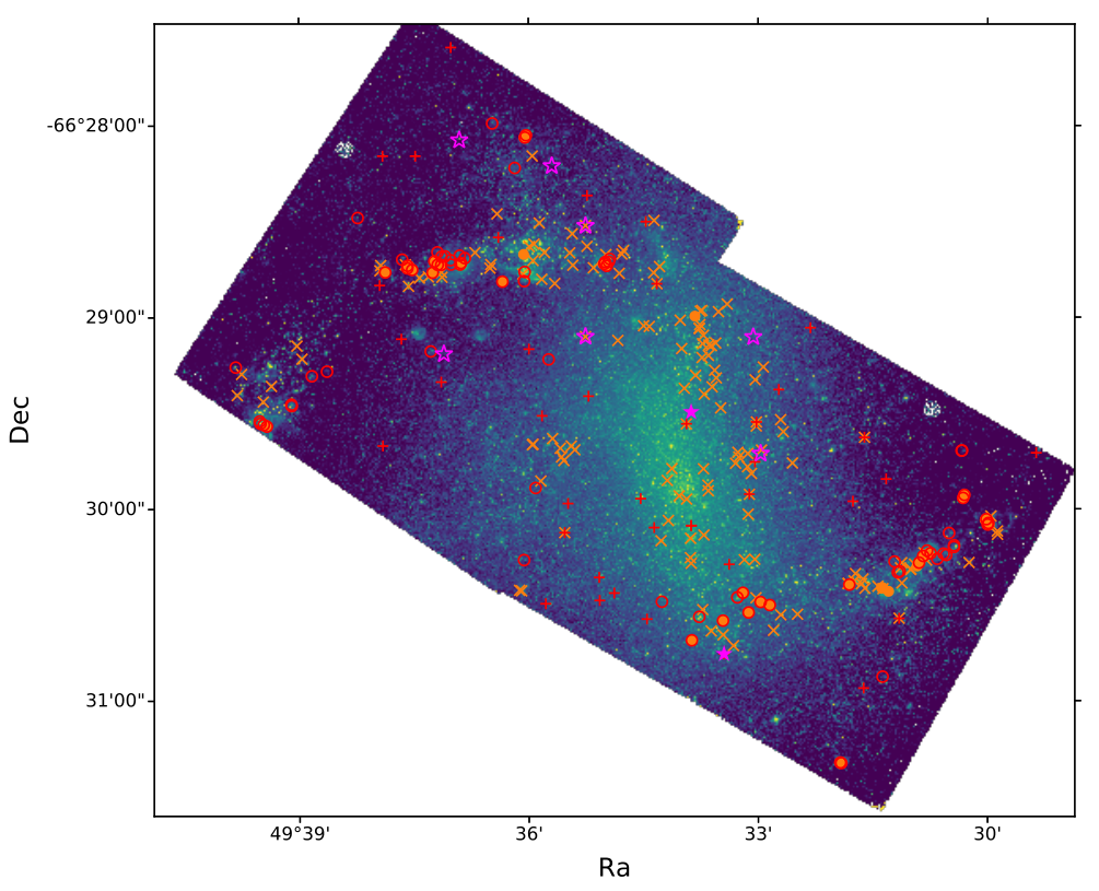
We show the extinction map in Fig. 1. In the same figure, as well as in Fig. 2, we compare it to the emission from the Spitzer telescope, revealing the dust emission. We find good spatial coincidence of the extincted nebular regions with the regions of brightest emission in . As expected, the extinction map reveals the extended regions along the spiral arms of NGC 1313 associated to recent star formation. In addition, it reveals compact regions with elevated values, associated with single sources; these latter cases are frequently caused by sources with high Pa emission but almost no H, mostly located along the spiral arms but with some exceptions.
Previous studies of clusters in NGC 1313 in the NUV-optical found on average extinctions of () for young clusters. We aim at studying clusters with higher extinction that may be missed in the NUV-optical bands. We therefore focus on the regions of the extinction map with mag and we visually select all the NIR sources with a clear counterpart in the F814W filter. We find a total of 188 cluster candidates. In the rest of the paper we are referring to this source catalog selected on the basis of the extinction map as ExtmapCat. We plot the positions of the sources within the galaxy in Fig. 1 (top right panel).


III.2 Sources with compact Paschen- emission
In order to search for sources not detected in H but emitting in Pa, and therefore missed by the extinction map (limited by the H detection), we select a second catalogue of sources. From the continuum–subtracted Pa map described previously, we select sources with detectable (S/N) Pa compact emission (i.e. with a narrow light profile, consistent with the one of stars and clusters, avoiding diffuse emission). This approach helps to detect embedded sources that have Pa detection but may be missed in H; this catalog and ExtmapCat are complementary, as they can overlap but are not mutually exclusive.
We retrieve 124 sources with compact Pa emission and for the rest of the paper we refer to this catalog as PBcompactCat. Of these, 40 are in common with the ExtmapCat. We plot the coordinates of the sources in this second catalogue in Fig. 1 (top left panel). While many sources reside in the extended regions of recent star formation outlined previously, some Pa-compact sources reside outside the main spiral arms.
In the same Fig. 1, we compare the position of sources in our catalogs with the position of MIR compact regions, selected in Spitzer observations by Lin et al. 2020. We remind that observations have a much lower resolution than the HST one, and that sources in the Lin et al. 2020 catalog were selected to have some HST cluster counterpart. Overall, the different catalogs cover similar regions of the galaxy; however, some of the Lin et al. 2020 sources are not present in our catalogs. In Fig. 2 we compare the spatial position of the nebular emission and emission with CO clouds found by ALMA (details on the data and of their analysis will be presented in a forthcoming paper, Finn et al., in prep.) focusing on three sub-regions of the galaxy. Also CO emission (which traces the GMCs) has a good spatial coincidence with emission and regions of elevated nebular extinction, with some visible exceptions; in the SW portion of the spiral arms, some CO clouds are displaced from the peak of nebular emission, suggesting the presence of gas which is still dark in NIR. The S region is instead mostly missed by the extinction map, or presents only low extinction values, mag, despite the presence of both CO and emission. A possible cause is that the entire S region is in a very early phase of star-formation, still invisible even in the NIR bands. This multi–band comparison shows how, while the sources extracted in ExtmapCat and PBcompactCat are distributed across the entire galaxy, some regions of early star formation may still be so obscured to be inaccessible in the HST NIR bands.
We point out that sources in both ExtmapCat and PBcompactCat were included in the catalogs without a detailed morphological classification; the two catalogs may therefore contain interlopers, such as bright stars. Photometry and size analyses are performed on all the sources (in Section IV), and their results will be used in Section V.1 and Section V.2 to clean the samples, producing final catalogs.

III.3 LEGUS catalogue
In the course of the current paper we will discuss our results in light of the results achieved by the study of the cluster catalog of NGC 1313 obtained by the LEGUS project. Such catalog was used to study the hierarchical distribution of young clusters (Grasha et al. 2017b; Grasha et al. 2017a), the distribution of their sizes (Ryon et al. 2017) and the typical evolution timescale associated to their HII regions (Hannon et al. 2019).
The methodology used to extract cluster catalogs in LEGUS is fully described in Adamo et al. 2017 and we direct the interested reader to that work for the details. We report here only few main points, relevant for the current work. The LEGUS cluster catalog of NGC 1313 was build upon 5 broadband filters, covering and bands. The optical data are the same used by this current analysis. In addition we used the data in the filters F675N and F546M already presented in Hannon et al. 2019. Ages and masses were derived via SED fitting of the 5 mentioned optical broad-bands only for cluster candidates brighter than mag in the band and with photometric detections in at least 4 of the bands. A visual morphological classification was used to separate centrally concentrated clusters from multi-peaked compact associations and to separate out contaminating sources (foreground stars, background galaxies, etc…) picked up by the initial source extraction. The spatial distribution of the clusters from the LEGUS catalog within the galaxy is shown in Fig. 1 (bottom right panel).
IV Analysis
At variance with the standard LEGUS SED analysis, we use in this work the information produced by the combined 10 bands photometry from NUV to NIR (Section IV.1) to estimate estimate ages, extinctions and masses of the sources in our catalogs (Section IV.3). We also use Pa and H equivalent width measurements as an independent way to estimate cluster ages (Section IV.4).
IV.1 Photometry
For all the catalogs we use a standard aperture photometry approach, using circular apertures with radii of 0.16’’ (4 px in the optical filters, 2 px in the NIR ones) in all bands. The sky background is estimated in an annulus centered on the source with radii of 0.20’’ and 0.28’’ by taking a clipped33 3 The clipping avoid considering pixels more than above the mean of the pixel values in the annulus. This helps eliminating sources from the background estimate. median. The value of the sky is then normalized by the area in the circular aperture and subtracted from the flux. Previous to the photometry, each source is centered using a centroid algorithm in the F814W filter and its coordinates are then kept fixed in all the other bands. We used F814W as reference because it is the reddest optical filter in our set. The NIR filters have an instrumental PSF which is roughly twice as large (in arcsec) compared to the one of the optical filters. Optical filters are therefore fundamental to discriminate multiple sources, i.e. separated by less than a few pixels transverse to the line of sight.
An aperture of 0.16” in radius includes of the flux for PSF-like light profiles, and this fraction decreases for wider light profiles. We apply an aperture correction to account for this missing flux. We consider as total flux the one enclosed in a circular aperture with a radius of 0.8’’. In order to estimate the aperture correction, we convolve the instrumental PSF44 4 Obtained from isolated stars in the data. of each filter with a Moffat profile (Elson et al. 1987), considered the most accurate function to describe the light profile of clusters (Elson et al. 1987; Bastian et al. 2013, e.g.). We take as reference value for the aperture correction the one obtained from a Moffat profile with an effective radius pc, as the distribution of cluster sizes is peaked at that value (Ryon et al. 2015; Ryon et al. 2017). Different choices of the aperture correction would change the normalization of the fluxes, but not the shape of the SED. In the context of broadband SED fitting they would have an effect only on the recovered masses, leaving unchanged ages and extinctions. We discuss different choices of aperture corrections in Section VI.1.
The radius of the photometric aperture was chosen as a compromise between including most of the sources’ fluxes within the aperture and avoiding contamination from nearby sources. Nevertheless, some of the sources suffer from contamination from the light of nearby sources. We consider as contaminated the cases where, within an aperture, the flux of nearby sources contributes at least of the total. 61 sources (out of 188, i.e. ) of the ExtmapCat have contamination in at least 1 filter, while for the PBcompactCat catalog the same is true for 16 sources (out of 124, i.e. ). Most of the contamination takes place in the bluer bands of our filter set, especially in the F275W and F336W filters. The source selection, focused on the red-optical and NIR filters can be a possible cause; many sources of the catalogs are bright in the red filters but their flux in the blue part of the spectrum appear dim, and therefore more easily contaminated by nearby sources.
IV.2 Cluster sizes and alternative photometry
The size of stellar clusters in NGC 1313 was studied in details in Ryon et al. 2017. The authors showed that the concentration index, CI (defined as the magnitude difference in circular apertures of 1 px and 3 px radii), is able to reproduce the overall distribution of sizes derived by more detailed means such as the software GALFIT. The advantage of using a such a simple metric is that it does not require any supervision, and therefore produces reliable results quickly. One possible limitation of the size estimates given by the CI is the presence of crowding, where nearby sources can greatly affect the measure of the CI.
In order to overcome this problem we implement an alternative measure of the sizes by performing a 2D fitting of the source. This method builds upon the size-photometry script described in Messa et al. 2019; we model the source with the stellar-PSF convolved with a Moffat profile, normalized by the flux and summed to a –degree polynomial that models the sky background. From each source we produce a cutout of the F814W data with px size that we fit, comparing it to the source model via a Levenberg-Marquardt minimization. This method was tested to be ineffective in discriminating sizes smaller than px (corresponding to pc at the distance of NGC 1313). We therefore consider all sources with px as consistent with having a stellar–PSF.
We use the size-photometry method just described also to perform a complementary photometry. In this case we do not rely on an (average) aperture correction, and the results are used to provide an estimate of the total flux of the clusters based on their sizes. For each source we keep fixed the central coordinates and the size retrieved in the F814W filter and then we repeat the Levenberg-Marquardt minimization in all the other filters, leaving only the flux (and the parameters describing the background) as free parameters. More details on this method are given in Appendix A. The photometric results obtained in this way are used in Section VI.1 to discuss the mass distribution of the cluster catalogs.
The comparison between the photometry obtained with this method and the one obtained via the aperture photometry analysis described in Section IV.1 is shown in Fig. 3. There is a magnitude offset of mag, especially clear for the ExtmapCat sources. This offset is caused by the aperture photometry method having a fixed aperture correction (calibrated on a typical cluster size, see previous section) as opposed to the size–photometry method. The right panel of Fig. 3 shows how the offset decreases when increasing estimated source sizes, being null at pc. Combining the information from the two panels in Fig. 3 we notice that the offset is mostly caused by bright sources with narrow profiles; these are probably stars and are excluded from the final samples (see Section V.1 and Section V.2). The same sources drive the narrow scatter of the distribution for the ExtmapCat compared to the PBcompactCat. Finally, the large overall scatter of the magnitude difference between the two methods (going from to mag) can be simply explained by the different sizes of the sources considered. When focusing on the sources at a fixed estimated size, the scatter reduces considerably (Fig. 3, central panel).
IV.3 SED fitting
We perform a least– fitting of the broadband SED obtained from the photometry in Section IV.1, following a very similar approach to the one used in LEGUS (see Adamo et al. 2017). We use as spectral models the Yggdrasil single-stellar population (SSP) models55 5 Available at https://www.astro.uu.se/~ez/yggdrasil/yggdrasil.html (Zackrisson et al. 2011). In details, we use the modes created from Starburst99 Padova-AGB tracks (Leitherer et al. 1999; Vázquez & Leitherer 2005) with a universal Kroupa 2001 initial mass function (IMF) in the interval . These models assume that the IMF is fully sampled. The stellar models are then used as input to run Cloudy (Ferland et al. 2013) and obtain the evolution of the nebular continuum and lines emission, produced by the ionized gas surrounding the young clusters. Yggdrasil adopts a spherical gas distribution around the emitting source, with hydrogen number density and gas filling factor (describing the porosity of the gas) , typical of HII regions (Kewley & Dopita 2002), and assumes that the gas and the stars form from material of the same metallicity. We consider a sub-solar metallicity () for NGC 1313 as it results in a best fit of the young clusters but we test also models with solar () metallicity (see discussion in Section V.1.1 and the figures in Appendix C.1). We choose the models with a gas covering fraction , i.e. only of the Lyman continuum photons produced by the central source ionize the gas. While Yggdrasil provides multiple choices for , we decide to keep it fixed, as it reasonably describe the case of ionized and partially leaking nebulae around young star clusters. Including the nebular emission in the cluster models is fundamental, and its omitting would lead to misleading results (Zackrisson et al. 2001; Reines et al. 2010; Adamo et al. 2010). Nevertheless, we do not have enough information to disentangle the gas conditions from our fitting process. We tested fitting the sources using models with i.e. no leakage of LyC photons, finding no substantial difference in the distribution of recovered cluster ages, masses and extinctions. We therefore kept models with as the reference one in our analysis.
Starting from the Yggdrasil models, we create a grid for the fitting by combining the spectra at progressive age steps and increasing internal reddening. We keep the same age steps included in Yggdrasil, which provides a interval frequency in the range . The sampling decreases at older ages but we are not affected by it, being interested in the very young sources. The models are reddened prior to being fitted using a foreground dust geometry with a grid of extinctions in the range with a step of mag. This is the only difference to the LEGUS approach, which used a grid of extinction extending only up to mag. We use as reference the Milky Way extinction law (Cardelli et al. 1989) but, as a test of the robustness of the results from our fit, we also consider the differential (i.e. the gas emission suffers higher extinction than the stars) starburst attenuation law (Calzetti et al. 2000). The fitting is done using a traditional approach on the grid just described. The model spectrum is normalized for each age-extinction combination in order to minimize the reduced (), for every source. The best fit for a source is given by the combination of age-extinction that minimize the value. An uncertainty interval is given for the best-fit parameters by considering all the sources within from the best-fit values, i.e. the parameters that result in a within 3.53 from the minimum .
Some of the sources in our catalogs have large photometric errors, while some others are contaminated, in some filters, by the emission of nearby sources, as described in Section IV.1. We decide to exclude from the fit the cases where the photometric uncertainty is above 0.3 mag (i.e. ), as sources with an uncertainty above that level have only a partial detection. We also exclude from the fit the cases of contamination, as their photometry would lead to misleading results. We fit the sources where at least 5 bands are left after the uncertainty-contamination cut, for a total of 170 sources for the ExtmapCat and 98 sources in the case of the PBcompactCat. The results of the fitting process are shown and described in Section V.
IV.4 H and Pa equivalent width analysis
A direct way of deriving the age of a cluster is to use the equivalent widths, EWs, of the nebular emission lines, defined as:
| (3) |
where is the observed flux across the emission line at the wavelength , and is the continuum level underneath the emission line. We do not have spectra of our sources and we have therefore to rely on a combination of broad and narrow filters to estimate the . Similarly to what done in Section III.1, we use the filters adjacent to the narrow one containing the line to estimate the continuum. For we use a logarithmic interpolation of the fluxes in the F547M and F814W filters to find the flux of the continuum emission at the pivotal wavelength of the F657N filter, . We calculate the flux in the H line by subtracting to the total flux measured in F657N, . From Eq. 3 we derive in our case:
| (4) |
where Åis the width of the narrow band filter.
In a similar way (using Åas the width of the narrow Pa filter), we derived EW(Pa) using F110M and F160W to estimate the continuum and consequently to measure the Pa line emission at , after using the iterative procedure for the F110W described in Section III.1.
We use the SSP models described in the previous section to estimate the EW expected at different cluster ages. The EW values that we measure depend on our specific set of filters, and therefore we cannot rely on theoretical values; we prefer instead to use directly the models to create a comparison set for the data. Fig. 4 shows the evolution of the H and Pa equivalent widths with age of the clusters for different metallicities and extinctions. From the definition in Eq. 3, the EW should not be affected by extinction, if lines and continuum are extincted in the same way. However, since we have to rely on a combination of broad and narrow filters, we see the measured EW being slightly different (typically ) at very young ages ( Myr) for different extinction values. Differential Starburst extinction is the one with the largest impact, acting more severely on the lines, (Calzetti et al. 2000) as can be appreciated from Fig. 4.
IV.5 Completeness test
We study the completeness of our samples, both in terms of photometry and of SED fitting. We built a control sample of sources with preset ages and masses, adding them to the observational data and going through the entire process of photometric analysis and SED fitting to recover their properties. We fix the sizes of the sources at px and the masses at ; these values, according to the results of our analysis presented in the next section (in particular Fig. 13 and Fig. 14) are reasonable assumptions. We simulate 100 sources for each combination of ages in the age range [1;6] Myr with steps of 1 Myr and of extinctions in the range [0;2] mag with steps of 0.25 mag, for a total of 30 combinations (3000 simulated sources). The galaxy is divided in grids of size and the simulated sources are located only in cells where at least one source from ExtmapCat or PBcompactCat is found. In this way we measure completeness in the same regions where the real data are located. Only 100 sources per time are inserted in the data–frames, in order to avoid biasing the photometry due to overcrowding.
We perform aperture photometry on the entire sample of simulated clusters; the almost totality of them have photometric uncertainties below 0.3 mag () for all ages and extinctions, in both F814W and F128N, the two filters used as the reference ones for the source extraction (the exact number is collected in Tab. 6 in Appendix B). We deduce that we are complete in the detection of the catalog up to a level between and . Most of the simulated sources have photometric uncertainties below 0.3 mag in at least 5 filters and are therefore fitted. Fig. 22 in Appendix B gives the exact number of such sources, at each age and extinction; their fraction stays around for sources up to extinctions of mag. For higher extinctions it decreases and strongly depends on the age.
We discuss in Section VI.2.1 the accuracy we have on the simulated clusters in retrieving the input ages and extinctions.
V Results
V.1 Ages, extinctions and masses of ExtmapCat
We show in Fig. 5 the best-fit age values of the sources in the ExtmapCat, along with their H and Pa EW values; we color code the sources according to their size, separating the ones with a light profile consistent with the instrumental PSF ( pc in the F814W filter), and therefore possibly stars, from those with larger size ( pc). Overall we find a good consistency between the ages derived from the SED fit and what could be expected from the EW values. We do not find sources with Myr with high EW in either H or Pa, confirming the general robustness of our fitting procedure. The largest differences of the EW values from the ones predicted (in Section IV.4) are at the youngest ages of 1 Myr, possibly caused by an inaccuracy in the derived ages. Confirming this hypothesis, we show in Appendix B how ages in the range Myr are degenerate. If, instead of the Milky Way extinction curve, we assume the differential starburst one, predictions and observation remain consistent with each other (see Fig. 5).
In Fig. 6 we show the same best-fit ages along with extinctions (left panels) and masses (right panels), and their uncertainties. We notice that the sources cover, unevenly, the entire age range considered in the model grids. We however point out that almost all of the sources falling in the last age bin considered (age Gyr) have a PSF-like light profile, consistent with being stars. Their masses are on average very high () but this is caused by considering them as very old and mildly extincted clusters. Most of the sources with best age between Myr and Gyr have large uncertainties, covering hundreds of Myrs. Many of the sources are aggregated around Myr of age and elevated extinction values; this can be due to degeneracies in the models causing artificial high extinction estimates for dim clusters (due to e.g. the presence of red supergiant stars), as discussed in Hannon et al. 2019.
In order to clean the catalog from sources with un-constrained properties, we leave out the sources with age uncertainties . In this way all the sources with an age uncertainty covering almost the entire range from to Myr are discarded (see the comparison between top and bottom panels in Fig. 6). We also leave out of the final sample most of the stellar-like sources; among the sources with pc, we keep only those with H and Pa equivalent width consistent with having ages Myr (i.e. with values of Åand Åin the case of H and Pa, respectively). We show the remaining sources in Fig. 6 (bottom panels). This final selection (ExtmapCat–final), counts 46 sources as reported in Tab. 2.
The recovered masses are mostly distributed in the range (Fig. 6, right panels). Sources with masses below can be expected to have an uneven sampling of the stellar initial mass function (IMF). This could cause the absence of massive stars able to ionize the gas surrounding the cluster, and, as consequence, the absence of line emission in our photometry. From a visual inspection of the broadband SEDs of our sample, we find that only 5 sources in the entire ExtmapCat sample are consistent with having a SED typical of very young (age ) clusters but show no or little line emission in H and Pa66 6 Despite the lack of compact line emission, such sources have been selected in the ExtmapCat sample because are located in regions of diffuse nebular emission.. The low number of clusters suffering from the lack of ionizing stars, despite the low range of masses recovered, could suggest an underestimation of the masses, due to a poor choice of the average aperture correction values. We discuss this possibility in Section VI.1.
We show the position of ExtmapCat–final sources within the galaxy in Fig. 7. They are all located in regions of recent star formation, mainly along the arms of the galaxy. Conversely, the sources discarded from the final selection are more scattered along the entire galaxy, confirming the reliability of our criteria in selecting young clusters.
Only 3 young sources with extinctions mag remain after the selections. We show the distribution of their from the fitting analysis, along with the broad–band SED in Appendix C.2 (Fig. 25). Two of them (C93 and C142) have high values for the best–fits , (). C10 is the best candidate for being young and highly extincted, with mag.
V.1.1 Testing metallicities and extinction laws
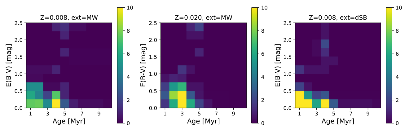
We performed the SED fit varying some of the model parameters, namely the metallicity and the extinction law. In order to better display the distribution of the sources in the age-extinction plane, along with their uncertainties, we use a density plot, based on a fixed grid of ages and extinction intervals (Fig 8). Each source is considered to cover all cells in the grid included within its upper and lower limits (both in age and E(B-V) values) as given by the face value the uncertainty. Its value in such cells is normalized by the number of the cells covered; in this way the final sum of the cell values over the entire grid is equal to the total number of sources considered. We use a grid with a 1 Myr step in ages in the range and a with a step of mag in the range .
We consider SSP models with solar metallicity for the fit and select a final sample in the same way as described in the previous chapter. The final sample counts the exact same sources as of ExtmapCat–final. We compare the recovered ages and extinctions using the density plot in Fig. 8 (central panel). On average, solar metallicity models recover slightly older and more extincted sources. The median recovered with the solar metallicity models is higher than the one of the reference sample (Fig. 9, left panel). An inspection of individual sources’ SEDs confirms that sub-solar models provide better fit to the photometry; photometric data containing strong emission lines show an abrupt increase of the flux in the filter F555W compared to F547M, despite their pivot wavelength being very similar. This difference is caused by different bandwidths, allowing F555W to include strong emission lines such as , in contrast to F547M. Different metallicities for the stellar models imply different strengths for the nebular lines and therefore different predicted fluxes, as shown for some examples in Fig. 24 in Appendix C.1. We conclude that the availability of both F555W and F547M filters allows us to disentangle the model-metallicity that gives a better agreement with the data, in this case sub–solar, 77 7 No observable difference was observed if a metallicity was considered..
We repeat all the analyses, included the final selection, using sub–solar metallicity models but implementing a differential starburst attenuation. The final sample selected remains almost identical to the reference ExtmapCat–final. The most notable difference is the presence of 2 additional sources as young-extincted cluster candidates, C33 and C175, whose distributions and best–fit fluxes are collected in Fig. 25. The distribution of ages and extinctions shown in the density distribution plots in Fig.8 reveals little difference from the reference case. On average, starburst extinction models recover younger and less extincted sources. The median recovered in this case is slightly larger than in the reference case (Fig. 9, right panel).

V.2 Ages, extinctions and masses of PBcompactCat
We show in Fig. 10 the best-fit age values for the sources in the PBcompactCat, along with the EW of H and Pa, comparing them to the EW from the models, again color–coding them according to their light-profile (red for stellar–like, green for larger). As in the previous sample, we find good consistency between the ages derived from the SED fit and H and Pa EW values. We note that there are no sources with , because of sample selection criteria. For the same reason, most of the sources with PSF–like light profiles have large H and Pa equivalent widths.
We show in Fig. 11 the best-fit values of ages, extinctions and masses, along with their uncertainties. The great majority of sources cluster around ages smaller than 10 Myr; we attribute this to the selection method of the sample, based on the observation of compact nebular emission and therefore biased towards young sources. We implemented the same selection criteria used for cleaning the ExtmapCat, reaching a final sample (PBcompactCat–final) counting 84 sources, 30 of which are in common with ExtmapCat–final (Tab. 2). These make most of the ExtmapCat, with some of the excluded sources being the young sources without line emission described in the previous section. We deduce that PBcompactCat–final is a more complete version of ExtmapCat–final. The distribution of PBcompactCat across the galaxy is shown in Fig. 7.
We analyze individually all the sources with mag in Fig. 26. For some of them, the best–fit reaches a high value, above 50 (C203, C228, C233, C240, C274) suggesting inaccurate fit results. For two of the sources (C239 and C251), the photometry from F657N filter was not used in the fit due to high uncertainty; nevertheless its value suggest no H emission, in contrast with the NIR filters suggesting Pa emission. Only three young–and–extincted sources, namely C213 (also included in the ExtmapCat–final sample under the ID number C10), C236 and C307, are good candidates for being retained in our final cut.
| ExtmapCat | PBcompactCat | |
| total | 190 | 124 |
| stellar | 136 (72%) | 39 (31%) |
| resolved | 54 (28%) | 85 (69%) |
| ExtmapCat–final | PBcompactCat–final | |
| total | 46 | 84 |
| stellar | 5 (11%) | 13 (15%) |
| resolved | 41 (89%) | 71 (85%) |
| in common | 30 | |
We show the resulting ages and extinctions from models with solar metallicity and with differential starburst extinction in Fig. 12 (top panels). The overall trends discussed in Section V.1.1 are recovered also in the PBcompactCat–final catalog, namely solar metallicity models predict older ages, while differential starburst extinction predicts younger ages and lower values. The reference models remain the most viable also in this case, with the lowest median values (Fig. 12, bottom panels).
V.3 Sizes
The distributions of cluster sizes, derived in Section IV.2, are showed in Fig. 13. The distributions have a median at pc in the case of ExtmapCat–final and pc in the case of PBcompactCat–final.
We can compare our results with those obtained by the study of LEGUS clusters sizes in NGC 1313 (Ryon et al. 2017), that found a median effective radius of pc with a dispersion pc. There are four major differences between our analysis and that of Ryon et al. 2017. First, the fitting method used is different (LEGUS used the software GALFIT, Peng et al. 2002; Peng et al. 2010). Second, the LEGUS analysis was limited to a sample of clusters with masses above and younger than Myr. Only 9 sources from our final catalogs reside in that range, while most of our sources have lower masses. Third, we use the F814W filter as the reference for fitting the size, while LEGUS used F555W. Finally, the analysis of (Ryon et al. 2017) is based on the LEGUS catalog and therefore ignores sources with stellar–like PSF (see also Adamo et al. 2017); for a better comparison we can re-estimate our median values excluding unresolved sources, finding pc and pc for ExtmapCat–final and PBcompactCat–final, respectively. While the difference in filters should not affect the resulting median sizes (assuming that the size is the same when observed in different bands), the difference in the age–mass range considered makes almost impossible a detailed comparison between the two results. Despite those differences, our values are consistent with Ryon et al. 2017 results within their uncertainties.
VI Discussion
VI.1 Mass estimates
We performed aperture photometry implementing an average aperture correction that assumes all clusters to be well–described by Moffat light profiles with pc. While the assumption is justified by studies of cluster sizes in NGC 1313 (Ryon et al. 2017), we discuss here whether using the individual size of each cluster in the photometric aperture correction would produce different mass estimates. We recall that different aperture corrections lead to different normalizations of the photometry, and therefore affect only mass estimates, leaving the recovered ages and extinctions unchanged.
The procedure for deriving photometric results considering the individual sources’ sizes was described in Section IV.2. We show in Fig. 14 the distributions of masses for ExtmapCat–final and PBcompactCat–final derived with the two photometric analysis. The mass distribution derived via the aperture photometry analysis is peaked at a slightly larger median value, for both catalogs. This is consistent with having found median effective radii of 1.28 and 1.18 pc for the ExtmapCat–final and PBcompactCat–final samples, respectively, smaller than pc used as reference for the average aperture correction. However, we note that the overall distributions are very similar, and we conclude that the mass distribution is not strongly affected by our choice of the average aperture correction.
We compare the median masses from our sample to the ones of the NGC1313 LEGUS cluster sample. For this comparison, we select from the LEGUS catalogs only sources with ages Myr (the range covered by our final samples), and with visual class 1, 2 or 3, hence avoiding class 4 (that according to the LEGUS classification contains non–clusters, see Adamo et al. 2017). The median mass of the LEGUS sample, is indicated in Fig. 14 by a black vertical line. This value is identical to the median mass of our ExtmapCat–final sample when considering the aperture photometry analysis and is only slightly higher than the median mass of the PBcompactCat–final sample, .
As mentioned in Section V.1, the low cluster masses we are considering raise the problem of stochasticity, i.e. the stellar IMF of some of our clusters may not be fully sampled, as instead assumed by the models used for the SED fit (Section IV.3). On the other hand, we are considering clusters that power ionised gas, that need to host stars more massive than , therefore mitigating the stochasticity problem.
VI.2 Are we missing sources?
VI.2.1 Completeness of the samples
Only a few young clusters from our final samples have extinctions mag. The completeness test of Section IV.5 revealed that we expect less than of sources with extinction up to mag to be missed by our photometric analysis. We discuss now the possibility that the lack of sources with mag can is due to imprecision in recovering properties from the SED fit.
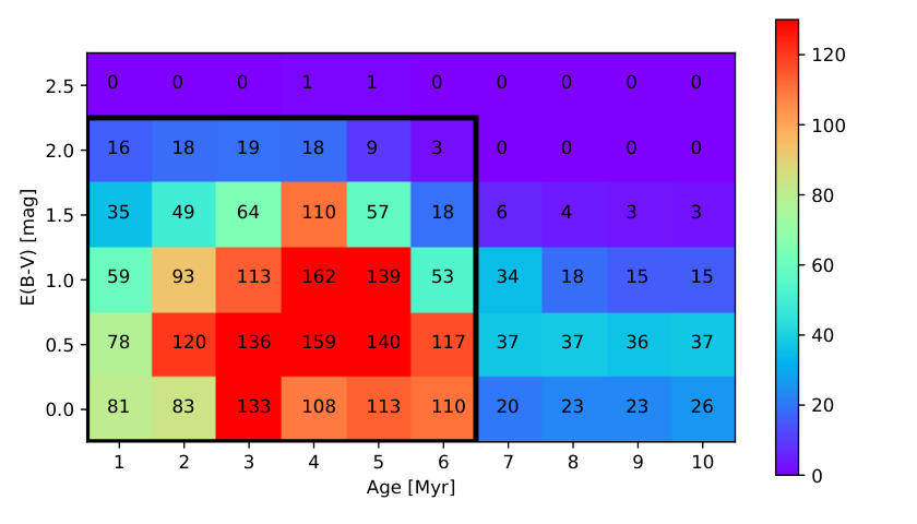
We consider the simulated sources from the completeness test described in Section IV.5 and we collect the results of their SED fitting; in Fig 15 we build a matrix showing the fraction of retrieved sources with good fits. We consider good fits the cases where the original age and extinction are consistent with the derived values within the uncertainties. The matrix proves that we have completeness above , for sources with low extinction (up to 0.5 mag). The completeness decreases to for mag and to for mag. Typically a source can be detected up to an optical depth 1, which in our case is reached for E(B–V) mag at the wavelength of Pa. Our findings are consistent with this expectation. In Fig. 16 we plot all the derived ages and masses using the method of Fig 8 and Fig. 12, in order to find if some combinations of ages and extinction are favored by the SED-fitting procedure. The figure shows that, overall, ages around 5 Myr are favored by the fitting process compared to younger ages. On the other hand, in our data we don’t see many sources with age Myr and extinctions of mag, therefore we have not over–predicted them.
Fig. 23 in Appendix B shows individual age-extinction density plots for each input age; for input ages of 4, 5 and 6 Myr we recover consistent ages, while our fitting process cannot clearly distinguish ages of 1, 2 and 3 Myr. This limitation is related to models having very similar SEDs for such young ages.
As final note, we remind that the approach used to extract our samples, limit the detection to clusters that host stars massive enough to ionised Hydrogen. As consequence, we are practically blind to clusters that do not have massive stars.

VI.2.2 Extincted sources in our samples
From our analysis we recover a total of 13 sources88 8 this total come from considering both ExtmapCat–final and PBcompact–final samples and including also the best-fit values coming from the models with differential starburst extinction. whose best fit properties fall in the ranges of ages Myr and mag. Their best fits (distributions of values and photometry) are shown in Fig. 25 and Fig. 26 in Appendix C.2. We note that not all of the best-fit values can be considered as robust, as suggested by the values, which in some cases is very high (). In particular, C10 and C307 are the two most robust cases, as their best fits follow the overall trend of the broadband SED and recover the line emission. For some other sources the least– values are small and therefore we consider the fit reasonable, but the best–fit SEDs clearly miss to reproduce the flux in one band: F547M in the case of C175–C236 (if starburst extinction is considered), F435W in the case of C251. All the other cases are less robust either because of a limited number of filters with detections (e.g. C93–C272, C187–C239, C233) or because of large least– values (e.g. C142, C228, C274). We note that all those very extincted candidates are clearly displaced from the main distribution of extinctions, that extends up to mag (see Fig. 6 and Fig. 11). In addition they all have ages between 4 and 6 Myr, while naively we would expect the most extincted sources to be the youngest. We kept all the discussed candidates in our final samples because the presence of line emission in all of them indicates they are young. However, we discuss in Section VI.3.1 how the properties of the sample would change when excluding them.
In both our samples, a fraction of the sources were not fitted due to the lack of enough photometric detections. If those were young and very extincted clusters we would be able to see their line emission, as the extinction has only small impact on H and Pa equivalent widths (see Fig. 4). As described in Section V.1, we take into account in our analyses all sources with high EW values, and we therefore took care to not to leave out of the final samples possible young and extincted candidates.
The completeness analysis of Section VI.2.1 suggests that we should find approximately half of the clusters with mag, if they were there. We expect proto–clusters to be deeply embedded into their natal cloud of gas and dust; such sources can only be seen through their MIR–FIR emission, and their investigation is beyond the scope of this study. However, we expect them to start forming massive stars and later to clear their cloud. Different concurrent factors may cause the absence of young sources with color excess in the range mag. First of all, it could simply be the case that our data are not sufficiently deep for the observation of such sources. The completeness analysis just discussed, however, rules out this possibility, as even if there is incompleteness for high extinctions, we still should be able to observe half of the clusters with mag. We remind that the comparison to the Spitzer and to the CO emission maps revealed some compact regions missed by our extinction map and therefore by our source selection. Such regions could be associated to proto-stars/proto-clusters. If this is the case, their study at high spatial resolution will be made possible by the advent of the James Webb Space Telescope.
Another possibility is that GMCs in NGC 1313 have low surface densities, and consequently clusters form in relatively low–density environments. The extinction map derived in Section III (see Fig. 1) indeed suggests that the most extincted regions of the nebular emission have mag, consistent with the high–end of the color-excess main distributions at mag derived in Section V (see Fig. 6 and 11). An observed color excess mag corresponds to a gas screen with density of (following the prescription by Bohlin et al. 1978 adjusting for sub–solar metallicity); this estimate assumes a gas screen only between the source and the observer and constitute therefore only a lower-limit estimate. ALMA observations indicate that CO clouds in NGC1313 have surface densities ranging from to , with median value (a detailed description of the ALMA observation in NGC1313 and its analysis will be presented in a coming paper, Finn et al., in prep.), consistent with the expectations estimated from the color excess and confirming the hypothesis of clusters form in relatively low–density environments.
Finally, lack of embedded clusters could be due to (or enhanced by) an extremely short duration of the process of gas clearing due to feedback after the massive stars are formed (as suggested by e.g. Matthews et al. 2018; Hannon et al. 2019; Kruijssen et al. 2019; Chevance et al. 2020a). We discuss in the next section the typical timescales associated with the clearing of the natal gas cloud. We point out that in the case of non–uniform clouds and therefore in the presence of holes that give clear lines of sight into the cluster, the fit values will tend to show lower extinction. Such patchy clouds could still be the effect of stellar feedback since early times (Dale et al. 2014, see e.g.).
VI.3 Typical cluster extinctions at young ages
VI.3.1 Distribution of extinctions
We consider in Fig. 17 the distribution of extinctions, separating the samples in two age ranges 1 to 3 and 4 to 6 Myr, to test for the presence of an age evolution. The median values are 0.31 and 0.15 mag for ExtmapCat–final and 0.28 and 0.23 mag for PBcompactCat–final, for the age ranges 1-3 and 4-6 Myr, respectively. An age–dependent extinction is suggested for the first sample, with twice the color excess for the youngest age bin than the older age bin, while the second sample does not show a trend, rather consistent values between the two age bins. We note that, despite having selected the sample to contain extincted clusters, half of our sources are consistent with having relatively low extinctions, mag, corresponding to mag.
An alternative way of studying the typical extinctions of our samples is to consider the fraction of clusters below a certain limit. In Tab. 3 we report the fraction of clusters with values below 0.25 mag, , i.e. the values of the lowest row in the density plot in Fig. 8 and Fig. 12 divided by the total value in each column. These can be considered the fraction of low-extincted clusters. Once again, we separate the samples in two age bins.
The fractions varies from to for ExtmapCat–final and from to for PBcompactCat–final. As before, the ExtmapCat–final sample shows a slightly stronger age–dependent extinction trend than the other sample.
We can compare our samples to the cluster sample found by the LEGUS collaboration. We recall that the LEGUS sample selection is based on source detection in at least 4 filters in the NUV-optical range. The values of LEGUS clusters with ages Myr are shown in Fig. 18 and the fraction of low-extinction clusters are collected in Tab. 3. Both the median values, 0.10 and 0.14 mag for the 1-3 and 4-6 Myr age ranges, respectively, and the fraction of low-extinction sources, and in the two age bins, respectively, indicate lower extinctions for the LEGUS clusters compared to our sample. This suggests, as expected, that the process of the sample selection in LEGUS is biased against clusters with higher extinctions.
There are 21 sources in common between the LEGUS and our samples. We consider their distribution and fraction of low-extinction sources in Fig 18; their median values (0.22 and 0.26 mag) are consistent with the values from the overall PBcompactCat–final sample. The same is true for the fraction of low-extinction clusters (see Tab. 3). We deduce that our samples are consistent with the higher–extinction portion of the LEGUS sample, i.e. we are biased (by construction) against clusters with low-extinction. This is a direct consequence of the source selection method, that avoided regions with low extinction (in the extinction map derived in Section III.1) and sources without compact Pa emission. Similarly, clusters of our samples are not considered in LEGUS, and therefore the latter sample is biased against sources with high-extinction.
We create a “master” catalog by merging ExtmapCat–final, PBcompactCat–final and the LEGUS catalog (removing the duplicates, i.e. the sources in common). The master catalog counts 254 sources and we consider it as a more complete version of either our or the LEGUS samples; out of 208 sources with ages between 1 and 6 Myr in the “master” catalog, 76 () are found exclusively in this study and were missed by LEGUS, while for 112 () it is true the opposite. In the case of the “master” catalog, we do not find an age evolution of the median values, nor of (Fig. 19 and Tab. 4). As discussed in the previous section, most of the sources with mag are not robust results; repeating the analysis of the master catalog excluding such sources yields an age trend of both the median and . In any case, we recover overall a low typical value for the cluster extinctions, with median mag or lower.
| Sample | ||
|---|---|---|
| 1-3 Myr | 4-6 Myr | |
| ExtmapCat–final | 41% | 63% |
| PBcompactCat–final | 45% | 57% |
| LEGUS | 84% | 75% |
| LEGUS (in common) | 25% | 48% |
| Age | w/o high | |
|---|---|---|
| 1 Myr | 64% | 64% |
| 2 Myr | 67% | 67% |
| 3 Myr | 81% | 81% |
| 4 Myr | 71% | 73% |
| 5 Myr | 73% | 84% |
| 6 Myr | 68% | 87% |
| 1-3 Myr | 70% | 70% |
| 4-6 Myr | 71% | 77% |
VI.3.2 H and Pa morphology
Following the analysis of Hannon et al. 2019 we visually classify the morphology of the H and Pa emission associated with each source of our samples. We follow their same classification scheme, mediated by Whitmore et al. 2011 and Hollyhead et al. 2015 who divide the sample in 3 classes:
- 1.
concentrated, i.e. there is a compact HII region on the position of the cluster;
- 2.
partially exposed, i.e. either the HII region shows bubble–like morphology or only partially cover the cluster or emission is diffuse;
- 3.
no emission, i.e. the target cluster is not associated to any nebular emission.
This division in classes is expected to reflect an evolution of the clusters and indeed both Hollyhead et al. 2015 and Hannon et al. 2019 found an increase of the median age of clusters, when going from concentrated, to partially exposed, to no emission. We show, in Fig. 20, age and extinction distributions of the clusters in our sample (merging together sources from ExtmapCat–final and from PBcompactCat–final), separating them in the three classes above. The classification was done independently in H and in Pa, and therefore we end up with two classifications for each cluster. For both line morphologies, we find a trend with age, that have median values of 2, 4 and 6 Myr for “concentrated”, “partially exposed” and “no emission” classes, respectively. We see a possible trend with extinction in the case of Pa morphology, as median values decrease going from concentrated to no emission classes, but the same is not true in the case of H morphology. In the latter case the median extinction of the “no emission” class is driven by the group of clusters with high extinctions.
An interesting feature coming out of the plots in Fig. 20 is that the almost totality of clusters with have compact Pa emission but no H. If we assume their extinction values are correct, we expect the absence of H emission to be driven by the elevated extinction. We test this hypothesis by deriving, from the Pa line emission map (Section III.1), the Pa flux of those 7 sources and converting it into an expected H flux (taking into account the extinction of each source). The derived H fluxes span the range Å-1. In the assumption of their flux uniformly distributed over a circular region of 1 pc radius ( px at the distance of NGC 1313), their surface brightness is between 1 and 14 sigmas above the noise at their coordinates. 4 out of 7 of them have an expected H emission more than above the detection limit. The hypothesis is therefore only partially confirmed. We also note that all the 7 sources considered are found in regions far from the large star–forming sub–regions (see Fig. 7), and appear in the Pa map as isolated sources.
Assuming to have a complete catalog of cluster covering the age range 0-10 Myr, Hannon et al. 2019 estimate the timescale associated to each of the H morphological classes, by simply converting the fraction of sources in the class to a timescale in Myr. We discussed in the previous section how the LEGUS catalog that the authors used for this estimate is incomplete, being biased against extincted sources. We repeat their analysis using the master catalog created merging our final samples with the LEGUS catalog. We report in Tab. 5 the timescales for each morphological stage, for the LEGUS sample (of NGC1313 only, while Hannon et al. 2019 reported the value calculated considering together 3 of the LEGUS galaxies), for our final samples alone and for the merged sample. In the case of our samples alone, we assume that they are representative of the age range 0-6 Myr, while for the other two samples we consider an age range 0-10 Myr. The addition of our samples to the LEGUS one prolongs the timescale of the “concentrated” stage from Myr to Myr, while the intermediate stage of partial emission remains Myr long. We conclude that already at Myr, the HII regions typically begin to disperse, and by Myr there is very little or no nebular emission left around the clusters in NGC 1313.
| Sample | Age Range | |||||
|---|---|---|---|---|---|---|
| Concentrated | Partial emission | No emission | ||||
| Hannon et al. 2019 | 19.1% | 1.9 Myr | 16.3% | 1.6 Myr | 64.6% | 6.5 Myr |
| This work | 65.6% | 3.9 Myr | 25.0% | 1.5 Myr | 9.4% | 0.6 Myr |
| Merged | 30.6% | 3.1 Myr | 18.4% | 1.8 Myr | 51.0% | 5.1 Myr |
VII Summary and conclusions
Using NUV–optical–NIR HST broad and narrow–band observations of the nearby galaxy NGC 1313 we looked for young and embedded star clusters. In particular, new NIR data are used to derive a map of the Paschen nebular emission and to characterize extincted sources possibly missed by previous analysis focused on the NUV-optical part of the spectrum.
We extract a catalog of possible candidates in two different ways:
- 1.
the first selection is made by using a map of nebular extinction derived from H and Pa observations. Sub–regions of the galaxy where the extinction is higher than mag were searched for sources in the F814W filter with counterparts in the NIR filters;
- 2.
with a complementary approach, we select sources with compact Pa emission within the entire galaxy.
The sources in the two resulting catalogs, named ExtmapCat and PBcompactCat respectively, are analyzed photometrically and via a least- broad and narrow–band SED fit, in order to derive their ages, masses and extinctions. The effective radius of each source is estimated assuming a spherical symmetrical Moffat profile; most of the sources in the initial catalogs have a light profile consistent with stars. Among the star–like sources, only the ones with H and Pa equivalent widths higher than Åand Årespectively, i.e. consistent with being younger than 6 Myr according to our models (see Section IV.4) are retained in the final samples. In addition, only sources with small uncertainties in the derived ages are considered in the final samples.
The final samples count 46 and 84 sources for ExtmapCat–final and PBcompactCat–final respectively. 30 clusters are in common among the two final catalogs. The median size of the sources in the final samples is pc (Fig. 13). Overall, they are mainly distributed in the age range Myr, with extinctions mag and masses in the range (Fig. 6 and Fig. 11). The ages derived via the broad–band SED fit are consistent with the ages that would be estimated from the H and Pa equivalent widths values (Fig. 5 and Fig. 10). A comparison between models with various metallicities and extinction curves reveals that clusters in NGC 1313 are better fit by models with sub–solar metallicity, , and Milky Way extinction curve (Fig. 9, Fig. 12 and Fig. 24).
In addition to use the results from photometry and SED fitting, we classify the morphology of the H and Pa emission associated to each of the sources in the final samples; following the example of previous studies (Whitmore et al. 2011; Hollyhead et al. 2015; Hannon et al. 2019, e.g.), we used a 3–classes division, namely “concentrated” nebular emission, “partially exposed” and sources with “no (nebular) emission” associated. The classes are assumed to describe the time evolution of the gas from a dense cloud to the dispersion. Most of the sources in our final samples fall into the first class, especially for what concerns the Pa emission; we remind that the PBcompactCat sample is expected to contain sources with concentrated Pa emission, by construction.
Despite the majority of the sources in the final catalogs having low extinctions, for 13 sources we derived mag. Not all of their fits are robust; in some cases the associated to the best fit are high (), in some other cases we have detections only in a few () filters. Several of these sources have concentrated Pa emission but no H detected (Fig. 20); based on their Pa flux and their derived values more than half of them should have H detectable. In addition, they are located far from the main star–forming regions (Fig. 7). Overall, we consider them only as possible candidates for young and extincted regions. Only two of them (with slightly above 1.0 mag) have robust fits.
We expect the young clusters to form in dense clouds of gas and dust, and to be still embedded in their natal cloud at birth. We propose a few hypotheses for the small number of young and extincted sources observed.
- •
Low surface densities of the GMCs hosting star formation. An extinction of mag would correspond to a gas screen with a surface density of , consistent with the average values for GMCs in NGC 1313 as revealed by ALMA observations.
- •
An extremely short timescale for the clearing of the natal cloud due to feedback, on the order of Myr; short timescales could be related to low gas surface density discussed in the previous point.
- •
Via a completeness test, we estimate an incompleteness of at mag (see Fig. 15). According to this test, we would expect to recover of the sources with between and mag but we found only one source in such extinction range and with age Myr (out of 45 total sources with age Myr found).
We study the distribution of extinction in function of cluster ages, expecting younger sources to be more extincted.
- •
We recover a weak dependence of with age (Fig. 17); of the sources with ages in the range Myr have mag, while the percentage rise to for the sources with ages Myr. These data confirm that a significant fraction of sources have low extinction already at ages Myr.
- •
A clear trend is observed between the morphology of the Pa emission and the age and extinction of the relative cluster; sources with concentrated emission are on average younger and more extincted than sources with partial or no emission (Fig. 5).
We include the clusters from the LEGUS catalog (focused on NUV-optical sources, while our catalogs are focused on optical-NIR) to create a “master” catalog, more representative of the entire young cluster population of NGC 1313.
- •
Repeating the study of the extinctions on the master catalog, we find weak or no evolution with age, depending on whether the sources with mag discussed above are excluded from consideration or not. (Fig. 19). At best, of the clusters with ages Myr have low extinctions (below ) with the percentage rising to in the age range Myr.
- •
Assuming that the “master” sample is representative of the NGC 1313 cluster population in the age range Myr we use the fraction of sources in each class to estimate its typical timescale. We recover Myr for the concentrated phase, Myr for the “partial emission” and Myr for the “no emission” phase. This results prolongs the expected timescale for clearing the cloud by Myr () compared to a previous estimate based only on NUV–optical data.
Clusters in NGC 1313 appear to have cleared the gas cloud around them by the time they reach an age of Myr and many of them are already almost gas free within the first 3 Myr. We conclude that the inclusion of a tracer more transparent to extinction (NIR observations) has allowed to recover the fraction of clusters that are missed in optical–NUV studies and better pin down previous estimates of the duration of the embedded phase to Myr; including young embedded clusters in NGC 1313 changes previous estimates of the short feedback timescales from clusters by (from Myr to Myr), bringing it closer to the timescales for the first supernova explosions, which could occur as early as Myr (Sukhbold et al. 2016, e.g.). In addition, photoionisation, radiation pressure and winds can open channels before supernovae explode for low mass GMCs (, e.g. Dale et al. 2014; Dale 2015).
The analysis also suggested that the median age of the cluster correlates better with the morphology of the nebular emission (Fig. 20) than with the cluster extinction (Fig. 17 and Fig. 19); we deduce that the H (and Pa) morphology is a good tracer of the cluster age evolution. On the other hand, median cluster extinctions also show some correlation with the ionized gas morphology (Fig. 20) but also reveal that many clusters with ’concentrated’ nebular emission associated are not very extincted, with mag, i.e. even when a cluster is still surrounded by a compact gas cloud, its effect on the cluster extinction can be low. We speculate that this could be caused by non-uniform gas–dust clouds, where holes in the line–of–sight direction allow the escape of the stellar radiation.
We point out that the current study consider only clusters in NGC 1313, a single galaxy with a given metallicity (best estimate: ) and SFR density (). In addition, most of the clusters masses in NGC 1313 are distributed around a mass of . We plan in the near future to extend this study to galaxies with different properties and clusters with wider range of masses, in order to estimate if and how the interaction between the very young clusters and their cloud is affected by the host galaxy properties and by the properties of cluster themselves.
References
- Adamo et al. (2015) Adamo, A., Kruijssen, J. M. D., Bastian, N., Silva-Villa, E., & Ryon, J. 2015, MNRAS, 452, 246, doi: 10.1093/mnras/stv1203
- Adamo et al. (2010) Adamo, A., Zackrisson, E., Östlin, G., & Hayes, M. 2010, ApJ, 725, 1620, doi: 10.1088/0004-637X/725/2/1620
- Adamo et al. (2017) Adamo, A., Ryon, J. E., Messa, M., et al. 2017, ApJ, 841, 131, doi: 10.3847/1538-4357/aa7132
- Aversa et al. (2011) Aversa, A. G., Johnson, K. E., Brogan, C. L., Goss, W. M., & Pisano, D. J. 2011, AJ, 141, 125, doi: 10.1088/0004-6256/141/4/125
- Bastian et al. (2013) Bastian, N., Schweizer, F., Goudfrooij, P., Larsen, S. S., & Kissler-Patig, M. 2013, MNRAS, 431, 1252, doi: 10.1093/mnras/stt253
- Bastian et al. (2012) Bastian, N., Adamo, A., Gieles, M., et al. 2012, MNRAS, 419, 2606, doi: 10.1111/j.1365-2966.2011.19909.x
- Bohlin et al. (1978) Bohlin, R. C., Savage, B. D., & Drake, J. F. 1978, ApJ, 224, 132, doi: 10.1086/156357
- Calzetti et al. (2000) Calzetti, D., Armus, L., Bohlin, R. C., et al. 2000, ApJ, 533, 682, doi: 10.1086/308692
- Calzetti et al. (2015a) Calzetti, D., Johnson, K. E., Adamo, A., et al. 2015a, ApJ, 811, 75, doi: 10.1088/0004-637X/811/2/75
- Calzetti et al. (2015b) Calzetti, D., Lee, J. C., Sabbi, E., et al. 2015b, AJ, 149, 51, doi: 10.1088/0004-6256/149/2/51
- Cardelli et al. (1989) Cardelli, J. A., Clayton, G. C., & Mathis, J. S. 1989, ApJ, 345, 245, doi: 10.1086/167900
- Chandar et al. (2015) Chandar, R., Fall, S. M., & Whitmore, B. C. 2015, ApJ, 810, 1, doi: 10.1088/0004-637X/810/1/1
- Chevance et al. (2020a) Chevance, M., Kruijssen, J. M. D., Hygate, A. P. S., et al. 2020a, MNRAS, 493, 2872, doi: 10.1093/mnras/stz3525
- Chevance et al. (2020b) Chevance, M., Kruijssen, J. M. D., Vazquez-Semadeni, E., et al. 2020b, Space Sci. Rev., 216, 50, doi: 10.1007/s11214-020-00674-x
- Corbelli et al. (2017) Corbelli, E., Braine, J., Bandiera, R., et al. 2017, A&A, 601, A146, doi: 10.1051/0004-6361/201630034
- Dale (2015) Dale, J. E. 2015, New A Rev., 68, 1, doi: 10.1016/j.newar.2015.06.001
- Dale et al. (2014) Dale, J. E., Ngoumou, J., Ercolano, B., & Bonnell, I. A. 2014, MNRAS, 442, 694, doi: 10.1093/mnras/stu816
- de Vaucouleurs (1963) de Vaucouleurs, G. 1963, ApJ, 137, 720, doi: 10.1086/147550
- Elmegreen & Elmegreen (2019) Elmegreen, B. G., & Elmegreen, D. M. 2019, ApJS, 245, 14, doi: 10.3847/1538-4365/ab4903
- Elmegreen & Elmegreen (2020) —. 2020, ApJ, 895, 71, doi: 10.3847/1538-4357/ab8d20
- Elmegreen et al. (2018) Elmegreen, B. G., Elmegreen, D. M., & Efremov, Y. N. 2018, ApJ, 863, 59, doi: 10.3847/1538-4357/aacf9a
- Elson et al. (1987) Elson, R. A. W., Fall, S. M., & Freeman, K. C. 1987, ApJ, 323, 54, doi: 10.1086/165807
- Ferland et al. (2013) Ferland, G. J., Porter, R. L., van Hoof, P. A. M., et al. 2013, Rev. Mexicana Astron. Astrofis., 49, 137. https://arxiv.org/abs/1302.4485
- Finn et al. (2019) Finn, M. K., Johnson, K. E., Brogan, C. L., et al. 2019, ApJ, 874, 120, doi: 10.3847/1538-4357/ab0d1e
- Fitzpatrick (1999) Fitzpatrick, E. L. 1999, PASP, 111, 63, doi: 10.1086/316293
- Gaia Collaboration et al. (2018) Gaia Collaboration, Brown, A. G. A., Vallenari, A., et al. 2018, A&A, 616, A1, doi: 10.1051/0004-6361/201833051
- Grasha et al. (2017a) Grasha, K., Elmegreen, B. G., Calzetti, D., et al. 2017a, ApJ, 842, 25, doi: 10.3847/1538-4357/aa740b
- Grasha et al. (2017b) Grasha, K., Calzetti, D., Adamo, A., et al. 2017b, ApJ, 840, 113, doi: 10.3847/1538-4357/aa6f15
- Grasha et al. (2018) Grasha, K., Calzetti, D., Bittle, L., et al. 2018, MNRAS, 481, 1016, doi: 10.1093/mnras/sty2154
- Grasha et al. (2019) Grasha, K., Calzetti, D., Adamo, A., et al. 2019, MNRAS, 483, 4707, doi: 10.1093/mnras/sty3424
- Hannon et al. (2019) Hannon, S., Lee, J. C., Whitmore, B. C., et al. 2019, MNRAS, 490, 4648, doi: 10.1093/mnras/stz2820
- Hollyhead et al. (2015) Hollyhead, K., Bastian, N., Adamo, A., et al. 2015, MNRAS, 449, 1106, doi: 10.1093/mnras/stv331
- Jacobs et al. (2009) Jacobs, B. A., Rizzi, L., Tully, R. B., et al. 2009, AJ, 138, 332, doi: 10.1088/0004-6256/138/2/332
- Johnson et al. (2018) Johnson, K. E., Brogan, C. L., Indebetouw, R., et al. 2018, ApJ, 853, 125, doi: 10.3847/1538-4357/aa9ff8
- Johnson et al. (2009) Johnson, K. E., Hunt, L. K., & Reines, A. E. 2009, AJ, 137, 3788, doi: 10.1088/0004-6256/137/4/3788
- Johnson et al. (2004) Johnson, K. E., Indebetouw, R., Watson, C., & Kobulnicky, H. A. 2004, AJ, 128, 610, doi: 10.1086/422017
- Johnson & Kobulnicky (2003) Johnson, K. E., & Kobulnicky, H. A. 2003, ApJ, 597, 923, doi: 10.1086/378585
- Johnson et al. (2001) Johnson, K. E., Kobulnicky, H. A., Massey, P., & Conti, P. S. 2001, ApJ, 559, 864, doi: 10.1086/322335
- Johnson et al. (2015) Johnson, K. E., Leroy, A. K., Indebetouw, R., et al. 2015, ApJ, 806, 35, doi: 10.1088/0004-637X/806/1/35
- Johnson et al. (2016) Johnson, L. C., Seth, A. C., Dalcanton, J. J., et al. 2016, ApJ, 827, 33, doi: 10.3847/0004-637X/827/1/33
- Kennicutt et al. (2008) Kennicutt, Robert C., J., Lee, J. C., Funes, J. G., et al. 2008, ApJS, 178, 247, doi: 10.1086/590058
- Kepley et al. (2014) Kepley, A. A., Reines, A. E., Johnson, K. E., & Walker, L. M. 2014, AJ, 147, 43, doi: 10.1088/0004-6256/147/2/43
- Kewley & Dopita (2002) Kewley, L. J., & Dopita, M. A. 2002, ApJS, 142, 35, doi: 10.1086/341326
- Kobulnicky & Johnson (1999) Kobulnicky, H. A., & Johnson, K. E. 1999, ApJ, 527, 154, doi: 10.1086/308075
- Kroupa (2001) Kroupa, P. 2001, MNRAS, 322, 231, doi: 10.1046/j.1365-8711.2001.04022.x
- Kruijssen et al. (2019) Kruijssen, J. M. D., Schruba, A., Chevance, M., et al. 2019, Nature, 569, 519, doi: 10.1038/s41586-019-1194-3
- Krumholz et al. (2019) Krumholz, M. R., McKee, C. F., & Bland -Hawthorn, J. 2019, ARA&A, 57, 227, doi: 10.1146/annurev-astro-091918-104430
- Lada & Lada (2003) Lada, C. J., & Lada, E. A. 2003, ARA&A, 41, 57, doi: 10.1146/annurev.astro.41.011802.094844
- Leitherer et al. (1999) Leitherer, C., Schaerer, D., Goldader, J. D., et al. 1999, ApJS, 123, 3, doi: 10.1086/313233
- Lin et al. (2020) Lin, Z., Calzetti, D., Kong, X., et al. 2020, ApJ, 896, 16, doi: 10.3847/1538-4357/ab9106
- Matthews et al. (2018) Matthews, A. M., Johnson, K. E., Whitmore, B. C., et al. 2018, ApJ, 862, 147, doi: 10.3847/1538-4357/aac958
- Messa et al. (2019) Messa, M., Adamo, A., Östlin, G., et al. 2019, MNRAS, 487, 4238, doi: 10.1093/mnras/stz1337
- Messa et al. (2018a) —. 2018a, MNRAS, 473, 996, doi: 10.1093/mnras/stx2403
- Messa et al. (2018b) Messa, M., Adamo, A., Calzetti, D., et al. 2018b, MNRAS, 477, 1683, doi: 10.1093/mnras/sty577
- Peng et al. (2002) Peng, C. Y., Ho, L. C., Impey, C. D., & Rix, H.-W. 2002, AJ, 124, 266, doi: 10.1086/340952
- Peng et al. (2010) —. 2010, AJ, 139, 2097, doi: 10.1088/0004-6256/139/6/2097
- Peters et al. (1994) Peters, W. L., Freeman, K. C., Forster, J. R., Manchester, R. N., & Ables, J. G. 1994, MNRAS, 269, 1025, doi: 10.1093/mnras/269.4.1025
- Reines et al. (2010) Reines, A. E., Nidever, D. L., Whelan, D. G., & Johnson, K. E. 2010, ApJ, 708, 26, doi: 10.1088/0004-637X/708/1/26
- Ryon et al. (2015) Ryon, J. E., Bastian, N., Adamo, A., et al. 2015, MNRAS, 452, 525, doi: 10.1093/mnras/stv1282
- Ryon et al. (2017) Ryon, J. E., Gallagher, J. S., Smith, L. J., et al. 2017, ApJ, 841, 92, doi: 10.3847/1538-4357/aa719e
- Silva-Villa & Larsen (2012) Silva-Villa, E., & Larsen, S. S. 2012, MNRAS, 423, 213, doi: 10.1111/j.1365-2966.2012.20797.x
- Sukhbold et al. (2016) Sukhbold, T., Ertl, T., Woosley, S. E., Brown, J. M., & Janka, H. T. 2016, ApJ, 821, 38, doi: 10.3847/0004-637X/821/1/38
- Tsai et al. (2009) Tsai, C.-W., Turner, J. L., Beck, S. C., Meier, D. S., & Ho, P. T. P. 2009, AJ, 137, 4655, doi: 10.1088/0004-6256/137/6/4655
- Turner & Beck (2004) Turner, J. L., & Beck, S. C. 2004, ApJ, 602, L85, doi: 10.1086/382699
- Vacca et al. (2002) Vacca, W. D., Johnson, K. E., & Conti, P. S. 2002, AJ, 123, 772, doi: 10.1086/338644
- Vázquez & Leitherer (2005) Vázquez, G. A., & Leitherer, C. 2005, ApJ, 621, 695, doi: 10.1086/427866
- Whelan et al. (2011) Whelan, D. G., Johnson, K. E., Whitney, B. A., Indebetouw, R., & Wood, K. 2011, ApJ, 729, 111, doi: 10.1088/0004-637X/729/2/111
- Whitmore et al. (2011) Whitmore, B. C., Chandar, R., Kim, H., et al. 2011, ApJ, 729, 78, doi: 10.1088/0004-637X/729/2/78
- Zackrisson et al. (2001) Zackrisson, E., Bergvall, N., Olofsson, K., & Siebert, A. 2001, A&A, 375, 814, doi: 10.1051/0004-6361:20010912
- Zackrisson et al. (2011) Zackrisson, E., Rydberg, C.-E., Schaerer, D., Östlin, G., & Tuli, M. 2011, ApJ, 740, 13, doi: 10.1088/0004-637X/740/1/13
Appendix A Further details of the size analysis
In Section IV.2 we measure the size of clusters using a size-photometry routine; at the same time this routine allows to measure the cluster fluxes taking into account the width of their light profile, without relying on an aperture correction. In each filter the source is modelled as a convolution between the instrumental PSF , where denote the current filter, and a Moffat profile (Elson et al. 1987). In order to take a non–uniform sky background into account, the source model was added to a –degree polynomial (described by 3 parameters, , and ). The observable model (M) is therefore parametrized as:
| (A1) |
where is related to the effective radius by and the radial distance is defined as , where are the pixel coordinates and are the source coordinates. and parametrize the flux and size of the source, respectively. We point out that the PSF profile is normalized and that the Moffat profile is also normalized via the . Since nearby sources can cause contamination especially in the bluer filters, we use F814W to estimate the coordinates and the size of each of the sources. Fig. 21 shows an example from the fit of one of the clusters. The flux uncertainties are correlated with uncertainties on the other parameters, especially with the size. In order to take it into account, we repeat the fit in the F814W filter twice, the second time keeping fixed coordinates and size. We consider for each source the relative uncertainty given by the size and position uncertainties:
| (A2) |
where and are the total uncertainties on the flux uncertainties in the two repetitions of the fit. Then for every filter we use this relative value to correct the uncertainty derived from the fit with fixed size, :
| (A3) |
where is the flux measured for the current source in the filter .

Appendix B Additional plots for the completeness test
We report in Tab. 6 and Fig. 22 a summary of the completeness in detecting photometrically the input sources in the context of the completeness test described in the main text in Section IV.5 and Section VI.2.1. In Fig. 23 we report the density plot showing how the recovered ages and extinctions are distributed, for each of the input ages used. The main conclusion that can be drawn form Fig. 23 is that our age determination via broad– (and narrow–) band SED fitting is degenerate for very young ages; in fact, for the simulated clusters with age of 1 Myr, we retrieved estimated ages equally split between 1 and 2 Myr. Similarly the estimated ages for the simulated clusters of 2 Myr span the entire range up to 3 Myr with almost constant frequency. Only for simulated clusters with ages of 4 Myr (and older) the SED fitting returns consistent ages, with little age spread. This effect is mainly caused by the stellar models used being very similar with each other for young ages, causing degeneracy in the SED fitting process. For this reason, in the main text we consider as degenerate the SEDs with ages of 3 Myr and below.
| Age | E(B-V) F814W | E(B-V) F128N | ||||||||
|---|---|---|---|---|---|---|---|---|---|---|
| 0.0 | 0.5 | 1.0 | 1.5 | 2.0 | 0.0 | 0.5 | 1.0 | 1.5 | 2.0 | |
| 1 Myr | 100 | 100 | 99 | 95 | 86 | 99 | 98 | 99 | 99 | 98 |
| 2 Myr | 100 | 100 | 99 | 97 | 80 | 100 | 100 | 99 | 100 | 96 |
| 3 Myr | 100 | 99 | 100 | 92 | 85 | 100 | 99 | 99 | 93 | 93 |
| 4 Myr | 100 | 99 | 100 | 94 | 84 | 99 | 97 | 98 | 90 | 86 |
| 5 Myr | 100 | 99 | 100 | 95 | 75 | 98 | 97 | 90 | 92 | 73 |
| 6 Myr | 100 | 100 | 100 | 97 | 90 | 97 | 97 | 96 | 85 | 82 |


Appendix C Individual fit results
We report in this section the plots of the SED fitting process for some of the sources discussed in the main text.
C.1 Comparing solar and sub-solar metallicities
We show in Fig. 24 some examples of the observed broad-band SED of young sources with line emission and the best-fit SED values using solar and sub-solar metallicites. While in both cases the best-fit values for the ages denote young sources (), the models with sub-solar metallicity are more capable of capturing the flux difference observed between the F555W and the F547M filters. Also the values of the best in the two cases confirm this trend.
C.2 young and extincted candidates
We show in Fig. 25 and Fig. 26 the sources whose best fit results suggest them being young and extincted. The single cases are discussed in Section VI.2.2.


