跳到论文正文
W Papers独立论文阅读器 arXiv:2011.09356 论文正文 计算阅读时间 · 0%
引用这篇论文根据当前论文元数据生成,正式投稿前建议核对。


License: arXiv.org perpetual non-exclusive license
arXiv:2011.09356v2 [math.PR] 19 Oct 2021

Limits and fluctuations of pp-adic random matrix productsThanks: I thank my advisor Alexei Borodin for many helpful conversations throughout this project and feedback on several drafts; Vadim Gorin, for early encouragement, pointers to the matrix product literature, and other helpful discussions and comments; and Andrew Ahn, for many illuminating discussions on the complex case and its relation to this work, and detailed feedback on the exposition. Some preliminary material appeared in my unpublished undergraduate thesis [60], and it is my pleasure to thank Ju-Lee Kim for her guidance on that project. I also wish to thank Adam Block, Jason Fulman, Nathan Kaplan, Mario Kieburg, Sergei Korotkikh, and Kevin Lin for additional helpful conversations. This material is based on work supported by the National Science Foundation Graduate Research Fellowship under Grant No. #17453021745302.

Roger Van Peski
Date: August 11, 2026
Abstract.

We show that singular numbers (also known as elementary divisors, invariant factors or Smith normal forms) of products and corners of random matrices over ℚp\mathbb{Q}_{p} are governed by the Hall-Littlewood polynomials, in a structurally identical manner to the known relations between singular values of complex random matrices and Heckman-Opdam hypergeometric functions. This implies that the singular numbers of a product of corners of Haar-distributed elements of GLN​(ℤp)\mathrm{GL}_{N}(\mathbb{Z}_{p}) form a discrete-time Markov chain distributed as a Hall-Littlewood process, with the number of matrices in the product playing the role of time. We give an exact sampling algorithm for the Hall-Littlewood processes which arise by relating them to an interacting particle system similar to PushTASEP. By analyzing the asymptotic behavior of this particle system, we show that the singular numbers of such products obey a law of large numbers and their fluctuations converge dynamically to independent Brownian motions. In the limit of large matrix size, we also show that the analogues of the Lyapunov exponents for matrix products have universal limits within this class of GLN​(ℤp)\mathrm{GL}_{N}(\mathbb{Z}_{p}) corners.

Key words and phrases: 
pp-adic random matrices, Hall-Littlewood polynomials, particle systems
1991 Mathematics Subject Classification
15B52 (primary); 15B33, 60B20 (secondary)

Keywords:

Mathematics Subject Classification (2020):

1. Introduction

1.1. Asymptotic results.

For any nonsingular complex matrix A∈Mn×m​(ℂ)A\in M_{n\times m}(\mathbb{C}), by singular value decomposition there exist U∈U⁡(n),V∈U⁡(m)U\in U(n),V\in U(m) with U​A​V=diag⁡(e−r1,e−r2,…,e−rmin⁡(m,n))UAV=\diag(e^{-r_{1}},e^{-r_{2}},\ldots,e^{-r_{\min(m,n)}}) for some ∞>r1≥⋯≥rmin⁡(m,n)\infty>r_{1}\geq\cdots\geq r_{\min(m,n)}. Studying the distributions of the singular values of various random matrices AA, and their asymptotics, is a classical but still very active line of research.

For any nonsingular pp-adic matrix11 1 For background on the pp-adic numbers and matrix groups over them, see Section 3. A∈Mn×m​(ℚp)A\in M_{n\times m}(\mathbb{Q}_{p}), there similarly exist U∈GLn⁡(ℤp),V∈GLm⁡(ℤp)U\in\GL_{n}(\mathbb{Z}_{p}),V\in\GL_{m}(\mathbb{Z}_{p}) such that U​A​V=diag⁡(pλ1,pλ2,…,pλmin⁡(m,n))UAV=\diag(p^{\lambda_{1}},p^{\lambda_{2}},\ldots,p^{\lambda_{\min(m,n)}}) for some integers ∞>λ1≥…≥λmin⁡(m,n)\infty>\lambda_{1}\geq\ldots\geq\lambda_{\min(m,n)}. We refer to the integers λi\lambda_{i} as the singular numbers of AA and write SN⁡(A)=(λ1,…,λmin⁡(m,n))=λ\SN(A)=(\lambda_{1},\ldots,\lambda_{\min(m,n)})=\lambda in the above case. One can study the distribution of SN⁡(A)\SN(A) for random A∈Mn×m​(ℚp)A\in M_{n\times m}(\mathbb{Q}_{p}) just as with singular values.

Such distributions have received significant attention within number theory, starting with the 1987 work of Friedman-Washington [34]. They computed the n→∞n\to\infty limiting distribution of SN⁡(A)\SN(A) for A∈Mn​(ℤp)A\in M_{n}(\mathbb{Z}_{p}) with iid entries distributed according to the additive Haar measure on ℤp\mathbb{Z}_{p}, which may be viewed as the analogue of the Gaussian in this setting. They found that it matched the distribution of the pp-torsion parts of class groups22 2 Here we view AA as a map ℤpn→ℤpn\mathbb{Z}_{p}^{n}\to\mathbb{Z}_{p}^{n} and identify λ=SN⁡(A)\lambda=\SN(A) with the abelian pp-group coker⁡(A)≅⨁iℤ/pλi​ℤ\coker(A)\cong\bigoplus_{i}\mathbb{Z}/p^{\lambda_{i}}\mathbb{Z}. of quadratic imaginary number fields conjectured by Cohen and Lenstra [23] in 1983 on the basis of numerical data, and gave a heuristic explanation why this was the case. This launched many subsequent works on modeling groups appearing in number theory by suitable random pp-adic matrices, see for instance Achter [1], Bhargava-Kane-Lenstra-Poonen-Rains [12], Ellenberg-Jain-Venkatesh [28], Wood [61, 63] and particularly the survey [62].

The asymptotic distributions obtained in the above works look quite different from their counterparts in the world of singular values. For instance, [34] show that for any nonnegative integers λ1≥λ2≥…≥0\lambda_{1}\geq\lambda_{2}\geq\ldots\geq 0 and random An∈Mn​(ℤp)A_{n}\in M_{n}(\mathbb{Z}_{p}) as above, one has

limn→∞Pr⁡(SN⁡(An)=λ)=(p−1,p−1)∞|Aut⁡(⨁iℤ/pλi​ℤ)|.\lim_{n\to\infty}\Pr(\SN(A_{n})=\lambda)=\frac{(p^{-1};p^{-1})_{\infty}}{\left\lvert\Aut(\bigoplus_{i}\mathbb{Z}/p^{\lambda_{i}}\mathbb{Z})\right\rvert}.

In particular, the limiting λi\lambda_{i} are integers, and with probability 11 only a finite number of the λi\lambda_{i} are nonzero. The motivating questions in number theory concern group-theoretic properties such as the probability of cyclicity (i.e. probability that SN⁡(A)=(k,0,…,0)\SN(A)=(k,0,\ldots,0) for some kk) or the distribution of ranks (the number of nonzero parts of λ=SN⁡(A)\lambda=\SN(A)).

By contrast, the singular values of an n×nn\times n matrix with iid standard Gaussian entries, usually referred to as the Ginibre ensemble, converge with rescaling to the celebrated Marchenko-Pastur law [49] (a compactly supported probability distribution on ℝ\mathbb{R}). As far as we are aware, no continuous probability distributions on ℝ\mathbb{R} appeared previously governing limits of singular numbers of random pp-adic matrices. Indeed, such limits are in a sense orthogonal to the viewpoint of random abelian pp-groups taken in most of the previous literature.

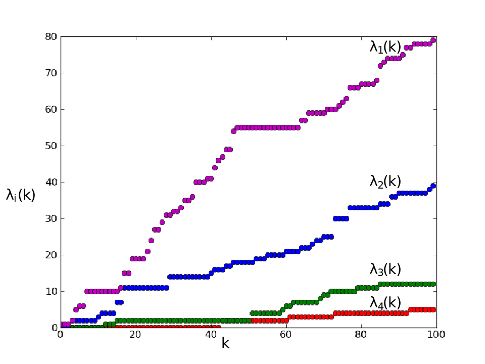
In this work we find Gaussian limits in the setting of products of a large number of pp-adic matrices of finite size. Given random matrices A1,A2,…∈Mn​(ℚp)A_{1},A_{2},\ldots\in M_{n}(\mathbb{Q}_{p}), one may view the SN⁡(A1),SN⁡(A2​A1),…\SN(A_{1}),\SN(A_{2}A_{1}),\ldots as defining a discrete-time Markov chain on the set of weakly decreasing nn-tuples of integers. Equivalently, for each ii the it​hi^{th} largest singular number evolves as some random walk on ℤ\mathbb{Z}, with the nn such random walks sometimes colliding but never crossing. See Figure 1 below.

In the case when AiA_{i} are n×nn\times n corners of independent Haar-distributed elements of GLN⁡(ℤp)\GL_{N}(\mathbb{Z}_{p}) with N>nN>n, we show that the singular numbers of their products satisfy an explicit law of large numbers as k→∞k\to\infty, and furthermore the fluctuations converge to nn independent Brownian motions. In the limit as N→∞N\to\infty, the entries of such corners become independent and distributed according to the additive Haar measure on ℤp\mathbb{Z}_{p}, recovering the matrices studied in the previous literature, so we allow the case ‘N=∞N=\infty’ below.

Theorem 1.1.

Fix n≥1n\geq 1, and let N1,N2,…∈ℤ∪{∞}N_{1},N_{2},\ldots\in\mathbb{Z}\cup\{\infty\} with Nj>nN_{j}>n for all jj. For each jj, if Nj<∞N_{j}<\infty let AjA_{j} be the top left n×nn\times n corner of a Haar distributed element of GLNj⁡(ℤp)\GL_{N_{j}}(\mathbb{Z}_{p}), and if Nj=∞N_{j}=\infty let AjA_{j} have iid entries distributed by the additive Haar measure on ℤp\mathbb{Z}_{p}. For k∈ℕk\in\mathbb{N} let

(λ1(k),…,λn(k)):=SN(Ak⋯A1).(\lambda_{1}(k),\ldots,\lambda_{n}(k)):=\SN(A_{k}\cdots A_{1}).

Then we have a strong law of large numbers

λi​(k)∑j=1k∑ℓ=0Nj−n−1p−i−ℓ​(1−p−1)(1−p−i−ℓ−1)​(1−p−i−ℓ)→1​ a.s. as k→∞.\frac{\lambda_{i}(k)}{\sum_{j=1}^{k}\sum_{\ell=0}^{N_{j}-n-1}\frac{p^{-i-\ell}(1-p^{-1})}{(1-p^{-i-\ell-1})(1-p^{-i-\ell})}}\to 1\text{ a.s. as $k\to\infty$.}

Let

λ¯i​(k):=λi​(k)−∑j=1k∑ℓ=0Nj−n−1p−i−ℓ​(1−p−1)(1−p−i−ℓ−1)​(1−p−i−ℓ){\bar{\lambda}}_{i}(k):=\lambda_{i}(k)-\sum_{j=1}^{k}\sum_{\ell=0}^{N_{j}-n-1}\frac{p^{-i-\ell}(1-p^{-1})}{(1-p^{-i-\ell-1})(1-p^{-i-\ell})}

and define the random function of fλ¯i,k∈C⁡[0,1]f_{{\bar{\lambda}}_{i},k}\in C[0,1] as follows: set fλ¯i,k​(0)=0f_{{\bar{\lambda}}_{i},k}(0)=0 and

(fλ¯i,k​(1/k),fλ¯i,k​(2/k),…,fλ¯i,k​(1))=1∑j=1k∑ℓ=0Nj−n−1p−i−ℓ​(1−p−1)​(1−p−2​i−2​ℓ−1)(1−p−i−ℓ)2​(1−p−i−ℓ−1)2​(λ¯i​(1),…,λ¯i​(k)),(f_{{\bar{\lambda}}_{i},k}(1/k),f_{{\bar{\lambda}}_{i},k}(2/k),\ldots,f_{{\bar{\lambda}}_{i},k}(1))=\frac{1}{\sqrt{\sum_{j=1}^{k}\sum_{\ell=0}^{N_{j}-n-1}\frac{p^{-i-\ell}(1-p^{-1})(1-p^{-2i-2\ell-1})}{(1-p^{-i-\ell})^{2}(1-p^{-i-\ell-1})^{2}}}}({\bar{\lambda}}_{i}(1),\ldots,{\bar{\lambda}}_{i}(k)),

then linearly interpolate from these values on each interval [ℓ/k,(ℓ+1)/k][\ell/k,(\ell+1)/k]. Then as k→∞k\to\infty, the nn-tuple of random functions (fλ¯1,k,…,fλ¯n,k)(f_{{\bar{\lambda}}_{1},k},\ldots,f_{{\bar{\lambda}}_{n},k}) converges in law in the sup norm topology on C⁡[0,1]C[0,1] to nn independent standard Brownian motions.
Refer to caption
Figure 1. A plot of (λ1(k),λ2(k),λ3(k),λ4(k))=SN(Ak⋯A1)(\lambda_{1}(k),\lambda_{2}(k),\lambda_{3}(k),\lambda_{4}(k))=\SN(A_{k}\cdots A_{1}) where A1,…,A100∈M4​(ℤ2)A_{1},\ldots,A_{100}\in M_{4}(\mathbb{Z}_{2}) are random matrices with iid entries drawn from the additive Haar measure on ℤ2\mathbb{Z}_{2}.

In particular, we have the central limit theorem that

λ¯i​(k)∑j=1k∑ℓ=0Nj−n−1p−i−ℓ​(1−p−1)​(1−p−2​i−2​ℓ−1)(1−p−i−ℓ)2​(1−p−i−ℓ−1)2→𝒩⁡(0,1)\frac{{\bar{\lambda}}_{i}(k)}{\sqrt{\sum_{j=1}^{k}\sum_{\ell=0}^{N_{j}-n-1}\frac{p^{-i-\ell}(1-p^{-1})(1-p^{-2i-2\ell-1})}{(1-p^{-i-\ell})^{2}(1-p^{-i-\ell-1})^{2}}}}\to\mathcal{N}(0,1)

in law for each ii.

Remark 1.

If all NjN_{j} are equal to some NN, then the law of large numbers takes the more standard form

λi​(k)k→∑ℓ=0N−n−1p−i−ℓ​(1−p−1)(1−p−i−ℓ−1)​(1−p−i−ℓ).\frac{\lambda_{i}(k)}{k}\to\sum_{\ell=0}^{N-n-1}\frac{p^{-i-\ell}(1-p^{-1})}{(1-p^{-i-\ell-1})(1-p^{-i-\ell})}.

When N=∞N=\infty, evaluating the sum via the qq-Gauss identity [45, (3.5)] yields an even more explicit limit:

λi​(k)k→1pi−1.\frac{\lambda_{i}(k)}{k}\to\frac{1}{p^{i}-1}.

The matrices AiA_{i} above lie in GLn⁡(ℚp)\GL_{n}(\mathbb{Q}_{p}) with probability 11, so 1.1 may be viewed as a statement about certain random walks on the group GLn⁡(ℚp)\GL_{n}(\mathbb{Q}_{p}). Previous work by Brofferio-Schapira [17] takes this perspective of random walks on groups and studies similar random walks from an ergodic theory perspective. They prove a law of large numbers for products of iid random matrices from a quite general class of probability distributions on GLn⁡(ℚp)\GL_{n}(\mathbb{Q}_{p}) via a generalization of Oseledets’ multiplicative ergodic theorem [53] to matrices over ℚp\mathbb{Q}_{p}, due to Raghunathan [55]. The family of probability distributions considered in [17] is more general than that of 1.3, but the latter covers cases when the matrices AiA_{i} are not identically distributed and shows Gaussian fluctuations, which are not shown in [17]. A different family of random walks on GLn⁡(ℚp)\GL_{n}(\mathbb{Q}_{p}) were studied by Chhaibi [22]; the perspective in this work is more similar to ours in that it is heavily based on special functions on pp-adic groups, though the presentation and problems considered are quite different. Finally, there is a body of work on random walks on Bruhat-Tits buildings which translates to results on random walks on pp-adic groups, see for instance Cartwright-Woess [21, Section 8], Schapira [56], and especially the survey of Parkinson [54]. These works contain central limit theorems, but for quite different quantities and settings than ours.

In the setting of real and complex matrices, the study of asymptotics of singular values of products AkAk−1⋯A1A_{k}A_{k-1}\cdots A_{1} of random matrices as k→∞k\to\infty dates back at least as far as the 1960 work of Furstenberg and Kesten [38], who showed Gaussian fluctuations for the logarithm of the largest singular value under some assumptions on the AiA_{i}. In the case where the AiA_{i} are iid square with complex Gaussian entries, Gaussian fluctuations for logarithms of all singular values (not just the largest as in [38]) were obtained in the physics literature by Akemann-Burda-Kieburg [5] and in the mathematics literature by Liu-Wang-Wang [46, Thm. 1.1]. The case of products of n×nn\times n corners of unitary matrices, often referred to as the truncated unitary ensemble, has also been considered; the term Jacobi ensemble is also sometimes used for such corners due to the relation with the classical Jacobi orthogonal polynomial ensemble. Dynamical convergence of the logarithm of the largest singular value of Ak⋯A1A_{k}\cdots A_{1} to Brownian motion for products of such unitary corners is suggested, though not directly implied, by the work of Ahn (one should send T^→∞\hat{T}\to\infty in [2, Thm. 1.7]). Together these results strongly suggest that as the number of products goes to infinity, the fluctuations of the nn log-singular values should converge to nn independent Brownian motions, as holds in the pp-adic case by 1.1, but this full result has to our knowledge not appeared.

There is now a large body of both mathematics and physics literature on asymptotics of matrix products in various regimes, often from the perspective of ergodic theory and often motivated by connections to chaotic dynamical systems and disordered systems in statistical physics, neural networks, and other areas. See for example Ahn [2, 3], Akemann-Burda-Kieburg [5, 6, 7], Akemann-Ipsen [8], Akemann-Ipsen-Kieburg [9], Akemann-Kieburg-Wei [10], Crisanti-Paladin-Vulpiani [26], Forrester [31] and Forrester-Liu [32], Gol’dsheid-Margulis [39], Gorin-Sun [42], Kieburg-Kösters [44], and Liu-Wang-Wang [46]. Such considerations motivate the study of the Lyapunov exponents, so named because of the connection with dynamical systems: given random complex matrices A1,A2,…A_{1},A_{2},\ldots, the it​hi^{th} Lyapunov exponent is defined as

limk→∞1klog(it​h largest singular value of Ak⋯A1).\lim_{k\to\infty}\frac{1}{k}\log(i^{th}\text{ largest singular value of }A_{k}\cdots A_{1}).

In the limit as the sizes of the AiA_{i} grows, the largest Lyapunov exponents converge (with appropriate scaling) to an evenly spaced sequence 0,−1,−2,…0,-1,-2,\ldots in several known cases. Note that this statement has no content if one may scale each Lyapunov exponent individually, but it is quite surprising that applying the same additive shift and multiplicative scaling to all of the Lyapunov exponents together produces this evenly spaced sequence. For complex Ginibre matrices this convergence statement is an easy corollary of results of Liu-Wang-Wang33 3 To obtain 0,−1,−2,…0,-1,-2,\ldots, take N→∞N\to\infty in (1.7) of [46] with scaling and use that the digamma function ψ⁡(z)\psi(z) is asymptotic to log⁡(z)\log(z). [46]. For products of corners of Haar-distributed unitary matrices and Ginibre matrices, the result will appear soon [4]. Such limits also appear in multiplicative Dyson Brownian motion on complex matrices, see [43], to which these matrix product processes may be viewed as a kind of discrete random walk approximation. These examples seem to support the notion that such evenly spaced Lyapunov exponents are universal, though we are not aware of a precise conjecture in the literature regarding the scope of this class.

In the pp-adic case, we are able to prove that at least within the class of truncated GLN⁡(ℤp)\GL_{N}(\mathbb{Z}_{p}) matrices–and iid additive Haar matrices, by the N→∞N\to\infty limit)–the appropriate analogues of Lyapunov exponents have universal limits. Consider random A1,A2,…∈Mn​(ℚp)A_{1},A_{2},\ldots\in M_{n}(\mathbb{Q}_{p}). For appropriate U,V∈GLn⁡(ℤp)U,V\in\GL_{n}(\mathbb{Z}_{p}) such that U(Ak⋯A1)V=diag(pλ1​(k),…,pλn​(k))U(A_{k}\cdots A_{1})V=\diag(p^{\lambda_{1}(k)},\ldots,p^{\lambda_{n}(k)}) with λ1​(k)≥…≥λn​(k)\lambda_{1}(k)\geq\ldots\geq\lambda_{n}(k), we have that the it​hi^{th} smallest part λn−i+1​(k)\lambda_{n-i+1}(k) of SN(Ak⋯A1)\SN(A_{k}\cdots A_{1}) is the analogue of −log⁡(it​h largest singular value)-\log(\text{$i^{th}$ \emph{largest} singular value}) in the complex setting, because pDp^{D} is small in the pp-adic norm for large DD. Hence

limk→∞λn−i+1​(k)k\lim_{k\to\infty}\frac{\lambda_{n-i+1}(k)}{k}

should be regarded as the appropriate analogue of the it​hi^{th} Lyapunov exponent in the pp-adic setting. Our next result shows that within the class of products of arbitrary Haar corners, these analogues of Lyapunov exponents converge to values 1,p,p2,…1,p,p^{2},\ldots in geometric progression, much like the arithmetic progression 0,−1,−2,…0,-1,-2,\ldots in the complex case mentioned previously.

Theorem 1.2 (Large-nn universality of Lyapunov exponents).

For each n∈ℕn\in\mathbb{N}, let N1(n),N2(n),…∈ℤ≥0∪{∞}N_{1}^{(n)},N_{2}^{(n)},\ldots\in\mathbb{Z}_{\geq 0}\cup\{\infty\} be such that Nj(n)>nN_{j}^{(n)}>n and the limiting frequencies

ρn(N):=limk→∞|{1≤j≤k:Nj(n)=N}|k\rho_{n}(N):=\lim_{k\to\infty}\frac{|\{1\leq j\leq k:N_{j}^{(n)}=N\}|}{k}

exist for all N>nN>n. Let Aj(n)A_{j}^{(n)} be n×nn\times n corners of independent Haar distributed matrices in GLNj(n)⁡(ℤp)\GL_{N_{j}^{(n)}}(\mathbb{Z}_{p}) (with the case Nj(n)=∞N_{j}^{(n)}=\infty treated as in 1.1). Then for each nn, the Lyapunov exponents

Li(n):=limk→∞λn−i+1​(k)kL_{i}^{(n)}:=\lim_{k\to\infty}\frac{\lambda_{n-i+1}(k)}{k}

exist almost surely, where λn−i+1​(k)\lambda_{n-i+1}(k) is as in 1.1. Furthermore, the Lyapunov exponents have limits

limn→∞Li(n)p−n​(1−c​(n))=pi−1\lim_{n\to\infty}\frac{L_{i}^{(n)}}{p^{-n}(1-c(n))}=p^{i-1}

for every ii, where c⁡(n):=∑N>nρn​(N)​p−(N−n)c(n):=\sum_{N>n}\rho_{n}(N)p^{-(N-n)}.

We note that 1.2 does not require any relation between the Nj(n)N_{j}^{(n)} for different nn; one can for example alternate Nj(n)=n+1N_{j}^{(n)}=n+1 for nn even and Nj(n)=∞N_{j}^{(n)}=\infty for nn odd, and the result still holds. We believe this behavior to be universal for the large-nn limits of products from a broad class of distributions on Mn​(ℤp)M_{n}(\mathbb{Z}_{p}), though extending beyond the setting of 1.2 would require new methods; in this setting the proof is not difficult using the explicit law of large numbers in 1.1. The latter theorem requires substantial work, however, and brings us into the realm of nonasymptotic random matrix theory.

1.2. Nonasymptotic results and Hall-Littlewood polynomials.

Given A∈Mn×m​(ℚp)A\in M_{n\times m}(\mathbb{Q}_{p}) random with a distribution which is invariant under left- and right-multiplication by GLn⁡(ℤp)\GL_{n}(\mathbb{Z}_{p}) and GLm⁡(ℤp)\GL_{m}(\mathbb{Z}_{p}) respectively, one may ask the following.

  1. (Q1)

    For ‘natural’ choices of the distribution of AA, what is the distribution of SN⁡(A)\SN(A)?

  2. (Q2)

    Let Ac​o​lA_{col} be the matrix given by removing the last column from AA. What is the conditional distribution of SN⁡(Ac​o​l)\SN(A_{col}) given SN⁡(A)\SN(A)?

  3. (Q3)

    Let B∈Mm×k​(ℚp)B\in M_{m\times k}(\mathbb{Q}_{p}) be another random matrix. Given the distributions of SN⁡(A),SN⁡(B)\SN(A),\SN(B), what is the distribution of SN⁡(A​B)\SN(AB)?

We give complete answers to (Q2), (Q3) and a family of cases of (Q1) in 1.3 below using relations between pp-adic matrices and the classical Hall-Littlewood symmetric polynomials Pλ​(x1,…,xn,t)P_{\lambda}(x_{1},\ldots,x_{n};t). The latter are a distinguished basis for the ring Λn:=ℂ​[x1,…,xn]Sn\Lambda_{n}:=\mathbb{C}[x_{1},\ldots,x_{n}]^{S_{n}} of symmetric polynomials in nn variables x1,…,xnx_{1},\ldots,x_{n}, indexed by the set Sign+:={(λ1,…,λn)∈ℤn:λ1≥⋯≥λn≥0}\Sig_{n}^{+}:=\{(\lambda_{1},\ldots,\lambda_{n})\in\mathbb{Z}^{n}:\lambda_{1}\geq\cdots\geq\lambda_{n}\geq 0\} of nonnegative integer signatures, and feature an additional parameter tt which we take to be real. For a full definition, see Section 2.3, but using only the property that they form a basis and some positivity properties below, one can use them to define probability measures, Markov dynamics, and randomized convolution operations on signatures44 4 These operations also make sense for signatures with some negative parts, but we refer to Section 2 for conventions on these..

  1. (1)

    (Probability measures) For real a1,…,an≥0a_{1},\ldots,a_{n}\geq 0, and t∈[0,1)t\in[0,1) one has Pλ​(a1,…,an,t)≥0P_{\lambda}(a_{1},\ldots,a_{n};t)\geq 0. Hence for any sets {ai},{bi}\{a_{i}\},\{b_{i}\} of nonnegative reals with all ai​bj<1a_{i}b_{j}<1one may define the Hall-Littlewood measure on Sign+\Sig_{n}^{+} via

    (1.1) Pr⁡(λ)=1Π(0,t)​(a1,…,an,b1,…,bn)​Pλ​(a1,…,an,t)​Qλ​(b1,…,bn,t)\Pr(\lambda)=\frac{1}{\Pi_{(0,t)}(a_{1},\ldots,a_{n};b_{1},\ldots,b_{n})}P_{\lambda}(a_{1},\ldots,a_{n};t)Q_{\lambda}(b_{1},\ldots,b_{n};t)

    where Π(0,t)​(a1,…,an,b1,…,bn)\Pi_{(0,t)}(a_{1},\ldots,a_{n};b_{1},\ldots,b_{n}) is a normalizing constant and QλQ_{\lambda} is a certain constant multiple of PλP_{\lambda}, see Section 2.

  2. (2)

    (Markov dynamics) Because the PλP_{\lambda} form a basis for the vector space of symmetric polynomials in nn variables,

    Pλ​(x1,…,xn,t)=∑μPλ/μ​(xk+1,…,xn,t)​Pμ​(x1,…,xk,t)P_{\lambda}(x_{1},\ldots,x_{n};t)=\sum_{\mu}P_{\lambda/\mu}(x_{k+1},\ldots,x_{n};t)P_{\mu}(x_{1},\ldots,x_{k};t)

    for some symmetric polynomials Pλ/μ∈Λn−kP_{\lambda/\mu}\in\Lambda_{n-k}, called skew Hall-Littlewood polynomials. Substituting positive real numbers aia_{i} for the variables naturally yields Markov dynamics Sign+→Sigk+\Sig_{n}^{+}\to\Sig_{k}^{+} given by

    Pr⁡(λ→μ)=Pλ/μ​(ak+1,…,an,t)​Pμ​(a1,…,ak,t)Pλ​(a1,…,an,t).\Pr(\lambda\to\mu)=\frac{P_{\lambda/\mu}(a_{k+1},\ldots,a_{n};t)P_{\mu}(a_{1},\ldots,a_{k};t)}{P_{\lambda}(a_{1},\ldots,a_{n};t)}.
  3. (3)

    (Product convolution) Again using that the PλP_{\lambda} form a basis,

    Pλ​(x1,…,xn,t)⋅Pμ​(x1,…,xn,t)=∑νcλ,μν​(0,t)​Pν​(x1,…,xn,t)P_{\lambda}(x_{1},\ldots,x_{n};t)\cdot P_{\mu}(x_{1},\ldots,x_{n};t)=\sum_{\nu}c_{\lambda,\mu}^{\nu}(0,t)P_{\nu}(x_{1},\ldots,x_{n};t)

    for some structure coefficients cλ,μν​(0,t)c_{\lambda,\mu}^{\nu}(0,t)–these are often called Littlewood-Richardson coefficients, particularly in the case t=0t=0 corresponding to the classical Schur polynomials. One may then, given two fixed signatures λ,μ\lambda,\mu, define their ‘convolution’ λ⊠𝐚μ\lambda\boxtimes_{\mathbf{a}}\mu (a random signature) by

    Pr⁡(λ⊠𝐚μ=ν)=Pν​(a1,…,an,t)Pλ​(a1,…,an,t)​Pμ​(a1,…,an,t)​cλ,μν​(0,t)\Pr(\lambda\boxtimes_{\mathbf{a}}\mu=\nu)=\frac{P_{\nu}(a_{1},\ldots,a_{n};t)}{P_{\lambda}(a_{1},\ldots,a_{n};t)P_{\mu}(a_{1},\ldots,a_{n};t)}c_{\lambda,\mu}^{\nu}(0,t)

    for each ν∈Sign\nu\in\Sig_{n}. Convolutions of signatures which are themselves random may be obtained from this by mixtures.

We may now state the main structural result, which shows that the matrix operations of products and corners mirror the above operations on the level of symmetric functions.

Theorem 1.3.

Fix a prime pp and let t=1/pt=1/p.

  1. 1.

    (Truncated Haar ensemble) Let 1≤n≤m≤N1\leq n\leq m\leq N be integers, and AA be the top-left n×mn\times m submatrix of a Haar-distributed element of GLN⁡(ℤp)\GL_{N}(\mathbb{Z}_{p}). Then SN⁡(A)\SN(A) is a random nonnegative signature with distribution given by the Hall-Littlewood measure

    (1.2) Pr⁡(SN⁡(A)=λ)=Pλ​(1,t,…,tn−1,t)​Qλ​(tm−n+1,…,tN−n,t)Π(0,t)​(1,t,…,tn−1,tm−n+1,…,tN−n).\Pr(\SN(A)=\lambda)=\frac{P_{\lambda}(1,t,\ldots,t^{n-1};t)Q_{\lambda}(t^{m-n+1},\ldots,t^{N-n};t)}{\Pi_{(0,t)}(1,t,\ldots,t^{n-1};t^{m-n+1},\ldots,t^{N-n})}.
  2. 2.

    (Corners process) Let n,k,Nn,k,N be integers with 1≤n≤N1\leq n\leq N and 1≤k≤N−n1\leq k\leq N-n, λ∈Sign\lambda\in\Sig_{n}, and A∈Mn×N​(ℚp)A\in M_{n\times N}(\mathbb{Q}_{p}) be random with SN⁡(A)=λ\SN(A)=\lambda and distribution invariant under GLn⁡(ℤp)×GLN⁡(ℤp)\GL_{n}(\mathbb{Z}_{p})\times\GL_{N}(\mathbb{Z}_{p}) acting on the right and left. Let Ac​o​l∈Mn×(N−k)​(ℚp)A_{col}\in M_{n\times(N-k)}(\mathbb{Q}_{p}) be the first N−kN-k columns of AA. Then SN⁡(Ac​o​l)\SN(A_{col}) is a random element of Sign\Sig_{n} with distribution given by

    (1.3) Pr⁡(SN⁡(Ac​o​l)=ν)=Qν/λ​(1,…,t−(k−1),t)​Pν​(tN−n,…,tN−1,t)Pλ​(tN−n,…,tN−1,t)​Π(0,t)​(1,…,t−(k−1),tN−n,…,tN−1).\Pr(\SN(A_{col})=\nu)=\frac{Q_{\nu/\lambda}(1,\ldots,t^{-(k-1)};t)P_{\nu}(t^{N-n},\ldots,t^{N-1};t)}{P_{\lambda}(t^{N-n},\ldots,t^{N-1};t)\Pi_{(0,t)}(1,\ldots,t^{-(k-1)};t^{N-n},\ldots,t^{N-1})}.

    Now let 1≤d≤n1\leq d\leq n and Ar​o​w∈M(n−d)×NA_{row}\in M_{(n-d)\times N} be the first n−dn-d rows of AA. Then SN⁡(Ar​o​w)\SN(A_{row}) is a random element of Sign−d\Sig_{n-d} with distribution

    (1.4) Pr⁡(SN⁡(Ar​o​w)=μ)=Pλ/μ​(1,…,td−1,t)​Pμ​(td,…,tn−1,t)Pλ​(1,…,tn−1,t).\Pr(\SN(A_{row})=\mu)=P_{\lambda/\mu}(1,\ldots,t^{d-1};t)\frac{P_{\mu}(t^{d},\ldots,t^{n-1};t)}{P_{\lambda}(1,\ldots,t^{n-1};t)}.
  3. 3.

    (Product process) Let A,BA,B be random elements of Mn​(ℚp)M_{n}(\mathbb{Q}_{p}) with fixed singular numbers SN⁡(A)=λ,SN⁡(B)=μ\SN(A)=\lambda,\SN(B)=\mu, invariant under left- and right-multiplication by GLn⁡(ℤp)\GL_{n}(\mathbb{Z}_{p}). Then for any ν∈Sign\nu\in\Sig_{n}, SN⁡(A​B)\SN(AB) has distribution λ⊠(1,…,tn−1)μ\lambda\boxtimes_{(1,\ldots,t^{n-1})}\mu, i.e.

    (1.5) Pr⁡(SN⁡(A​B)=ν)=cλ,μν​(0,t)​Pν​(1,…,tn−1,t)Pλ​(1,…,tn−1,t)​Pμ​(1,…,tn−1,t).\Pr(\SN(AB)=\nu)=c^{\nu}_{\lambda,\mu}(0,t)\frac{P_{\nu}(1,\ldots,t^{n-1};t)}{P_{\lambda}(1,\ldots,t^{n-1};t)P_{\mu}(1,\ldots,t^{n-1};t)}.

In the limit N→∞N\to\infty, 1.3 Part 1 recovers the distribution of singular numbers of matrices with iid additive Haar entries, the analogue of the Ginibre ensemble.

Corollary 1.4.

Fix a prime pp and let t=1/pt=1/p. Let 1≤n≤m1\leq n\leq m, and A∈Mn×m​(ℤp)A\in M_{n\times m}(\mathbb{Z}_{p}) be random with iid entries distributed according to the additive Haar measure on ℤp\mathbb{Z}_{p}. Then for any λ∈Sign+\lambda\in\Sig_{n}^{+},

Pr⁡(SN⁡(A)=λ)=Pλ​(1,…,tn−1,t)​Qλ​(tm−n+1,tm−n+2,…,t)Π(0,t)​(1,…,tn−1,tm−n+1,tm−n+2,…)\Pr(\SN(A)=\lambda)=\frac{P_{\lambda}(1,\ldots,t^{n-1};t)Q_{\lambda}(t^{m-n+1},t^{m-n+2},\ldots;t)}{\Pi_{(0,t)}(1,\ldots,t^{n-1};t^{m-n+1},t^{m-n+2},\ldots)}
Remark 2.

As touched on above, in a probabilistic context it is often helpful to view the additive Haar measure on ℤp\mathbb{Z}_{p} as an analogue of the Gaussian on ℝ\mathbb{R} or ℂ\mathbb{C}. One shared feature is that additive convolution preserves both classes of measures: if X,YX,Y are distributed according to the additive Haar measure on ℤp\mathbb{Z}_{p}, X+YX+Y is as well. In fact, random vectors v∈ℤpnv\in\mathbb{Z}_{p}^{n} with iid Haar-distributed entries are invariant under GLn⁡(ℤp)\GL_{n}(\mathbb{Z}_{p}) just as Gaussian vectors are invariant under U⁡(n)U(n), and both are characterized up to scaling by this invariance together with independence of entries. Another shared feature is that both the Gaussian and the additive Haar measure are their own Fourier transform. See Tao [59] and Evans [29] for more discussion.

Explicit formulas for the probabilities in 1.4 and Part 1 of 1.3 may be obtained using the explicit formulas for Hall-Littlewood polynomials, see 2.9. As mentioned before, the m=nm=n case appeared in [34], and also in the work of Evans [30]. The rectangular case was considered in work of Wood [61, Thm. 1.3], which studies the n→∞n\to\infty asymptotics of n×(n+u)n\times(n+u) matrices for fixed uu; this work shows that the limit is universal for many choices of the distribution of matrix entries, but does not consider the exact result of 1.4 for finite nn.

Subcases of the Hall-Littlewood measures we consider also appear in the work of Fulman [36, 37] on Jordan blocks of uniformly random elements of GLn⁡(𝔽q)\GL_{n}(\mathbb{F}_{q}), though the language of Hall-Littlewood measures was not used. A different family of Hall-Littlewood measures55 5 These have one Plancherel specialization, while ours have both specializations geometric progressions in tt. appears in work of Borodin [13] and Bufetov-Petrov [20] on the related problem of Jordan blocks of random upper-triangular matrices over 𝔽q\mathbb{F}_{q}.

1.3 yields that the matrix product Markov chains on Sign\Sig_{n} in 1.1 are Hall-Littlewood processes, see Section 2 for definitions. The proof of 1.1 contains one other key ingredient in addition to 1.3, which is a particle system interpretation and exact sampling algorithm for these Hall-Littlewood processes. In Section 5 we show that, viewing these elements of Sign\Sig_{n} as configurations of nn particles on ℤ\mathbb{Z}, the evolution of these particles under our Markov chain is described by a simple set of rules similar to pushing totally asymmetric simple exclusion process (PushTASEP). This description in particular yields an exact sampling algorithm for the relevant Hall-Littlewood processes, see 5.3. This algorithm is equivalent to one given by Fulman [35, Thm. 11], though the latter makes no reference to the particle system interpretation. Our explicit description of this particle system for singular numbers may also be viewed as a kind of discrete, pp-adic analogue of multiplicative Dyson Brownian motion on the space of complex matrices–we refer to Jones-O’Connell [43] for an exposition of the latter. In the regime considered, these particles spread apart on ℤ\mathbb{Z} and interactions between them do not contribute in the limit. After justifying that this is the case, the law of large numbers is an explicit computation and the convergence of fluctuations to independent Brownian motions follows from Donsker’s theorem applied separately to each particle, yielding 1.1.

Remark 3.

Bufetov-Petrov [20] use a similar strategy to prove a law of large numbers for Jordan blocks of random upper-triangular matrices over a finite field. In this setting, analogous results to 1.3 relate the sizes of these Jordan blocks to certain Hall-Littlewood processes. [20] then gives a sampling algorithm for these Hall-Littlewood processes via an RSK algorithm, and analyzes it in a similar manner to obtain the law of large numbers. It is worth noting that Bufetov-Matveev [19] give a more general Hall-Littlewood RSK algorithm which could be used to sample from our Hall-Littlewood process, but this algorithm would be more detailed and hence more cumbersome to analyze.

Remark 4.

Though we have chosen to state them in the case of ℚp\mathbb{Q}_{p} because it is most commonly considered in the literature, all of the results and proofs in this paper are actually valid for matrices over any non-Archimedean local field KK with finite residue field, i.e. any algebraic extensions of ℚp\mathbb{Q}_{p} or 𝔽q​((t))\mathbb{F}_{q}((t)). Any such field has a ring of integers RR which plays the role of ℤp\mathbb{Z}_{p}, and a unique maximal ideal (ω)⊂R(\omega)\subset R generated by a uniformizer ω\omega which plays the role of pp. The residue field R/(ω)R/(\omega) is a finite field 𝔽q\mathbb{F}_{q} for some qq. Replacing ℚp\mathbb{Q}_{p} by KK, ℤp\mathbb{Z}_{p} by RR, pp by ω\omega (in the context of matrix entries), and setting t=1/qt=1/q in Hall-Littlewood specializations, our results translate mutatis mutandis. This is essentially a consequence of the fact that Part 3 of 1.3 holds in this generality, see [47, Ch. V] and the discussion in Section 3.

1.3. Macdonald polynomials and connections to the complex case.

Let us say a few words about the proof of 1.3. Part 3 is essentially a probabilistic reframing of results on the Hecke ring of the pair (GLn⁡(ℚp),GLn⁡(ℤp))(\GL_{n}(\mathbb{Q}_{p}),\GL_{n}(\mathbb{Z}_{p})) in [47, Ch. V]. To prove Part 1 and Part 2, we use limiting cases of Part 3 corresponding to projection matrices. For example, if U∈GLN⁡(ℤp)U\in\GL_{N}(\mathbb{Z}_{p}) is random with Haar distribution, then the corners described in Part 1 are given by the convolution Pn​U​PmP_{n}UP_{m} of projection matrices of rank nn and mm, which may be treated by a limiting case of the product operation in Part 3. This link also explains the appearance of similar geometric progressions in tt in the formulas in Parts 1, 2, 3: those in Parts 1, 2 come from those in Part 3 via this degeneration. We remark that in the complex case, the relation between products of randomly-rotated projection matrices and truncated unitary/Jacobi ensembles was observed and exploited by Collins [24].

To implement this strategy in the pp-adic setting, in view of (1.5) it is necessary to establish some combinatorial results on asymptotics of the structure coefficients cλ,μν​(0,t)c_{\lambda,\mu}^{\nu}(0,t). We prove some quite general results in this direction in Section 3, which are valid for the more general class of Macdonald polynomials Pλ​(x1,…,xn,q,t)P_{\lambda}(x_{1},\ldots,x_{n};q,t), another family of symmetric polynomials indexed by signatures. These polynomials have two parameters q,tq,t and specialize to Hall-Littlewood polynomials when q=0q=0, but the measures, Markov dynamics and convolution operations on signatures defined for Hall-Littlewood polynomials work exactly the same way. The aforementioned results on their structure coefficients, given later in 3.3 and 3.2, are consequences of the following asymptotic factorization property of Macdonald polynomials, which we believe may be of independent interest for other asymptotic problems.

Theorem 1.5.

Let q,t∈(−1,1)q,t\in(-1,1). Fix positive integers k,Nk,N, let r1,…,rkr_{1},\ldots,r_{k} be positive integers such that ∑iri=N\sum_{i}r_{i}=N, and set si=∑j=1irjs_{i}=\sum_{j=1}^{i}r_{j} with the convention s0=0s_{0}=0. Let L1>⋯>LkL_{1}>\cdots>L_{k} be integers and λ(i)∈Sigri\lambda^{(i)}\in\Sig_{r_{i}} be any signatures, and define the signature λ⁡(D)=(L1​D+λ1(1),…,L1​D+λr1(1),…,Lk​D+λ1(k),…,Lk​D+λrk(k))∈SigN\lambda(D)=(L_{1}D+\lambda^{(1)}_{1},\ldots,L_{1}D+\lambda^{(1)}_{r_{1}},\ldots,L_{k}D+\lambda^{(k)}_{1},\ldots,L_{k}D+\lambda^{(k)}_{r_{k}})\in\Sig_{N} for each D∈ℕD\in\mathbb{N} large enough so that this is a valid signature. Then

Pλ⁡(D)​(x1,…,xN,q,t)∏i=1k(xsi−1+1⋯xsi)Li​D→∏i=1kPλ(i)​(xsi−1+1,…,xsi,q,t)​∏i=1k−1Π(q,t)​(xsi−1+1−1,…,xsi−1,xsi+1,…,xN)\frac{P_{\lambda(D)}(x_{1},\ldots,x_{N};q,t)}{\prod_{i=1}^{k}(x_{s_{i-1}+1}\cdots x_{s_{i}})^{L_{i}D}}\to\prod_{i=1}^{k}P_{\lambda^{(i)}}(x_{s_{i-1}+1},\ldots,x_{s_{i}};q,t)\prod_{i=1}^{k-1}\Pi_{(q,t)}(x_{s_{i-1}+1}^{-1},\ldots,x_{s_{i}}^{-1};x_{s_{i}+1},\ldots,x_{N})

as D→∞D\to\infty in the sense that the coefficient of each Laurent monomial x1d1⋯xNdNx_{1}^{d_{1}}\cdots x_{N}^{d_{N}} on the LHS converges to the corresponding coefficient on the RHS.

We chose to work at the level of Macdonald polynomials partially to highlight the similarities between our results and existing results for complex random matrices. One may define measures, Markov kernels and randomized convolution operations on integer signatures by the formulas (1.2), (1.4), (1.3) and (1.5) in 1.3 but with Macdonald polynomials Pλ​(x1,…,xn,q,t)P_{\lambda}(x_{1},\ldots,x_{n};q,t) substituted in for Hall-Littlewood polynomials Pλ​(x1,…,xn,0,t)P_{\lambda}(x_{1},\ldots,x_{n};0,t), and all probabilities will still be nonnegative provided q∈[0,1)q\in[0,1). Sending q→0q\to 0 recovers the probabilities in 1.3. There is another limit where t=qβ/2t=q^{\beta/2} and q,t→1q,t\to 1 while the signatures are also scaled at some rate dependent on qq, which yields probability measures, Markov kernels and convolutions on real signatures. In these limits, the formulas in 1.3 (with Macdonald polynomials in place of Hall-Littlewood, but no other changes) degenerate when β=1,2,4\beta=1,2,4 to formulas for singular values under the corresponding corners and product matrix operations on real, complex and quaternion random matrices. We discuss this limit in more detail in Appendix A.

We note that in a quite different direction, nontrivial pp-adic analogues of results in complex random matrix theory have been obtained by Neretin [51] and Assiotis [11]. It would be interesting to see to what extent their results and the analogous results in complex random matrix theory follow the above pattern of separate degenerations of the same Macdonald-level objects.

1.4. Plan of paper.

In Section 2 we give the necessary background on symmetric functions, Macdonald and Hall-Littlewood polynomials, and probabilistic constructions from them. In Section 3 we give background on pp-adic random matrices and prove 1.3 conditional on some results on Macdonald polynomials, and in Section 4 we prove 1.5 and use it to deduce these. In Section 5 we relate the Hall-Littlewood processes which appear to the particle system mentioned above, and use this to prove the asymptotic statements 1.1 and 1.2. In Appendix A we give a more in-depth explanation of the relations to the real/complex/quaternion cases alluded to throughout and a sketch of how the strategy used to obtain 1.3 could be adapted to these cases, together with an alternate proof of one of our results (3.2) which would be helpful for this approach.

2. Symmetric functions preliminaries

In this section we give a quick review of general symmetric functions, Macdonald polynomials, and measures and Markov dynamics on integer signatures arising from these. For a more detailed introduction to symmetric functions see [47], and for Macdonald measures see [15].

2.1. Macdonald polynomials.

We have chosen to express everything in terms of integer signatures, which have finite length and may have negative parts, rather than the more common integer partitions. This is because we consider matrices of fixed size, so there is a natural length already fixed for the tuple of singular numbers, and because it is desirable to consider matrices over ℚp\mathbb{Q}_{p} rather than just ℤp\mathbb{Z}_{p} and this requires possibly-negative singular numbers. We begin with a block of notation for signatures.

Definition 1.

Sign\Sig_{n} denotes the set of integer signatures of length nn, which are weakly decreasing nn-tuples of integers. Given λ=(λ1,…,λn)∈Sign\lambda=(\lambda_{1},\ldots,\lambda_{n})\in\Sig_{n}, we refer to the integers λi\lambda_{i} as the parts of λ\lambda. When the length of λ\lambda is not clear from context we will denote it by len⁡(λ)\len(\lambda). Sign+\Sig_{n}^{+} is the set of signatures with all parts nonnegative. We set |λ|:=∑i=1nλi|\lambda|:=\sum_{i=1}^{n}\lambda_{i} and mk​(λ)=|{i:λi=k}|m_{k}(\lambda)=|\{i:\lambda_{i}=k\}|. For λ∈Sign\lambda\in\Sig_{n} and μ∈Sign−1\mu\in\Sig_{n-1}, write μ≺Pλ\mu\prec_{P}\lambda if λi≥μi\lambda_{i}\geq\mu_{i} and μi≥λi+1\mu_{i}\geq\lambda_{i+1} for 1≤i≤n−11\leq i\leq n-1. For ν∈Sign\nu\in\Sig_{n} write ν≺Qλ\nu\prec_{Q}\lambda if λi≥νi\lambda_{i}\geq\nu_{i} for 1≤i≤n1\leq i\leq n and νi≥λi+1\nu_{i}\geq\lambda_{i+1} for 1≤i≤n−11\leq i\leq n-1. We write c⁡[k]c[k] for the signature (c,…,c)(c,\ldots,c) of length kk, and often abuse notation by writing (λ,μ)(\lambda,\mu) to refer to the tuple (λ1,…,λn,μ1,…,μm)(\lambda_{1},\ldots,\lambda_{n},\mu_{1},\ldots,\mu_{m}) when λ∈Sign,μ∈Sigm\lambda\in\Sig_{n},\mu\in\Sig_{m}. We additionally write −λ:=(−λn,…,−λ1)∈Sign-\lambda:=(-\lambda_{n},\ldots,-\lambda_{1})\in\Sig_{n} for any λ∈Sign\lambda\in\Sig_{n}. Finally, we denote the empty signature by ()().

Recall that we denote by Λn\Lambda_{n} the ring ℝ​[x1,…,xn]Sn\mathbb{R}[x_{1},\ldots,x_{n}]^{S_{n}} of symmetric polynomials in nn variables x1,…,xnx_{1},\ldots,x_{n}. It is a very classical fact that the power sum symmetric polynomials pk=∑i=1nxik,k=1,…,np_{k}=\sum_{i=1}^{n}x_{i}^{k},k=1,\ldots,n, are algebraically independent and algebraically generate Λn\Lambda_{n}. An immediate consequence is that Λn\Lambda_{n} has a natural basis given by the polynomials

pλ:=∏i≥1pλip_{\lambda}:=\prod_{i\geq 1}p_{\lambda_{i}}

for n≥λ1≥λ2≥…n\geq\lambda_{1}\geq\lambda_{2}\geq\ldots a weakly decreasing sequence of nonnegative integers which is eventually 00 (i.e. an integer partition). Hence given generic real parameters q,tq,t, one may define an inner product on Λn\Lambda_{n} by setting

⟨pλ,pμ⟩(q,t)=δλ​μ∏i≥1:λi>01−qλi1−tλi∏j≥1jmj​(λ)⋅mj(λ)!\left\langle p_{\lambda},p_{\mu}\right\rangle_{(q,t)}=\delta_{\lambda\mu}\prod_{i\geq 1:\lambda_{i}>0}\frac{1-q^{\lambda_{i}}}{1-t^{\lambda_{i}}}\prod_{j\geq 1}j^{m_{j}(\lambda)}\cdot m_{j}(\lambda)!

The Macdonald symmetric polynomials {Pλ​(x1,…,xn,q,t)}λ∈Sign+\{P_{\lambda}(x_{1},\ldots,x_{n};q,t)\}_{\lambda\in\Sig_{n}^{+}} are a distinguished basis for Λn\Lambda_{n} characterized by the properties

  • •

    They are orthogonal with respect to the inner product ⟨⋅,⋅⟩(q,t)\left\langle\cdot,\cdot\right\rangle_{(q,t)}.

  • •

    They may be written as

    Pλ(x1,…,xn;q,t)=x1λ1x2λ2⋯xnλn+(lower-order monomials in the lexicographic order).P_{\lambda}(x_{1},\ldots,x_{n};q,t)=x_{1}^{\lambda_{1}}x_{2}^{\lambda_{2}}\cdots x_{n}^{\lambda_{n}}+\text{(lower-order monomials in the lexicographic order)}.

It is not a priori clear that such polynomials exist, see [48] for a proof of this, but it is clear that they form a basis for Λn\Lambda_{n}. The dual basis Qλ​(𝐱,q,t)Q_{\lambda}(\mathbf{x};q,t) is defined by

Qλ​(x1,…,xn,q,t)=Pλ​(x1,…,xn,q,t)⟨Pλ,Pλ⟩(q,t).Q_{\lambda}(x_{1},\ldots,x_{n};q,t)=\frac{P_{\lambda}(x_{1},\ldots,x_{n};q,t)}{\left\langle P_{\lambda},P_{\lambda}\right\rangle_{(q,t)}}.

Because the PλP_{\lambda} form a basis for the vector space of symmetric polynomials in nn variables, there exist symmetric polynomials Pλ/μ​(x1,…,xn−k,q,t)∈Λn−kP_{\lambda/\mu}(x_{1},\ldots,x_{n-k};q,t)\in\Lambda_{n-k} indexed by λ∈Sign+,μ∈Sigk+\lambda\in\Sig_{n}^{+},\mu\in\Sig_{k}^{+} which are defined by

Pλ​(x1,…,xn,q,t)=∑μ∈Sigk+Pλ/μ​(xk+1,…,xn,q,t)​Pμ​(x1,…,xk,q,t).P_{\lambda}(x_{1},\ldots,x_{n};q,t)=\sum_{\mu\in\Sig_{k}^{+}}P_{\lambda/\mu}(x_{k+1},\ldots,x_{n};q,t)P_{\mu}(x_{1},\ldots,x_{k};q,t).

We define the skew QQ polynomials in a slightly nonstandard way where the lengths of both signatures are the same, in contrast to the skew PP polynomials. This differs from the classical treatment [47], and is inspired by the higher spin Hall-Littlewood polynomials introduced in [14]. For λ,ν∈Sign+\lambda,\nu\in\Sig_{n}^{+} and k≥1k\geq 1 arbitrary, define Qλ/ν​(x1,…,xk,q,t)Q_{\lambda/\nu}(x_{1},\ldots,x_{k};q,t) by

Q(λ,0​[k])​(x1,…,xn+k,q,t)=∑ν∈Sign+Qλ/ν​(xn+1,…,xn+k,q,t)​Qν​(x1,…,xk,q,t).Q_{(\lambda,0[k])}(x_{1},\ldots,x_{n+k};q,t)=\sum_{\nu\in\Sig_{n}^{+}}Q_{\lambda/\nu}(x_{n+1},\ldots,x_{n+k};q,t)Q_{\nu}(x_{1},\ldots,x_{k};q,t).

In particular,

(2.1) Qλ/(0​[n])​(x1,…,xn+k,q,t)=Q(λ,0​[k])​(x1,…,xn+k,q,t)Q_{\lambda/(0[n])}(x_{1},\ldots,x_{n+k};q,t)=Q_{(\lambda,0[k])}(x_{1},\ldots,x_{n+k};q,t)

and we will use both interchangeably. The following lemma may be easily derived from the corresponding statement for symmetric functions in infinitely many variables [47, VI.6 Ex. 2(a)]. Recall the notation (a;q)n:=(1−a)(1−aq)⋯(1−aqn−1)(a;q)_{n}:=(1-a)(1-aq)\cdots(1-aq^{n-1}) for n≥0n\geq 0, with (a,q)0=1(a;q)_{0}=1 and (a,q)∞(a;q)_{\infty} defined in the obvious way.

Lemma 2.1.

For λ∈Sign+,μ∈Sign−1+\lambda\in\Sig_{n}^{+},\mu\in\Sig_{n-1}^{+} with μ≺Pλ\mu\prec_{P}\lambda, let

(2.2) ψλ/μ:=∏1≤i≤j≤n−1f⁡(tj−i​qμi−μj)​f​(tj−i​qλi−λj+1)f⁡(tj−i​qλi−μj)​f​(tj−i​qμi−λj+1)\psi_{\lambda/\mu}:=\prod_{1\leq i\leq j\leq n-1}\frac{f(t^{j-i}q^{\mu_{i}-\mu_{j}})f(t^{j-i}q^{\lambda_{i}-\lambda_{j+1}})}{f(t^{j-i}q^{\lambda_{i}-\mu_{j}})f(t^{j-i}q^{\mu_{i}-\lambda_{j+1}})}

where f⁡(u):=(t​u,q)∞/(q​u,q)∞f(u):=(tu;q)_{\infty}/(qu;q)_{\infty}. For ν∈Sign+\nu\in\Sig_{n}^{+} with ν≺Qλ\nu\prec_{Q}\lambda, let

(2.3) φλ/ν:=∏1≤i≤j≤Nf⁡(tj−i​qλi−λj)f⁡(tj−i​qλi−νj)​∏1≤i≤j≤N−1f⁡(tj−i​qνi−νj+1)f⁡(tj−i​qνi−λj+1).\varphi_{\lambda/\nu}:=\prod_{1\leq i\leq j\leq N}\frac{f(t^{j-i}q^{\lambda_{i}-\lambda_{j}})}{f(t^{j-i}q^{\lambda_{i}-\nu_{j}})}\prod_{1\leq i\leq j\leq N-1}\frac{f(t^{j-i}q^{\nu_{i}-\nu_{j+1}})}{f(t^{j-i}q^{\nu_{i}-\lambda_{j+1}})}.

Then for λ,ν∈Sign+,μ∈Sign−k+\lambda,\nu\in\Sig_{n}^{+},\mu\in\Sig_{n-k}^{+}, we have

(2.4) Pλ/μ(x1,…,xk;q,t)=∑μ=λ(1)≺Pλ(2)≺P⋯≺Pλ(k)=λ∏i=1k−1xi|λ(i+1)|−|λ(i)|ψλ(i+1)/λ(i)P_{\lambda/\mu}(x_{1},\ldots,x_{k};q,t)=\sum_{\mu=\lambda^{(1)}\prec_{P}\lambda^{(2)}\prec_{P}\cdots\prec_{P}\lambda^{(k)}=\lambda}\prod_{i=1}^{k-1}x_{i}^{|\lambda^{(i+1)}|-|\lambda^{(i)}|}\psi_{\lambda^{(i+1)}/\lambda^{(i)}}

and

(2.5) Qλ/ν(x1,…,xk;q,t)=∑ν=λ(1)≺Qλ(2)≺Q⋯≺Qλ(k)=λ∏i=1k−1xi|λ(i+1)|−|λ(i)|φλ(i+1)/λ(i).Q_{\lambda/\nu}(x_{1},\ldots,x_{k};q,t)=\sum_{\nu=\lambda^{(1)}\prec_{Q}\lambda^{(2)}\prec_{Q}\cdots\prec_{Q}\lambda^{(k)}=\lambda}\prod_{i=1}^{k-1}x_{i}^{|\lambda^{(i+1)}|-|\lambda^{(i)}|}\varphi_{\lambda^{(i+1)}/\lambda^{(i)}}.

This suggests using the above formulas to extend the definition of PP and QQ to arbitrary signatures, possibly with negative parts, which we do now.

Definition 2.

For μ∈Sign,λ∈Sign+k\mu\in\Sig_{n},\lambda\in\Sig_{n+k}, we define GTP⁡(λ/μ)\GT_{P}(\lambda/\mu) to be the set of sequences of interlacing signatures μ=λ(1)≺Pλ(2)≺P⋯≺Pλ(k)=λ\mu=\lambda^{(1)}\prec_{P}\lambda^{(2)}\prec_{P}\cdots\prec_{P}\lambda^{(k)}=\lambda. We will often write GTP⁡(λ)\GT_{P}(\lambda) for GTP⁡(λ/())\GT_{P}(\lambda/()).

For λ,ν∈Sign\lambda,\nu\in\Sig_{n}, we define GTQ,k⁡(λ/ν)\GT_{Q,k}(\lambda/\nu) to be the set of sequences of length nn interlacing signatures ν=λ(1)≺Qλ(2)≺Q⋯≺Qλ(k)=λ\nu=\lambda^{(1)}\prec_{Q}\lambda^{(2)}\prec_{Q}\cdots\prec_{Q}\lambda^{(k)}=\lambda. We refer to elements of either GTP\GT_{P} or GTQ,k\GT_{Q,k} as Gelfand-Tsetlin patterns, see Figure 2.

For T∈GTP⁡(λ/μ)T\in\GT_{P}(\lambda/\mu) with len⁡(λ)=len⁡(μ)+k\len(\lambda)=\len(\mu)+k, set ψ⁡(T):=∏i=1k−1ψλ(i+1)/λ(i)\psi(T):=\prod_{i=1}^{k-1}\psi_{\lambda^{(i+1)}/\lambda^{(i)}}. For T∈GTQ,k⁡(λ/ν)T\in\GT_{Q,k}(\lambda/\nu), set φ⁡(T):=∏i=1k−1φλ(i+1)/λ(i)\varphi(T):=\prod_{i=1}^{k-1}\varphi_{\lambda^{(i+1)}/\lambda^{(i)}}. In both cases, let w​t​(T):=(|λ(1)|,|λ(2)|−|λ(1)|,…,|λ(k)|−|λ(k−1)|)∈ℤkwt(T):=(|\lambda^{(1)}|,|\lambda^{(2)}|-|\lambda^{(1)}|,\ldots,|\lambda^{(k)}|-|\lambda^{(k-1)}|)\in\mathbb{Z}^{k}.

λN(N)\lambda^{(N)}_{N}λN−1(N)\lambda_{N-1}^{(N)}…​…​…\ldots\ldots\ldotsλ2(N)\lambda_{2}^{(N)}λ1(N)\lambda_{1}^{(N)}λN−1(N−1)\lambda^{(N-1)}_{N-1}λN−2(N−1)\lambda^{(N-1)}_{N-2}…\ldotsλ2(N−1)\lambda^{(N-1)}_{2}λ1(N−1)\lambda^{(N-1)}_{1}λN−2(N−2)\lambda^{(N-2)}_{N-2}λ1(N−2)\lambda^{(N-2)}_{1}…​…​…​…​…​…\ldots\ldots\ldots\ldots\ldots\ldotsλ1(1)\lambda^{(1)}_{1}
νN(k)\nu^{(k)}_{N}νN−1(k)\nu_{N-1}^{(k)}…​…​…\ldots\ldots\ldotsν2(k)\nu_{2}^{(k)}ν1(k)\nu_{1}^{(k)}νN(k−1)\nu^{(k-1)}_{N}νN−1(k−1)\nu_{N-1}^{(k-1)}…​…​…\ldots\ldots\ldotsν2(k−1)\nu_{2}^{(k-1)}ν1(k−1)\nu_{1}^{(k-1)}⋰\iddots⋰\iddots…​…​…\ldots\ldots\ldots⋰\iddots⋰\iddotsνN(1)\nu^{(1)}_{N}νN−1(1)\nu_{N-1}^{(1)}…​…​…\ldots\ldots\ldotsν2(1)\nu_{2}^{(1)}ν1(1)\nu_{1}^{(1)}
Figure 2. An element of GTP⁡(λ(N))\GT_{P}(\lambda^{(N)}) (top) and an element of GTQ,k⁡(ν(k)/ν(1))\GT_{Q,k}(\nu^{(k)}/\nu^{(1)}) (bottom). Note that GTQ,k\GT_{Q,k} depends on a parameter kk specifying the number of rows, while for GTP\GT_{P} the data of the number of rows was already determined by the respective lengths of λ\lambda and μ\mu.

In what follows, we often write 𝐱\mathbf{x} for the collection of variables x1,…,xnx_{1},\ldots,x_{n} when nn is clear from context, and 𝐚=(a1,…,an)\mathbf{a}=(a_{1},\ldots,a_{n}) for a collection of nn real numbers. For 𝐝∈ℤn\mathbf{d}\in\mathbb{Z}^{n} we write 𝐱𝐝:=x1d1⋯xndn\mathbf{x}^{\mathbf{d}}:=x_{1}^{d_{1}}\cdots x_{n}^{d_{n}} and similarly for 𝐚𝐝\mathbf{a}^{\mathbf{d}}.

Definition 3.

For any n≥0,k≥1n\geq 0,k\geq 1 and λ∈Sign+k,μ∈Sign\lambda\in\Sig_{n+k},\mu\in\Sig_{n}, we let

Pλ/μ​(x1,…,xk,q,t)=∑T∈GTP⁡(λ/μ)ψ⁡(T)​𝐱w​t​(T)P_{\lambda/\mu}(x_{1},\ldots,x_{k};q,t)=\sum_{T\in\GT_{P}(\lambda/\mu)}\psi(T)\mathbf{x}^{wt(T)}

For any ν,κ∈Sign\nu,\kappa\in\Sig_{n} we let

Qκ/ν​(x1,…,xk,q,t)=∑T∈GTQ,k⁡(κ/ν)φ⁡(T)​𝐱w​t​(T).Q_{\kappa/\nu}(x_{1},\ldots,x_{k};q,t)=\sum_{T\in\GT_{Q,k}(\kappa/\nu)}\varphi(T)\mathbf{x}^{wt(T)}.

Note that these are just the formulas in Lemma 2.1, with the only change being that we do not require the signatures to be nonnegative. These combinatorial formulas make some symmetries readily apparent, as noted in [41].

Lemma 2.2.

Let λ,ν∈Sign+k,μ∈Sign\lambda,\nu\in\Sig_{n+k},\mu\in\Sig_{n}. Then

(2.6) P−λ/−μ(x1,…,xk;q,t)\displaystyle P_{-\lambda/-\mu}(x_{1},\ldots,x_{k};q,t) =Pλ/μ​(x1−1,…,xk−1,q,t)\displaystyle=P_{\lambda/\mu}(x_{1}^{-1},\ldots,x_{k}^{-1};q,t)
(2.7) Q−λ/−ν(x1,…,xr;q,t)\displaystyle Q_{-\lambda/-\nu}(x_{1},\ldots,x_{r};q,t) =Qλ/ν​(x1−1,…,xr−1,q,t)\displaystyle=Q_{\lambda/\nu}(x_{1}^{-1},\ldots,x_{r}^{-1};q,t)
(2.8) P(λ+(d⁡[n+k]))/(μ+d⁡[n])​(x1,…,xk,q,t)\displaystyle P_{(\lambda+(d[n+k]))/(\mu+d[n])}(x_{1},\ldots,x_{k};q,t) =(x1⋯xk)dPλ/μ(x1,…,xk;q,t)\displaystyle=(x_{1}\cdots x_{k})^{d}P_{\lambda/\mu}(x_{1},\ldots,x_{k};q,t)
(2.9) Q(λ+(d⁡[n+k]))/(ν+(d⁡[n+k]))​(x1,…,xr,q,t)\displaystyle Q_{(\lambda+(d[n+k]))/(\nu+(d[n+k]))}(x_{1},\ldots,x_{r};q,t) =Qλ/ν​(x1,…,xr,q,t).\displaystyle=Q_{\lambda/\nu}(x_{1},\ldots,x_{r};q,t).
Proof.

First interpret the PP and QQ polynomials as sums over GT patterns by 3. For (2.6) and (2.7), note that we have bijections

GTP⁡(λ/μ)\displaystyle\GT_{P}(\lambda/\mu) ↔GTP(−λ/−μ)\displaystyle\leftrightarrow\GT_{P}(-\lambda/-\mu)
GTQ,r⁡(λ/ν)\displaystyle\GT_{Q,r}(\lambda/\nu) ↔GTQ,r(−λ/−ν)\displaystyle\leftrightarrow\GT_{Q,r}(-\lambda/-\nu)

which can be directly verified to preserve the branching coefficients ψ\psi defined in (2.2) and φ\varphi defined in (2.3). For (2.8) and (2.9), one similarly has bijections

GTP⁡(λ/μ)\displaystyle\GT_{P}(\lambda/\mu) ↔GTP⁡((λ+(d⁡[n+k]))/(ν+(d⁡[n]))CLOSE\displaystyle\leftrightarrow\GT_{P}((\lambda+(d[n+k]))/(\nu+(d[n]))
GTQ,r⁡(λ/ν)\displaystyle\GT_{Q,r}(\lambda/\nu) ↔GTQ,r⁡((λ+(d⁡[n+k]))/(ν+(d⁡[n+k]))CLOSE\displaystyle\leftrightarrow\GT_{Q,r}((\lambda+(d[n+k]))/(\nu+(d[n+k]))

by adding dd to each entry of the GT patterns, and these preserve the branching coefficients. ∎

Lemma 2.3.

Let ν∈SigN,μ∈SigN+k\nu\in\Sig_{N},\mu\in\Sig_{N+k}, and x1,…,xk,y1,…,yrx_{1},\ldots,x_{k},y_{1},\ldots,y_{r} be indeterminates. Then

(2.10) ∑κ∈SigN+kQκ/μ​(y1,…,yr,q,t)​Pκ/ν​(x1,…,xk,q,t)=Π(q,t)​(x1,…,xk,y1,…,yr)​∑κ∈SigNQν/λ​(y1,…,yr,q,t)​Pμ/λ​(x1,…,xk,q,t)\sum_{\kappa\in\Sig_{N+k}}Q_{\kappa/\mu}(y_{1},\ldots,y_{r};q,t)P_{\kappa/\nu}(x_{1},\ldots,x_{k};q,t)\\ =\Pi_{(q,t)}(x_{1},\ldots,x_{k};y_{1},\ldots,y_{r})\sum_{\kappa\in\Sig_{N}}Q_{\nu/\lambda}(y_{1},\ldots,y_{r};q,t)P_{\mu/\lambda}(x_{1},\ldots,x_{k};q,t)

where

Π(q,t)​(x1,…,xk,y1,…,yr)=∏1≤i≤k1≤j≤r(t​xi​yj,q)∞(xi​yj,q)∞\Pi_{(q,t)}(x_{1},\ldots,x_{k};y_{1},\ldots,y_{r})=\prod_{\begin{subarray}{c}1\leq i\leq k\\ 1\leq j\leq r\end{subarray}}\frac{(tx_{i}y_{j};q)_{\infty}}{(x_{i}y_{j};q)_{\infty}}

and (2.10) is interpreted as an equality of formal power series in the variables.

Proof.

When ν∈SigN+,μ∈SigN+k+\nu\in\Sig_{N}^{+},\mu\in\Sig_{N+k}^{+}, the result follows by specializing the usual Cauchy identity [47, Ch. VI.7, Ex. 6(a)] to finitely many variables and replacing partitions by nonnegative signatures. The result then follows for general signatures since replacing ν,μ\nu,\mu by ν+(d⁡[N]),μ+(d⁡[N+k])\nu+(d[N]),\mu+(d[N+k]) in (2.10) multiplies both sides by (x1⋯xk)d(x_{1}\cdots x_{k})^{d} by Lemma 2.2. ∎

We note that the set {Pλ​(𝐱,q,t):λ∈Sign}\{P_{\lambda}(\mathbf{x};q,t):\lambda\in\Sig_{n}\} forms a basis for the ring of symmetric Laurent polynomials Λn[(x1⋯xn)−1]\Lambda_{n}[(x_{1}\cdots x_{n})^{-1}]. Hence for any λ,μ∈Sign\lambda,\mu\in\Sig_{n} one has

(2.11) Pλ​(𝐱,q,t)⋅Pμ​(𝐱,q,t)=∑ν∈Signcλ,μν​(q,t)​Pν​(𝐱,q,t)P_{\lambda}(\mathbf{x};q,t)\cdot P_{\mu}(\mathbf{x};q,t)=\sum_{\nu\in\Sig_{n}}c_{\lambda,\mu}^{\nu}(q,t)P_{\nu}(\mathbf{x};q,t)

for some structure coefficients cλ,μν​(q,t)c_{\lambda,\mu}^{\nu}(q,t). By matching degrees it is clear that these coefficients are nonzero only if |λ|+|μ|=|ν||\lambda|+|\mu|=|\nu|. These multiplicative structure coefficients for the PP polynomials are related to the ‘comultiplicative’ structure constants of the QQ polynomials.

Proposition 2.4.

Let m,n∈ℕm,n\in\mathbb{N} and λ,ν∈Sign\lambda,\nu\in\Sig_{n}. Then

Qλ/ν​(x1,…,xm,q,t)=∑μ∈Signcν,μλ​Qμ​(x1,…,xm,q,t).Q_{\lambda/\nu}(x_{1},\ldots,x_{m};q,t)=\sum_{\mu\in\Sig_{n}}c_{\nu,\mu}^{\lambda}Q_{\mu}(x_{1},\ldots,x_{m};q,t).

When all signatures are nonnegative this follows by specializing the corresponding statement for symmetric functions, see [47, Ch. VI.7] where 2.4 is taken as the definition of the skew QQ polynomials. The case of general signatures follows by shifting arguments as before.

2.2. Probabilistic constructions from symmetric functions.

For the remainder of this section assume q,t∈[0,1)q,t\in[0,1).

Definition 4.

Let 𝐚=(a1,…,an),𝐛=(b1,…,bn)\mathbf{a}=(a_{1},\ldots,a_{n}),\mathbf{b}=(b_{1},\ldots,b_{n}) be nonnegative reals such that ai​bj<1a_{i}b_{j}<1 for all i,ji,j. The Macdonald measure with specializations 𝐚,𝐛\mathbf{a},\mathbf{b} is the measure on Sign+\Sig_{n}^{+} given by

Pr⁡(λ)=Pλ​(𝐚,q,t)​Qλ​(𝐛,q,t)Π(q,t)​(𝐚,𝐛).\Pr(\lambda)=\frac{P_{\lambda}(\mathbf{a};q,t)Q_{\lambda}(\mathbf{b};q,t)}{\Pi_{(q,t)}(\mathbf{a};\mathbf{b})}.

It is known, see e.g. [15], that for real numbers a1,…,an≥0a_{1},\ldots,a_{n}\geq 0 and q,t∈[0,1)q,t\in[0,1), Pλ​(a1,…,an,q,t)≥0P_{\lambda}(a_{1},\ldots,a_{n};q,t)\geq 0 and similarly for QλQ_{\lambda}, so the above is indeed positive, and the sum over Sign+\Sig_{n}^{+} is 11 by Lemma 2.3. The condition ai​bj<1a_{i}b_{j}<1 is needed so that the sum of weights Pλ​(a1,…,an,q,t)​Qλ​(b1,…,bn,q,t)P_{\lambda}(a_{1},\ldots,a_{n};q,t)Q_{\lambda}(b_{1},\ldots,b_{n};q,t) does not diverge.

Slightly more generally, Lemma 2.3 may be used to define Markov transition dynamics. Note that now the signatures do not have to be nonnegative.

Proposition 2.5.

Let 𝐚=(a1,…,an),𝐛=(b1,…,bk)\mathbf{a}=(a_{1},\ldots,a_{n}),\mathbf{b}=(b_{1},\ldots,b_{k}) be nonnegative reals such that ai​bj<1a_{i}b_{j}<1 for all i,ji,j. Then the formulas

Pr⁡(ν→λ)=Pλ​(𝐚,q,t)​Qλ/ν​(𝐛,q,t)Pν​(𝐚,q,t)​Π(q,t)​(𝐚,𝐛)\Pr(\nu\to\lambda)=\frac{P_{\lambda}(\mathbf{a};q,t)Q_{\lambda/\nu}(\mathbf{b};q,t)}{P_{\nu}(\mathbf{a};q,t)\Pi_{(q,t)}(\mathbf{a};\mathbf{b})}

and

Pr⁡(λ→μ)=Pλ/μ​(ak+1,…,an,q,t)​Pμ​(a1,…,ak,q,t)Pλ​(a1,…,an,q,t).\Pr(\lambda\to\mu)=\frac{P_{\lambda/\mu}(a_{k+1},\ldots,a_{n};q,t)P_{\mu}(a_{1},\ldots,a_{k};q,t)}{P_{\lambda}(a_{1},\ldots,a_{n};q,t)}.

define Markov transition dynamics Sign→Sign\Sig_{n}\to\Sig_{n} and Sign→Sigk\Sig_{n}\to\Sig_{k} respectively.

The content of the coming Section 3 and Section 4 is that all of the previous measures and Markov transition dynamics may be recovered as limiting cases of product convolution defined below.

Definition 5.

Let 𝐚=(a1,…,an)\mathbf{a}=(a_{1},\ldots,a_{n}) be nonnegative reals. Then given λ,μ∈Sign\lambda,\mu\in\Sig_{n}, we define a random signature λ⊠𝐚μ\lambda\boxtimes_{\mathbf{a}}\mu by

Pr⁡(λ⊠𝐚μ=ν)=Pν​(a1,…,an,q,t)Pλ​(a1,…,an,q,t)​Pμ​(a1,…,an,q,t)​cλ,μν​(q,t).\Pr(\lambda\boxtimes_{\mathbf{a}}\mu=\nu)=\frac{P_{\nu}(a_{1},\ldots,a_{n};q,t)}{P_{\lambda}(a_{1},\ldots,a_{n};q,t)P_{\mu}(a_{1},\ldots,a_{n};q,t)}c_{\lambda,\mu}^{\nu}(q,t).

Let us say a brief word on specializations in infinitely many real parameters. Though we mostly work with symmetric Laurent polynomials, we will sometimes wish to consider Qλ/ν​(a1,a2,…,q,t)Q_{\lambda/\nu}(a_{1},a_{2},\ldots;q,t) with ai∈ℝa_{i}\in\mathbb{R}. These can be made sense of as follows. In general, for λ,ν∈Sign\lambda,\nu\in\Sig_{n}, Qλ/ν​(x1,…,xr,q,t)Q_{\lambda/\nu}(x_{1},\ldots,x_{r};q,t) is a polynomial in the power sums pkp_{k}, and this polynomial is independent of rr for all sufficiently large rr. Provided that ∑i≥1ai<∞\sum_{i\geq 1}a_{i}<\infty, we may define pk​(a1,a2,…):=∑i≥1aikp_{k}(a_{1},a_{2},\ldots):=\sum_{i\geq 1}a_{i}^{k}, and this defines Qλ/ν​(a1,…,q,t)Q_{\lambda/\nu}(a_{1},\ldots;q,t) since Qλ/νQ_{\lambda/\nu} is a polynomial in the pkp_{k}.

This is of course a very special case of the general machinery of symmetric functions and their specializations, for which one may refer to e.g. [15].

Definition 6.

Let k,n∈ℕk,n\in\mathbb{N} and 𝐚(i)\mathbf{a}^{(i)} be sequences (finite or infinite) of real numbers aj(i)a^{(i)}_{j} for i=1,…,ki=1,\ldots,k, and 𝐛=(b1,…,bn)\mathbf{b}=(b_{1},\ldots,b_{n}), such that ∑j≥1aj(i)<∞\sum_{j\geq 1}a^{(i)}_{j}<\infty for each ii and aj(i)​bℓ<1a^{(i)}_{j}b_{\ell}<1 for all i,j,ℓi,j,\ell. Then the (ascending) Macdonald process with these specializations is the probability measure on Signk\Sig_{n}^{k} with

Pr⁡(λ(1),…,λ(k))=Qλ(1)/(0​[n])(𝐚(1);q,t)Qλ(2)/λ(1)(𝐚(2);q,t)⋯Qλ(k)/λ(k−1)(𝐚(k);q,t)Pλ(k)(𝐛;q,t)Π(q,t)​(𝐛,𝐚(1),…,𝐚(k)).\Pr(\lambda^{(1)},\ldots,\lambda^{(k)})=\frac{Q_{\lambda^{(1)}/(0[n])}(\mathbf{a}^{(1)};q,t)Q_{\lambda^{(2)}/\lambda^{(1)}}(\mathbf{a}^{(2)};q,t)\cdots Q_{\lambda^{(k)}/\lambda^{(k-1)}}(\mathbf{a}^{(k)};q,t)P_{\lambda^{(k)}}(\mathbf{b};q,t)}{\Pi_{(q,t)}(\mathbf{b};\mathbf{a}^{(1)},\ldots,\mathbf{a}^{(k)})}.
Proposition 2.6.

Fix 𝐚(i),𝐛\mathbf{a}^{(i)},\mathbf{b} as in 6, and let ν(i)\nu^{(i)} be distributed by the Macdonald measure with specializations 𝐚(i),𝐛\mathbf{a}^{(i)},\mathbf{b} for each i=1,…,ki=1,\ldots,k. Then for any fixed λ(i)∈Sign,i=1,…,k\lambda^{(i)}\in\Sig_{n},i=1,\ldots,k we have

Pr(ν(1)⊠𝐛⋯⊠𝐛ν(τ)=λ(τ) for all τ=1,…,k)=Qλ(1)/(0​[n])(𝐚(1);q,t)Qλ(2)/λ(1)(𝐚(2);q,t)⋯Qλ(k)/λ(k−1)(𝐚(k);q,t)Pλ(k)(𝐛;q,t)Π(q,t)​(𝐛,𝐚(1),…,𝐚(k)).\Pr(\nu^{(1)}\boxtimes_{\mathbf{b}}\cdots\boxtimes_{\mathbf{b}}\nu^{(\tau)}=\lambda^{(\tau)}\text{ for all }\tau=1,\ldots,k)\\ =\frac{Q_{\lambda^{(1)}/(0[n])}(\mathbf{a}^{(1)};q,t)Q_{\lambda^{(2)}/\lambda^{(1)}}(\mathbf{a}^{(2)};q,t)\cdots Q_{\lambda^{(k)}/\lambda^{(k-1)}}(\mathbf{a}^{(k)};q,t)P_{\lambda^{(k)}}(\mathbf{b};q,t)}{\Pi_{(q,t)}(\mathbf{b};\mathbf{a}^{(1)},\ldots,\mathbf{a}^{(k)})}.

The proof is simple algebraic manipulation using 2.4 to absorb the structure coefficients cλ,μνc_{\lambda,\mu}^{\nu}.

2.3. Hall-Littlewood polynomials.

Though we will prove some results for general Macdonald polynomials in order to indicate how the same structure lies behind both complex and pp-adic random matrix theory, for pp-adic results we will only need the case when q=0q=0, known as the Hall-Littlewood polynomials. We record several formulas for these which are useful for turning our results into explicit calculations, all of which may be found in [47, Ch. III].

Proposition 2.7 (Explicit formulas for Hall-Littlewood polynomials).

For λ∈Sign\lambda\in\Sig_{n}, let

vλ​(t)=∏i∈ℤ(t,t)mi​(λ)(1−t)mi​(λ).v_{\lambda}(t)=\prod_{i\in\mathbb{Z}}\frac{(t;t)_{m_{i}(\lambda)}}{(1-t)^{m_{i}(\lambda)}}.

When q=0q=0 we have

Pλ​(𝐱,0,t)=1vλ​(t)​∑σ∈Snσ⁡(𝐱λ​∏1≤i<j≤nxi−t​xjxi−xj)P_{\lambda}(\mathbf{x};0,t)=\frac{1}{v_{\lambda}(t)}\sum_{\sigma\in S_{n}}\sigma\left(\mathbf{x}^{\lambda}\prod_{1\leq i<j\leq n}\frac{x_{i}-tx_{j}}{x_{i}-x_{j}}\right)

where σ\sigma acts by permuting the variables, and Qλ​(𝐱,0,t)=∏i∈ℤ(t,t)mi​(λ)​Pλ​(𝐱,0,t)Q_{\lambda}(\mathbf{x};0,t)=\prod_{i\in\mathbb{Z}}(t;t)_{m_{i}(\lambda)}P_{\lambda}(\mathbf{x};0,t).

The following is easily derived from 3 by setting q=0q=0.

Proposition 2.8 (Branching coefficients for Hall-Littlewood polynomials).

Let λ,ν∈Sign,μ∈Sign−1\lambda,\nu\in\Sig_{n},\mu\in\Sig_{n-1} with ν≺Qλ,μ≺Pλ\nu\prec_{Q}\lambda,\mu\prec_{P}\lambda. Then

Pλ/μ​(x,0,t)\displaystyle P_{\lambda/\mu}(x;0,t) =x|λ|−|μ|​∏i∈ℤmi​(μ)=mi​(λ)+1(1−tmi​(μ))\displaystyle=x^{|\lambda|-|\mu|}\prod_{\begin{subarray}{c}i\in\mathbb{Z}\\ m_{i}(\mu)=m_{i}(\lambda)+1\end{subarray}}(1-t^{m_{i}(\mu)})
Qλ/ν​(x,0,t)\displaystyle Q_{\lambda/\nu}(x;0,t) =x|λ|−|ν|​∏i∈ℤmi​(λ)=mi​(ν)+1(1−tmi​(λ)).\displaystyle=x^{|\lambda|-|\nu|}\prod_{\begin{subarray}{c}i\in\mathbb{Z}\\ m_{i}(\lambda)=m_{i}(\nu)+1\end{subarray}}(1-t^{m_{i}(\lambda)}).

Let n⁡(λ):=∑i=1n(i−1)​λin(\lambda):=\sum_{i=1}^{n}(i-1)\lambda_{i}. The following formulas may be easily derived from 2.7 and (2.1).

Proposition 2.9 (Principal specialization formulas).

For J,n≥1J,n\geq 1 and λ∈Sign+\lambda\in\Sig_{n}^{+},

Pλ​(x,x​t,…,x​tn−1,0,t)\displaystyle P_{\lambda}(x,xt,\ldots,xt^{n-1};0,t) =x|λ|​tn⁡(λ)​(t,t)n∏i∈ℤ(t,t)mi​(λ)\displaystyle=x^{|\lambda|}t^{n(\lambda)}\frac{(t;t)_{n}}{\prod_{i\in\mathbb{Z}}(t;t)_{m_{i}(\lambda)}}
Qλ/(0​[n])​(x,x​t,…,x​tJ−1,0,t)\displaystyle Q_{\lambda/(0[n])}(x,xt,\ldots,xt^{J-1};0,t) =x|λ|​tn⁡(λ)​(t,t)J(t,t)m0​(λ)+J−n​1​(m0​(λ)+J−n≥0)\displaystyle=x^{|\lambda|}t^{n(\lambda)}\frac{(t;t)_{J}}{(t;t)_{m_{0}(\lambda)+J-n}}\mathbbold{1}(m_{0}(\lambda)+J-n\geq 0)

Note that the principal specialization formula for QQ differs from the statement in [47, Ch. III.2, Ex. 1] due to our conventions on signatures, but it may be derived directly from that statement using (2.1) to translate between skew and non-skew QQ polynomials. There are also nice explicit formulas for principally specialized Macdonald polynomials, see [47, Ch. VI], but we will not need these except briefly in Appendix A.

From now on, we will typically omit the ‘;q,t;q,t’ in the arguments of Macdonald or Hall-Littlewood polynomials when they are clear from context.

3. pp-adic random matrices and Hall-Littlewood processes

In this section, we give the necessary background on pp-adic random matrices. We state (but do not yet prove) two results on limits of Macdonald structure coefficients cλ,μν​(q,t)c_{\lambda,\mu}^{\nu}(q,t), 3.2 and 3.3. Using these, we deduce the main structural result on pp-adic random matrices, 1.3, and the ‘Ginibre ensemble’ limit 1.4.

3.1. pp-adic random matrix background and proof of 1.3.

The following is a condensed version of the exposition in [30, Section 2], to which we refer any reader desiring a more detailed introduction to pp-adic numbers. Fix a prime pp. Any nonzero rational number r∈ℚ×r\in\mathbb{Q}^{\times} may be written as r=pk​(a/b)r=p^{k}(a/b) with k∈ℤk\in\mathbb{Z} and a,ba,b coprime to pp. Define |⋅|:ℚ→ℝ|\cdot|:\mathbb{Q}\to\mathbb{R} by setting |r|p=p−k|r|_{p}=p^{-k} for rr as before, and |0|p=0|0|_{p}=0. Then |⋅|p|\cdot|_{p} defines a norm on ℚ\mathbb{Q} and dp​(x,y):=|x−y|pd_{p}(x,y):=|x-y|_{p} defines a metric. We define the field of pp-adic numbers ℚp\mathbb{Q}_{p} to be the completion of ℚ\mathbb{Q} with respect to this metric, and the pp-adic integers ℤp\mathbb{Z}_{p} to be the unit ball {x∈ℚp:|x|p≤1}\{x\in\mathbb{Q}_{p}:|x|_{p}\leq 1\}. It is not hard to check that ℤp\mathbb{Z}_{p} is a subring of ℚp\mathbb{Q}_{p}. We remark that ℤp\mathbb{Z}_{p} may be alternatively defined as the inverse limit of the system …→ℤ/pn+1​ℤ→ℤ/pn​ℤ→⋯→ℤ/p​ℤ→0\ldots\to\mathbb{Z}/p^{n+1}\mathbb{Z}\to\mathbb{Z}/p^{n}\mathbb{Z}\to\cdots\to\mathbb{Z}/p\mathbb{Z}\to 0, and that ℤ\mathbb{Z} naturally includes into ℤp\mathbb{Z}_{p}.

ℚp\mathbb{Q}_{p} is noncompact but is equipped with a left- and right-invariant (additive) Haar measure; this measure is unique if we normalize so that the compact subgroup ℤp\mathbb{Z}_{p} has measure 11. The restriction of this measure to ℤp\mathbb{Z}_{p} is the unique Haar probability measure on ℤp\mathbb{Z}_{p}, and is explicitly characterized by the fact that its pushforward under any map rn:ℤp→ℤ/pn​ℤr_{n}:\mathbb{Z}_{p}\to\mathbb{Z}/p^{n}\mathbb{Z} is the uniform probability measure. For concreteness, it is often useful to view elements of ℤp\mathbb{Z}_{p} as ‘power series in pp’ a0+a1​p+a2​p2+…a_{0}+a_{1}p+a_{2}p^{2}+\ldots, with ai∈{0,…,p−1}a_{i}\in\{0,\ldots,p-1\}; clearly these specify a coherent sequence of elements of ℤ/pn​ℤ\mathbb{Z}/p^{n}\mathbb{Z} for each nn. The Haar probability measure then has the alternate explicit description that each aia_{i} is iid uniformly random from {0,…,p−1}\{0,\ldots,p-1\}. Additionally, ℚp\mathbb{Q}_{p} is isomorphic to the ring of Laurent series in pp, defined in exactly the same way.

Similarly, GLN⁡(ℚp)\GL_{N}(\mathbb{Q}_{p}) has a unique left- and right-invariant measure for which the total mass of the compact subgroup GLN⁡(ℤp)\GL_{N}(\mathbb{Z}_{p}) is 11. We denote this measure by μH​a​a​r\mu_{Haar}. The restriction of μH​a​a​r\mu_{Haar} to GLN⁡(ℤp)\GL_{N}(\mathbb{Z}_{p}) pushes forward to GLN⁡(ℤ/pn​ℤ)\GL_{N}(\mathbb{Z}/p^{n}\mathbb{Z}); these measures are the uniform measures on the finite groups GLN⁡(ℤ/pn​ℤ)\GL_{N}(\mathbb{Z}/p^{n}\mathbb{Z}). This gives an alternative characterization of the measure.

The following standard result is sometimes known as Smith normal form and holds also for more general rings.

Proposition 3.1.

Let n≤mn\leq m. For any A∈Mn×m​(ℚp)A\in M_{n\times m}(\mathbb{Q}_{p}), there exist U∈GLn⁡(ℤp),V∈GLm⁡(ℤp)U\in\GL_{n}(\mathbb{Z}_{p}),V\in\GL_{m}(\mathbb{Z}_{p}) such that U​A​V=diagn×m⁡(pλ1,…,pλn)UAV=\diag_{n\times m}(p^{\lambda_{1}},\ldots,p^{\lambda_{n}}) for some signature λ\lambda, where when AA is singular we formally allow parts of λ\lambda to equal ∞\infty and define p∞=0p^{\infty}=0. Furthermore, there is a unique such signature λ\lambda with possibly infinite parts.

Definition 7.

We denote by Sign∗\Sig_{n}^{*} the set of extended signatures λ=(λ1,…,λn)\lambda=(\lambda_{1},\ldots,\lambda_{n}) where λi∈ℤ∪{∞}\lambda_{i}\in\mathbb{Z}\cup\{\infty\}, λi≥λi+1\lambda_{i}\geq\lambda_{i+1} for all ii, and we take ∞>k\infty>k for all k∈ℤk\in\mathbb{Z}. For any n≤mn\leq m and A∈Mn×m​(ℚp)A\in M_{n\times m}(\mathbb{Q}_{p}), we let SN⁡(A)∈Sign∗\SN(A)\in\Sig_{n}^{*} denote the extended signature of 3.1, which we refer to as the singular numbers of AA. Note the convention that the length of λ\lambda is the smaller dimension of AA.

We will often write diagn×N⁡(pλ)\diag_{n\times N}(p^{\lambda}) for diagn×N⁡(pλ1,…,pλn)\diag_{n\times N}(p^{\lambda_{1}},\ldots,p^{\lambda_{n}}), and also omit the dimensions n×Nn\times N when they are clear from context. We note also that for any λ∈SigN\lambda\in\Sig_{N}, the double coset GLN⁡(ℤp)​diag⁡(pλ)​GLN⁡(ℤp)\GL_{N}(\mathbb{Z}_{p})\diag(p^{\lambda})\GL_{N}(\mathbb{Z}_{p}) is compact. The restriction of μH​a​a​r\mu_{Haar} to such a double coset, normalized to be a probability measure, is the unique GLN⁡(ℤp)×GLN⁡(ℤp)\GL_{N}(\mathbb{Z}_{p})\times\GL_{N}(\mathbb{Z}_{p})-invariant probability measure on GLN⁡(ℚp)\GL_{N}(\mathbb{Q}_{p}) with singular numbers λ\lambda, and all GLN⁡(ℤp)×GLN⁡(ℤp)\GL_{N}(\mathbb{Z}_{p})\times\GL_{N}(\mathbb{Z}_{p})-probability measures and convex combinations of these for different λ\lambda. These measures may be equivalently described as U​diag⁡(pλ1,…,pλN)​VU\diag(p^{\lambda_{1}},\ldots,p^{\lambda_{N}})V where U,VU,V are independently distributed by the Haar probability measure on GLN⁡(ℤp)\GL_{N}(\mathbb{Z}_{p}). More generally, if n≤mn\leq m and U∈GLn⁡(ℤp),V∈GLm⁡(ℤp)U\in\GL_{n}(\mathbb{Z}_{p}),V\in\GL_{m}(\mathbb{Z}_{p}) are Haar distributed and μ∈Sign∗\mu\in\Sig^{*}_{n}, then U​diagn×m⁡(pμ)​VU\diag_{n\times m}(p^{\mu})V is invariant under GLn⁡(ℤp)×GLm⁡(ℤp)\GL_{n}(\mathbb{Z}_{p})\times\GL_{m}(\mathbb{Z}_{p}) acting on the left and right, and is the unique such bi-invariant measure with singular numbers given by μ\mu. These bi-invariant measures on rectangular matrices are the ones which appear in 1.3.

See 1.3

Let us flesh out the discussion from the Introduction on how 1.3 is proven. For Part 3, the results are essentially already contained in [47, Ch. V] and must be translated to probabilistic language. Parts 1 and 2 both concern the operation of taking submatrices of a random matrix, which is equivalent to the multiplicative convolution of Part 3 with projection matrices. There is a slight difficulty because Part 3 is a statement about the pair (GLn⁡(ℚp),GLn⁡(ℤp))(\GL_{n}(\mathbb{Q}_{p}),\GL_{n}(\mathbb{Z}_{p})) and hence holds only for nonsingular matrices A,BA,B, so one must make a limiting argument with nonsingular matrices which are very close to projection matrices, e.g. diag⁡(1​[N−k],pD​[k])\diag(1[N-k],p^{D}[k]) for large DD–recall that in the pp-adic norm, pDp^{D} for large DD is very small. Since Part 3 relates matrix products to the structure coefficients cλ,μν​(0,t)c_{\lambda,\mu}^{\nu}(0,t), to implement the above idea of matrices which limit to projectors we must understand asymptotics of cλ,μν​(0,t)c_{\lambda,\mu}^{\nu}(0,t) for sequences of λ,μ\lambda,\mu which approach the singular numbers of projection matrices. We will first state the relevant asymptotic results on Macdonald structure coefficients, 3.2 and 3.3, then prove 1.3 conditional on these. This illustrates why these are the right asymptotic results on structure coefficients for our setting, which may not be apparent from the first glance. In the next subsection we will then develop the machinery to establish 3.2 and 3.3.

Proposition 3.2.

Let q,t∈(−1,1)q,t\in(-1,1) be such that the structure coefficients cλ,μν​(q,t)c_{\lambda,\mu}^{\nu}(q,t) are all nonnegative66 6 Conjecturally, this is true if q,t∈[0,1)q,t\in[0,1) or if q,t∈(−1,0]q,t\in(-1,0], see Matveev [50]. For our application we will only need the case q=0,t=1/p∈(0,1)q=0,t=1/p\in(0,1), for which the nonnegativity follows from the interpretation of the structure coefficients in terms of the Hall algebra [47, Ch. III], or alternatively from 1.3 Part 3.. Let n≤m≤Nn\leq m\leq N be integers such that n≤N−mn\leq N-m, let λ∈Sign\lambda\in\Sig_{n}, and let a1≥a2≥…≥aN>0a_{1}\geq a_{2}\geq\ldots\geq a_{N}>0 be real numbers and 𝐚=(a1,…,aN)\mathbf{a}=(a_{1},\ldots,a_{N}). Let MDC​a​u​c​h​yM_{D}^{Cauchy} be the probability measure on Sign\Sig_{n} with distribution defined by taking the last nn parts of a random signature κ=(D⁡[N−n],λ)⊠𝐚(D⁡[N−m],0​[m])\kappa=(D[N-n],\lambda)\boxtimes_{\mathbf{a}}(D[N-m],0[m]), or explicitly,

MDC​a​u​c​h​y​(ν)=∑κ∈SigNκN−n+i=νi​ for all ​i=1,…,nc(D⁡[N−n],λ),(D⁡[N−m],0​[m])κ​(q,t)​Pκ​(𝐚)P(D⁡[N−n],λ)​(𝐚)​P(D​[N−m],0​[m])​(𝐚).M_{D}^{Cauchy}(\nu)=\sum_{\begin{subarray}{c}\kappa\in\Sig_{N}\\ \kappa_{N-n+i}=\nu_{i}\text{ for all }i=1,\ldots,n\end{subarray}}c_{(D[N-n],\lambda),(D[N-m],0[m])}^{\kappa}(q,t)\frac{P_{\kappa}(\mathbf{a})}{P_{(D[N-n],\lambda)}(\mathbf{a})P_{(D[N-m],0[m])}(\mathbf{a})}.

Then for each ν∈Sign\nu\in\Sig_{n},

(3.1) MDC​a​u​c​h​y​(ν)→Qν/λ​(a1−1,…,aN−m−1)​Pν​(aN−n+1,…,aN)Pλ​(aN−n+1,…,aN)​Π​(a1−1,…,aN−m−1,aN−n+1,…,aN)M_{D}^{Cauchy}(\nu)\to\frac{Q_{\nu/\lambda}(a_{1}^{-1},\ldots,a_{N-m}^{-1})P_{\nu}(a_{N-n+1},\ldots,a_{N})}{P_{\lambda}(a_{N-n+1},\ldots,a_{N})\Pi(a_{1}^{-1},\ldots,a_{N-m}^{-1};a_{N-n+1},\ldots,a_{N})}

as D→∞D\to\infty.

Proposition 3.3.

Let q,t∈(−1,1)q,t\in(-1,1) be such that the structure coefficients cλ,μν​(q,t)c_{\lambda,\mu}^{\nu}(q,t) are all nonnegative. Let 0<k≤n0<k\leq n be integers, let λ∈Sign\lambda\in\Sig_{n}, and let a1≥a2≥…≥an>0a_{1}\geq a_{2}\geq\ldots\geq a_{n}>0 be real numbers and 𝐚=(a1,…,an)\mathbf{a}=(a_{1},\ldots,a_{n}). Let MDb​r​a​n​c​hM_{D}^{branch} be the probability measure on Sign−k\Sig_{n-k} with distribution defined by taking the last n−kn-k parts of a random signature κ=λ⊠𝐚(D⁡[k],0​[n−k])\kappa=\lambda\boxtimes_{\mathbf{a}}(D[k],0[n-k]), or explicitly,

MDb​r​a​n​c​h​(μ)=∑κ∈Signκk+i=μi​ for all ​i=1,…,n−kcλ,(D​[k],0​[n−k])κ​(q,t)​Pκ​(𝐚,q,t)Pλ​(𝐚,q,t)​P(D​[k],0​[n−k])​(𝐚,q,t).M_{D}^{branch}(\mu)=\sum_{\begin{subarray}{c}\kappa\in\Sig_{n}\\ \kappa_{k+i}=\mu_{i}\text{ for all }i=1,\ldots,n-k\end{subarray}}c_{\lambda,(D[k],0[n-k])}^{\kappa}(q,t)\frac{P_{\kappa}(\mathbf{a};q,t)}{P_{\lambda}(\mathbf{a};q,t)P_{(D[k],0[n-k])}(\mathbf{a};q,t)}.

Then for each μ∈Sign−k\mu\in\Sig_{n-k},

MDb​r​a​n​c​h​(μ)→Pλ/μ​(a1,…,ak)​Pμ​(ak+1,…,an)Pλ​(𝐚)​ as ​D→∞.M_{D}^{branch}(\mu)\to P_{\lambda/\mu}(a_{1},\ldots,a_{k})\frac{P_{\mu}(a_{k+1},\ldots,a_{n})}{P_{\lambda}(\mathbf{a})}\text{ as }D\to\infty.
Proof of 1.3, conditional on 3.3 and 3.2.

We first prove Part 3. In this proof we will use essentially the notation of [47, Ch. V] to state the relevant results and then show how ours follow. Let G=GLn⁡(ℚp)G=\GL_{n}(\mathbb{Q}_{p}), K=GLn⁡(ℤp)K=\GL_{n}(\mathbb{Z}_{p}), and L⁡(G,K)L(G,K) denote the algebra of compactly supported functions f:G→ℂf:G\to\mathbb{C} which are bi-invariant under KK, i.e. f⁡(k1​x​k2)=f⁡(x)f(k_{1}xk_{2})=f(x) for x∈G,k1,k2∈Kx\in G,k_{1},k_{2}\in K. Define a convolution operation on L⁡(G,K)L(G,K) by

(f∗g)​(x)=∫Gf⁡(x​y−1)​g​(y)​𝑑y(f*g)(x)=\int_{G}f(xy^{-1})g(y)dy

where the integration is with respect to the Haar measure on GG normalized such that KK has measure 11, mentioned earlier. This multiplication is associative, and may be checked to be commutative as well. By 3.1, each double coset K​x​KKxK of K\G/KK\backslash G/K has a unique representative of the form diag⁡(pλ)\diag(p^{\lambda}) for some λ∈Sign\lambda\in\Sig_{n}. We abuse notation slightly and write such a double coset as K​pλ​KKp^{\lambda}K. We denote by 1λ\mathbbold{1}_{\lambda} the indicator function on such a double coset; clearly 1λ∈L⁡(G,K)\mathbbold{1}_{\lambda}\in L(G,K). We will use the following two results, both of which may be found in the discussion after [47, Ch. V, (2.7)]:

  • •

    The map θ:L(G,K)→Λn[(x1⋯xn)−1]\theta:L(G,K)\to\Lambda_{n}[(x_{1}\cdots x_{n})^{-1}] given by θ⁡(1λ)=tn⁡(λ)​Pλ​(x1,…,xn,0,t)\theta(\mathbbold{1}_{\lambda})=t^{n(\lambda)}P_{\lambda}(x_{1},\ldots,x_{n};0,t) is a ℂ\mathbb{C}-algebra isomorphism, where n⁡(λ):=∑i(i−1)​λin(\lambda):=\sum_{i}(i-1)\lambda_{i}. Equivalently,

    1λ∗1μ=∑ν∈Signtn⁡(λ)+n⁡(μ)−n⁡(ν)​cλ,μν​(0,t)​1ν.\mathbbold{1}_{\lambda}*\mathbbold{1}_{\mu}=\sum_{\nu\in\Sig_{n}}t^{n(\lambda)+n(\mu)-n(\nu)}c_{\lambda,\mu}^{\nu}(0,t)\mathbbold{1}_{\nu}.
  • •

    The measure of each double coset K​pλ​KKp^{\lambda}K is

    μH​a​a​r​(K​pλ​K)=tn⁡(λ)−(n−1)​|λ|​Pλ​(1,t,…,tn−1,0,t).\mu_{Haar}(Kp^{\lambda}K)=t^{n(\lambda)-(n-1)|\lambda|}P_{\lambda}(1,t,\ldots,t^{n-1};0,t).

It follows directly that

(3.2) ∫x∈K​pν​K(1λ∗1μ)​(x)​𝑑xμH​a​a​r​(K​pλ​K)​μH​a​a​r​(K​pμ​K)=cλ,μν​(0,t)​Pν​(1,…,tn−1,0,t)Pλ​(1,…,tn−1,0,t)​Pμ​(1,…,tn−1,0,t),\frac{\int_{x\in Kp^{\nu}K}(\mathbbold{1}_{\lambda}*\mathbbold{1}_{\mu})(x)dx}{\mu_{Haar}(Kp^{\lambda}K)\mu_{Haar}(Kp^{\mu}K)}=c_{\lambda,\mu}^{\nu}(0,t)\frac{P_{\nu}(1,\ldots,t^{n-1};0,t)}{P_{\lambda}(1,\ldots,t^{n-1};0,t)P_{\mu}(1,\ldots,t^{n-1};0,t)},

using the fact that either (n−1)​|λ|+(n−1)​|μ|=(n−1)​|ν|(n-1)|\lambda|+(n-1)|\mu|=(n-1)|\nu| or the equality is trivial.

But the LHS of (3.2), by the definition of the convolution product, is

1μH​a​a​r​(K​pλ​K)​μH​a​a​r​(K​pμ​K)​∫x,y∈G1ν​(x)​1λ​(x​y−1)​1μ​(y)​𝑑x​𝑑y\frac{1}{\mu_{Haar}(Kp^{\lambda}K)\mu_{Haar}(Kp^{\mu}K)}\int_{x,y\in G}\mathbbold{1}_{\nu}(x)\mathbbold{1}_{\lambda}(xy^{-1})\mathbbold{1}_{\mu}(y)dxdy

Setting A=x​y−1,B=yA=xy^{-1},B=y, this is exactly the conditional probability Pr⁡(SN⁡(A​B)=ν)\Pr(\SN(AB)=\nu) as A,BA,B vary over K​pλ​KKp^{\lambda}K and K​pμ​KKp^{\mu}K respectively (both normalized to have total measure 11), so Part 3 of 1.3 is proven.

Now consider Part 1. The distribution of the top nn rows of a Haar-distributed element of GLN⁡(ℤp)\GL_{N}(\mathbb{Z}_{p}) is just the unique GLn⁡(ℤp)×GLN⁡(ℤp)\GL_{n}(\mathbb{Z}_{p})\times\GL_{N}(\mathbb{Z}_{p})-invariant distribution on Mn×N​(ℚp)M_{n\times N}(\mathbb{Q}_{p}) with singular numbers SN⁡(A)=(0​[n])\SN(A)=(0[n]). Hence Part 1 is the special case of (1.3) when λ=(0​[n])\lambda=(0[n]). Let us deduce (1.3) from 3.2.

Fix λ∈Sign\lambda\in\Sig_{n}. We wish to compute the distribution of the singular numbers SN⁡(U​diagn×N⁡(pλ)​V​Pk)\SN(U\diag_{n\times N}(p^{\lambda})VP_{k}), where U∈GLn⁡(ℤp),V∈GLN⁡(ℤp)U\in\GL_{n}(\mathbb{Z}_{p}),V\in\GL_{N}(\mathbb{Z}_{p}) are Haar distributed and Pk=diagN×N⁡(1​[N−k],0​[k])P_{k}=\diag_{N\times N}(1[N-k],0[k]) is a corank-kk projector. Consider a fixed, deterministic V0∈GLN⁡(ℤp)V_{0}\in\GL_{N}(\mathbb{Z}_{p}), and let ν=SN⁡(U​diagn×N⁡(pλ)​V0​Pk)∈Sign\nu=\SN(U\diag_{n\times N}(p^{\lambda})V_{0}P_{k})\in\Sig_{n}. First note that this is independent of UU, and setting

A⁡(V0):=diagN×N⁡(pλ,0​[N−n])​V0​PkA(V_{0}):=\diag_{N\times N}(p^{\lambda},0[N-n])V_{0}P_{k}

we have SN⁡(A⁡(V0))=(∞​[N−n],ν)∈SigN∗\SN(A(V_{0}))=(\infty[N-n],\nu)\in\Sig_{N}^{*}. For D>ν1D>\nu_{1} set

AD​(V0):=diagN×N⁡(pλ,pD​[N−n])​V0​diagN×N⁡(1​[N−k],pD​[k]).A_{D}(V_{0}):=\diag_{N\times N}(p^{\lambda},p^{D}[N-n])V_{0}\diag_{N\times N}(1[N-k],p^{D}[k]).

We claim that SN⁡(AD)N−n+i=νi\SN(A_{D})_{N-n+i}=\nu_{i} for each i=1,…,ni=1,\ldots,n.

Let rD:MN​(ℤp)→MN​(ℤ/pD​ℤ)r_{D}:M_{N}(\mathbb{Z}_{p})\to M_{N}(\mathbb{Z}/p^{D}\mathbb{Z}) be the obvious map. 3.1 holds also for matrices over ℤ/pD​ℤ\mathbb{Z}/p^{D}\mathbb{Z}, so we may abuse notation and define SN\SN on both MN​(ℤp)M_{N}(\mathbb{Z}_{p}) and MN​(ℤ/pD​ℤ)M_{N}(\mathbb{Z}/p^{D}\mathbb{Z}) as in 7. Let φD:SigN∗→SigN∗\varphi_{D}:\Sig_{N}^{*}\to\Sig_{N}^{*} be the map defined as follows: for any κ∈SigN∗\kappa\in\Sig_{N}^{*}, let j=max⁡({i:κi≥D})j=\max(\{i:\kappa_{i}\geq D\}), and define φD​(κ):=(∞​[j],κj+1,…,κN)\varphi_{D}(\kappa):=(\infty[j],\kappa_{j+1},\ldots,\kappa_{N}). It is clear that the diagram

MN​(ℤp){\lx@inpgf@ignorespaces M_{N}(\mathbb{Z}_{p})}SigN∗{\lx@inpgf@ignorespaces\Sig_{N}^{*}}MN​(ℤ/pD​ℤ){\lx@inpgf@ignorespaces M_{N}(\mathbb{Z}/p^{D}\mathbb{Z})}SigN∗{\lx@inpgf@ignorespaces\Sig_{N}^{*}}SN\scriptstyle{\lx@inpgf@ignorespaces\SN}rD\scriptstyle{\lx@inpgf@ignorespaces r_{D}}φD\scriptstyle{\lx@inpgf@ignorespaces\varphi_{D}}SN\scriptstyle{\lx@inpgf@ignorespaces\SN}

commutes, hence SN⁡(AD​(V0))N−n+i=νi\SN(A_{D}(V_{0}))_{N-n+i}=\nu_{i} for each i=1,…,ni=1,\ldots,n, because rD​(AD​(V0))=rD​(A⁡(V0))r_{D}(A_{D}(V_{0}))=r_{D}(A(V_{0})) and νi<D\nu_{i}<D for all ii. Thus for any fixed ν\nu and D>ν1D>\nu_{1}, recalling that V∈GLN⁡(ℤp)V\in\GL_{N}(\mathbb{Z}_{p}) is Haar distributed, we have

Pr(SN(AD(V))N−n+i=νi for i=1,…,n)=Pr(SN(A(V))N−n+i=νi for i=1,…,n).\Pr(\SN(A_{D}(V))_{N-n+i}=\nu_{i}\text{ for }i=1,\ldots,n)=\Pr(\SN(A(V))_{N-n+i}=\nu_{i}\text{ for }i=1,\ldots,n).

This stabilization for D>ν1D>\nu_{1} in particular implies that

limD→∞Pr(SN(AD(V))N−n+i=νi for i=1,…,n)=Pr(SN(A(V))N−n+i=νi for i=1,…,n).\lim_{D\to\infty}\Pr(\SN(A_{D}(V))_{N-n+i}=\nu_{i}\text{ for }i=1,\ldots,n)=\Pr(\SN(A(V))_{N-n+i}=\nu_{i}\text{ for }i=1,\ldots,n).

The RHS is what we want to compute. By Part 3 of 1.3, the LHS is equal to

limD→∞∑κ∈SigNκN−n+i=νi​ for all ​i=1,…,nc(D⁡[N−n],λ),(D⁡[k],0​[N−k])κ​(0,t)​Pκ​(1,…,tn−1,0,t)P(D⁡[N−n],λ)​(1,…,tn−1,0,t)​P(D​[k],0​[N−k])​(1,…,tn−1,0,t).\lim_{D\to\infty}\sum_{\begin{subarray}{c}\kappa\in\Sig_{N}\\ \kappa_{N-n+i}=\nu_{i}\text{ for all }i=1,\ldots,n\end{subarray}}\frac{c_{(D[N-n],\lambda),(D[k],0[N-k])}^{\kappa}(0,t)P_{\kappa}(1,\ldots,t^{n-1};0,t)}{P_{(D[N-n],\lambda)}(1,\ldots,t^{n-1};0,t)P_{(D[k],0[N-k])}(1,\ldots,t^{n-1};0,t)}.

By 3.2 this is equal to

Qν/λ​(1,…,t−(k−1))​Pν​(tN−n,…,tN−1)Pλ​(tN−n,…,tN−1)​Π​(1,…,t−(k−1),tN−n,…,tN−1),\frac{Q_{\nu/\lambda}(1,\ldots,t^{-(k-1)})P_{\nu}(t^{N-n},\ldots,t^{N-1})}{P_{\lambda}(t^{N-n},\ldots,t^{N-1})\Pi(1,\ldots,t^{-(k-1)};t^{N-n},\ldots,t^{N-1})},

which is (1.3). Setting m=N−km=N-k and λ=(0​[n])\lambda=(0[n]), and dividing all variables in both PP specializations by tN−nt^{N-n} and multiplying those in the QQ specialization by tN−nt^{N-n}, yields 1.3 Part 1.

It remains to prove the other case of Part 2, namely (1.4). One wishes to compute the distribution of Pd​U​diagn×N⁡(pλ)​VP_{d}U\diag_{n\times N}(p^{\lambda})V where Pd∈Mn​(ℤp)P_{d}\in M_{n}(\mathbb{Z}_{p}) is a corank dd projector and U,VU,V are as above. We may ignore VV, and by the same argument as before it suffices to consider the matrix diagn×n⁡(0​[n−d],pD​[d])​U​diagn×n⁡(pλ)\diag_{n\times n}(0[n-d],p^{D}[d])U\diag_{n\times n}(p^{\lambda}) for large DD. One then applies 3.3 to yield (1.4). ∎

From 1.3 Part 1 we deduce the following. Recall that the intuition for this statement is that if NN is very large compared to m,nm,n, then the entries of an n×mn\times m corner of a Haar distributed element of GLN⁡(ℤp)\GL_{N}(\mathbb{Z}_{p}) become asymptotically iid from the additive Haar measure on ℤp\mathbb{Z}_{p}. The analogous statement holds in the complex case, namely that an n×mn\times m corner of a Haar distributed element of U⁡(N)U(N) becomes a matrix of iid Gaussians as N→∞N\to\infty if one rescales appropriately.

See 1.4

Proof.

Let A∈Mn×m​(ℤp)A\in M_{n\times m}(\mathbb{Z}_{p}) be distributed as in 1.4, and BN∈Mn×m​(ℤp)B_{N}\in M_{n\times m}(\mathbb{Z}_{p}) be an n×mn\times m corner of a Haar distributed element of GLN⁡(ℤp)\GL_{N}(\mathbb{Z}_{p}). By Part 1 of 1.3 one has

limN→∞Pr⁡(SN⁡(BN)=λ)=Pλ​(1,…,tn−1)​Qλ​(tm−n+1,tm−n+2,…)Π(0,t)​(1,…,tn−1,tm−n+1,tm−n+2,…),\lim_{N\to\infty}\Pr(\SN(B_{N})=\lambda)=\frac{P_{\lambda}(1,\ldots,t^{n-1})Q_{\lambda}(t^{m-n+1},t^{m-n+2},\ldots)}{\Pi_{(0,t)}(1,\ldots,t^{n-1};t^{m-n+1},t^{m-n+2},\ldots)},

hence it suffices to prove

limN→∞Pr⁡(SN⁡(BN)=λ)=Pr⁡(SN⁡(A)=λ).\lim_{N\to\infty}\Pr(\SN(B_{N})=\lambda)=\Pr(\SN(A)=\lambda).

It is clear that AA and BNB_{N} are nonsingular with probability 11, so SN⁡(BN)\SN(B_{N}) and SN⁡(A)\SN(A) lie in Sign+\Sig_{n}^{+} (rather than Sign∗\Sig_{n}^{*}) with probability 11. Letting D>λ1D>\lambda_{1} be an integer, we have by the argument in the proof of 1.3 that if SN⁡(E)=λ\SN(E)=\lambda then SN⁡(rD​(E))=λ\SN(r_{D}(E))=\lambda as well for any fixed nonsingular E∈Mn×m​(ℤp)E\in M_{n\times m}(\mathbb{Z}_{p}), where rDr_{D} is the reduction modulo pDp^{D} map. Therefore Pr⁡(SN⁡(BN)=λ)=Pr⁡(SN⁡(rD​(BN))=λ)\Pr(\SN(B_{N})=\lambda)=\Pr(\SN(r_{D}(B_{N}))=\lambda) and similarly with BNB_{N} replaced by AA, so it suffices to prove

limN→∞Pr⁡(SN⁡(rD​(BN)=λ)=Pr⁡(SN⁡(rD​(A)=λ)CLOSECLOSE.\lim_{N\to\infty}\Pr(\SN(r_{D}(B_{N})=\lambda)=\Pr(\SN(r_{D}(A)=\lambda).

From the discussion of measures at the beginning of the section it follows that rD​(A)r_{D}(A) has entries iid uniform over ℤ/pD​ℤ\mathbb{Z}/p^{D}\mathbb{Z}, and rD​(BN)r_{D}(B_{N}) has the distribution of an n×mn\times m corner of a uniformly random element of GLN⁡(ℤ/pD​ℤ)\GL_{N}(\mathbb{Z}/p^{D}\mathbb{Z}). A uniformly random element (ai​j)1≤i,j≤N∈GLN⁡(ℤ/pD​ℤ)(a_{ij})_{1\leq i,j\leq N}\in\GL_{N}(\mathbb{Z}/p^{D}\mathbb{Z}) may be sampled by first sampling a uniformly random element of (ai​j′)1≤i,j≤N∈GLN⁡(ℤ/p​ℤ)(a^{\prime}_{ij})_{1\leq i,j\leq N}\in\GL_{N}(\mathbb{Z}/p\mathbb{Z}), then choosing ai​j∈ℤ/pD​ℤa_{ij}\in\mathbb{Z}/p^{D}\mathbb{Z} independently, uniform in the congruence class of ai​j′a^{\prime}_{ij}. Thus it suffices to show that for any C∈Mn×m​(ℤ/p​ℤ)C\in M_{n\times m}(\mathbb{Z}/p\mathbb{Z}),

limN→∞Pr⁡(r1​(BN)=C)=Pr⁡(r1​(A)=C).\lim_{N\to\infty}\Pr(r_{1}(B_{N})=C)=\Pr(r_{1}(A)=C).

For fixed CC,

(pN−m−1)(pN−m−p)⋯(pN−m−pn−1)pn​N≤Pr⁡(r1​(BN)=C)≤pn⁡(N−m)pn​N;\frac{(p^{N-m}-1)(p^{N-m}-p)\cdots(p^{N-m}-p^{n-1})}{p^{nN}}\leq\Pr(r_{1}(B_{N})=C)\leq\frac{p^{n(N-m)}}{p^{nN}};

the lower bound is sharp when CC is the zero matrix, and the upper bound is sharp when CC is nonsingular. Both bounds come from counting the number of n×Nn\times N nonsingular matrices over ℤ/p​ℤ\mathbb{Z}/p\mathbb{Z} with left n×mn\times m submatrix CC, and dividing by #​Mn×N​(ℤ/p​ℤ)\#M_{n\times N}(\mathbb{Z}/p\mathbb{Z}). The upper bound is p−n​mp^{-nm} and the lower bound goes to p−n​mp^{-nm} as N→∞N\to\infty. Since Pr⁡(r1​(A)=C)=p−n​m\Pr(r_{1}(A)=C)=p^{-nm} for any CC, we are done. ∎

Note also that Parts 2, 3 of 1.3 (and the limiting case 1.4) together with 2.6 immediately imply that joint distributions of singular numbers of products of pp-adic Haar corners are distributed according to Hall-Littlewood processes.

Corollary 3.4.

Let t=1/pt=1/p, fix n≥1n\geq 1 and let N1,N2,…∈ℤ∪{∞}N_{1},N_{2},\ldots\in\mathbb{Z}\cup\{\infty\} with with Ni>nN_{i}>n for all ii. For each ii, let AiA_{i} be the top left n×nn\times n corner of a Haar distributed element of GLNi⁡(ℤp)\GL_{N_{i}}(\mathbb{Z}_{p}) if Ni<∞N_{i}<\infty, and let AiA_{i} have iid entries distributed by the additive Haar measure on ℤp\mathbb{Z}_{p} if Ni=∞N_{i}=\infty. Then for λ(1),…,λ(k)∈Sign+\lambda^{(1)},\ldots,\lambda^{(k)}\in\Sig_{n}^{+},

Pr(SN(Aτ⋯A1)=λ(τ) for all τ=1,…,k)=Qλ(1)/(0​[n])(t,…,tN1−n)Qλ(2)/λ(1)(t,…,tN2−n)⋯Qλ(k)/λ(k−1)(t,…,tNk−n)Pλ(k)(1,…,tn−1)Π(0,t)​(1,…,tn−1,t,…,tN1−n,t,…,tN2−n,…,t,…,tNk−n)\Pr(\SN(A_{\tau}\cdots A_{1})=\lambda^{(\tau)}\text{ for all }\tau=1,\ldots,k)\\ =\frac{Q_{\lambda^{(1)}/(0[n])}(t,\ldots,t^{N_{1}-n})Q_{\lambda^{(2)}/\lambda^{(1)}}(t,\ldots,t^{N_{2}-n})\cdots Q_{\lambda^{(k)}/\lambda^{(k-1)}}(t,\ldots,t^{N_{k}-n})P_{\lambda^{(k)}}(1,\ldots,t^{n-1})}{\Pi_{(0,t)}(1,\ldots,t^{n-1};t,\ldots,t^{N_{1}-n},t,\ldots,t^{N_{2}-n},\ldots,t,\ldots,t^{N_{k}-n})}

The analogue of this result in the real/complex/quaternion case is given in [2, Thm. 3.12].

4. Asymptotics of Macdonald polynomials and structure coefficients

We now develop the machinery to prove 3.2 and 3.3. Both of these statements involve limits of normalized structure coefficients

Pν⁡(D)​(a1,…,an,q,t)Pλ⁡(D)​(a1,…,an,q,t)​Pμ⁡(D)​(a1,…,an,q,t)​cλ⁡(D),μ⁡(D)ν⁡(D)​(q,t)\frac{P_{\nu(D)}(a_{1},\ldots,a_{n};q,t)}{P_{\lambda(D)}(a_{1},\ldots,a_{n};q,t)P_{\mu(D)}(a_{1},\ldots,a_{n};q,t)}c_{\lambda(D),\mu(D)}^{\nu(D)}(q,t)

for some signatures λ⁡(D),μ⁡(D),ν⁡(D)\lambda(D),\mu(D),\nu(D), so we must establish asymptotics both on the Macdonald polynomials with real specializations 𝐚\mathbf{a}, and on the structure coefficients cλ,μν​(q,t)c_{\lambda,\mu}^{\nu}(q,t) themselves. Both come from 1.5 below, which treats the asymptotics of Macdonald polynomials in formal variables x1,…,xNx_{1},\ldots,x_{N}.

See 1.5

Proof.

First, note that in the branching rule (2.4) there is exactly on Gelfand-Tsetlin pattern Tm​a​x∈GTP⁡(λ⁡(D)/())T_{max}\in\GT_{P}(\lambda(D)/()) with weight λ⁡(D)\lambda(D), namely the one with all entries as large as possible. One can check that ψ⁡(Tm​a​x)=1\psi(T_{max})=1, so Tm​a​xT_{max} contributes the lexicographically highest-degree monomial 𝐱λ⁡(D)\mathbf{x}^{\lambda(D)} of Pλ⁡(D)​(x1,…,xN)P_{\lambda(D)}(x_{1},\ldots,x_{N}).

Define the signature λ^​(D):=((L0⋅D)​[r0],…,(Lk⋅D)​[rk]){\hat{\lambda}}(D):=((L_{0}\cdot D)[r_{0}],\ldots,(L_{k}\cdot D)[r_{k}]), so 𝐱λ^​(D)=∏i=1k(xsi−1+1⋯xsi)Li​D\mathbf{x}^{{\hat{\lambda}}(D)}=\prod_{i=1}^{k}(x_{s_{i-1}+1}\cdots x_{s_{i}})^{L_{i}D}. The idea of the proof is that for another monomial 𝐱λ^​(D)+𝐝\mathbf{x}^{{\hat{\lambda}}(D)+\mathbf{d}}, the set of GT patterns of weight 𝐱λ^​(D)+𝐝\mathbf{x}^{{\hat{\lambda}}(D)+\mathbf{d}} stabilizes in size for all large DD, and furthermore the structure of these GT patterns will be in a sense independent of DD.

Fix 𝐝∈ℤn\mathbf{d}\in\mathbb{Z}^{n} for the remainder of the proof. For any fixed monomial 𝐱𝐝\mathbf{x}^{\mathbf{d}} and sufficiently large DD, all Gelfand-Tsetlin patterns contributing to the coefficient of 𝐱𝐝\mathbf{x}^{\mathbf{d}} in Pλ⁡(D)​(x1,…,xN)/𝐱λ^​(D)P_{\lambda(D)}(x_{1},\ldots,x_{N})/\mathbf{x}^{{\hat{\lambda}}(D)} will be as in Figure 3, or in other words, all entries will be close to those of Tm​a​xT_{max}.

Refer to caption
Figure 3. The form of a Gelfand-Tsetlin pattern TT with w​t​(T)wt(T) close to λ⁡(D)\lambda(D) for large DD.

It is natural to divide each of the ‘strips’ of entries ≈Li​D\approx L_{i}D into two GT patterns, one triangular of the type in the PP branching rule and one rectangular of the type in the QQ branching rule, by splitting into the parts above and below row sis_{i} inclusive, see Figure 4. Where each strip intersects the sit​hs_{i}^{th} row one has a signature κ(i)+Li​D\kappa^{(i)}+L_{i}D, so any T∈GTP⁡(λ⁡(D))T\in\GT_{P}(\lambda(D)) uniquely specifies smaller constituent GT patterns TiP∈GTP⁡(κ(i)/()),TiQ∈GTQ,N−si⁡(λ(i)/κ(i))T_{i}^{P}\in\GT_{P}(\kappa^{(i)}/()),T_{i}^{Q}\in\GT_{Q,N-s_{i}}(\lambda^{(i)}/\kappa^{(i)}) for each i=1,…,ki=1,\ldots,k. It is also clear from the picture that any choice of these smaller GT patterns, i.e. choice of κ(i)∈Sigri,i=1,…,k\kappa^{(i)}\in\Sig_{r_{i}},i=1,\ldots,k and elements of GTP⁡(κ(i)/())\GT_{P}(\kappa^{(i)}/()) and GTQ,si⁡(λ(i)/κ(i))\GT_{Q,s_{i}}(\lambda^{(i)}/\kappa^{(i)}) for i=1,…,ki=1,\ldots,k, uniquely specifies an element of GT⁡(λ⁡(D))\GT(\lambda(D)) provided DD is large enough that the rows are still weakly decreasing.

Refer to caption
Figure 4. The decomposition into constituent GT patterns.

This motivates the following. For signatures κ(1)∈Sigr1,…,κ(k)∈Sigrk\kappa^{(1)}\in\Sig_{r_{1}},\ldots,\kappa^{(k)}\in\Sig_{r_{k}} and GT patterns TiP∈GTP⁡(κ(i)/()),TiQ∈GTQ,N−si⁡(λ(i)/κ(i))T_{i}^{P}\in\GT_{P}(\kappa^{(i)}/()),T_{i}^{Q}\in\GT_{Q,N-s_{i}}(\lambda^{(i)}/\kappa^{(i)}) for i=1,…,ki=1,\ldots,k, define (for all DD large enough that this makes sense) B​PD​(T1P,…,TkP,T1Q,…,TkQ)∈GTP⁡(λ⁡(D)/())BP_{D}(T_{1}^{P},\ldots,T_{k}^{P},T_{1}^{Q},\ldots,T_{k}^{Q})\in\GT_{P}(\lambda(D)/()) to be the GT pattern of top row λ⁡(D)\lambda(D) which decomposes into T1P,…,TkP,T1Q,…,TkQT_{1}^{P},\ldots,T_{k}^{P},T_{1}^{Q},\ldots,T_{k}^{Q} as above. For sufficiently large DD, all GT patterns contributing to 𝐱𝐝\mathbf{x}^{\mathbf{d}} will be of the form B​PD​(T1P,…,TkP,T1Q,…,TkQ)BP_{D}(T_{1}^{P},\ldots,T_{k}^{P},T_{1}^{Q},\ldots,T_{k}^{Q}) for some T1P,…,TkQT_{1}^{P},\ldots,T_{k}^{Q}, and furthermore only finitely many such patterns will contribute to 𝐱𝐝\mathbf{x}^{\mathbf{d}} (and this finite number does not grow with DD). Hence we may focus on describing the GT patterns B​PD​(T1P,…,TkP,T1Q,…,TkQ)BP_{D}(T_{1}^{P},\ldots,T_{k}^{P},T_{1}^{Q},\ldots,T_{k}^{Q}).

Given any T∈GTQ,s⁡(μ/ν)T\in\GT_{Q,s}(\mu/\nu) given by ν=λ(1)≺Qλ(2)≺Q⋯≺Qλ(s)=μ\nu=\lambda^{(1)}\prec_{Q}\lambda^{(2)}\prec_{Q}\cdots\prec_{Q}\lambda^{(s)}=\mu, define T~∈GTQ,s(−ν/−μ)\tilde{T}\in\GT_{Q,s}(-\nu/-\mu) by −μ≺−λ(s−1)≺⋯≺−λ(1)=−ν-\mu\prec-\lambda^{(s-1)}\prec\cdots\prec-\lambda^{(1)}=-\nu. Similarly, given T∈GTP⁡(κ/())T\in\GT_{P}(\kappa/()) defined by ()≺Pλ(1)≺P⋯≺Pλ(len⁡(κ))=κ()\prec_{P}\lambda^{(1)}\prec_{P}\cdots\prec_{P}\lambda^{(\len(\kappa))}=\kappa, let T~∈GTP(−κ/())\tilde{T}\in\GT_{P}(-\kappa/()) be the GT pattern with it​hi^{th} row −λ(i)-\lambda^{(i)}. We claim that

(4.1) limD→∞ψ⁡(B​PD​(T1P,…,TkP,T1Q,…,TkQ))=∏i=1kψ⁡(T~iP)​φ​(T~iQ).\lim_{D\to\infty}\psi(BP_{D}(T_{1}^{P},\ldots,T_{k}^{P},T_{1}^{Q},\ldots,T_{k}^{Q}))=\prod_{i=1}^{k}\psi(\tilde{T}_{i}^{P})\varphi(\tilde{T}_{i}^{Q}).

In the GT pattern B​PD​(T1P,…,TkP,T1Q,…,TkQ)BP_{D}(T_{1}^{P},\ldots,T_{k}^{P},T_{1}^{Q},\ldots,T_{k}^{Q}), we may view each entry as coming from one of the constituent GT patterns TiPT_{i}^{P} or TiQT_{i}^{Q}. As D→∞D\to\infty, the difference between any two entries in a given row of B​PD​(T1P,…,TkP,T1Q,…,TkQ)BP_{D}(T_{1}^{P},\ldots,T_{k}^{P},T_{1}^{Q},\ldots,T_{k}^{Q}) which come from the same constituent GT pattern remains constant, while the difference between any two entries which come from different constituent GT patterns goes to infinity.

Recall from (2.2) that the PP branching coefficient ψ⁡(B​PD​(T1P,…,TkP,T1Q,…,TkQ))\psi(BP_{D}(T_{1}^{P},\ldots,T_{k}^{P},T_{1}^{Q},\ldots,T_{k}^{Q})) is a product of factors

(4.2) f⁡(tj−i​qμi−μj)f⁡(tj−i​qλi−μj),\frac{f(t^{j-i}q^{\mu_{i}-\mu_{j}})}{f(t^{j-i}q^{\lambda_{i}-\mu_{j}})},

and

(4.3) f⁡(tj−i​qλi−λj+1)f⁡(tj−i​qμi−λj+1).\frac{f(t^{j-i}q^{\lambda_{i}-\lambda_{j+1}})}{f(t^{j-i}q^{\mu_{i}-\lambda_{j+1}})}.

Notice that when for example μi\mu_{i} and μj\mu_{j} come from different constituent GT patterns of the GT pattern B​PD​(T1P,…,TkP,T1Q,…,TkQ)BP_{D}(T_{1}^{P},\ldots,T_{k}^{P},T_{1}^{Q},\ldots,T_{k}^{Q}), qμi−μj→0q^{\mu_{i}-\mu_{j}}\to 0 as D→∞D\to\infty since |q|<1|q|<1, and hence f⁡(tj−i​qμi−μj)→f⁡(0)=1f(t^{j-i}q^{\mu_{i}-\mu_{j}})\to f(0)=1. Similarly the other three factors f⁡(tj−i​qλi−λj+1),f⁡(tj−i​qλi−μj),f⁡(tj−i​qμi−λj+1)f(t^{j-i}q^{\lambda_{i}-\lambda_{j+1}}),f(t^{j-i}q^{\lambda_{i}-\mu_{j}}),f(t^{j-i}q^{\mu_{i}-\lambda_{j+1}}) converge to 11. Because the number of these factors in (2.2) is finite independent of DD, this implies that

limD→∞ψ⁡(B​PD​(T1P,…,TkP,T1Q,…,TkQ))\lim_{D\to\infty}\psi(BP_{D}(T_{1}^{P},\ldots,T_{k}^{P},T_{1}^{Q},\ldots,T_{k}^{Q}))

is equal the product of those f​(⋯)±1f(\cdots)^{\pm 1} factors corresponding to pairs of entries coming from the same constituent GT pattern.

First let us consider the constituent GT patterns TiPT_{i}^{P}. Because f⁡(tj−i​qμi−μj)f(t^{j-i}q^{\mu_{i}-\mu_{j}}) depends only on the differences j−ij-i and μi−μj\mu_{i}-\mu_{j} but is independent of overall translation of the indices or the entries (and similarly for the other three ff terms), we see that the product of f​(⋯)±1f(\cdots)^{\pm 1} terms in ψ⁡(B​PD​(T0P,…,TkP,T1Q,…,TkQ))\psi(BP_{D}(T_{0}^{P},\ldots,T_{k}^{P},T_{1}^{Q},\ldots,T_{k}^{Q})) corresponding to entries from a given constituent GT pattern TiPT_{i}^{P} is exactly ψ⁡(TiP)\psi(T_{i}^{P}). By the symmetry of (2.2) this is equal to ψ⁡(T~iP)\psi(\tilde{T}_{i}^{P}), cf. Lemma 2.2.

Now consider a constituent GT pattern TiQT_{i}^{Q}. It follows from (2.3) that the product of factors (4.2) and (4.3) corresponding to pairs of entries in TiQT_{i}^{Q} is exactly φ⁡(T~iQ)\varphi(\tilde{T}_{i}^{Q}), proving (4.1).

It is an easy check from our decomposition into constituent GT patterns that

(4.4) 𝐱w​t​(B​PD​(T1P,…,TkP,T1Q,…,TkQ))𝐱λ^​(D)=∏i=1k(xsi−1+1w​t​(TiP)1⋯xsiw​t​(TiP)ri)(xsi+1w​t​(TiQ)1⋯xNw​t​(TiQ)N−si).\frac{\mathbf{x}^{wt(BP_{D}(T_{1}^{P},\ldots,T_{k}^{P},T_{1}^{Q},\ldots,T_{k}^{Q}))}}{\mathbf{x}^{{\hat{\lambda}}(D)}}=\prod_{i=1}^{k}(x_{s_{i-1}+1}^{wt(T_{i}^{P})_{1}}\cdots x_{s_{i}}^{wt(T_{i}^{P})_{r_{i}}})(x_{s_{i}+1}^{wt(T_{i}^{Q})_{1}}\cdots x_{N}^{wt(T_{i}^{Q})_{N-s_{i}}}).

Combining (4.1), (4.4), and Lemma 2.2, and summing over the κ(i)\kappa^{(i)}, yields

limD→∞Pλ⁡(D)/()​(x1,…,xN)𝐱λ^​(D)​[𝐱𝐝]=∑κ(i)∈Sigri,i=1,…,k∏i=1kPκ(i)/()(xsi−1+1,…,xsi)Q−κ(i)/−λ(i)(xsi+1,…,xN)[𝐱𝐝]=∏i=1kP−κ(i)/()(xsi−1+1−1,…,xsi−1)Q−κ(i)/−λ(i)(xsi+1,…,xN)[𝐱𝐝],\lim_{D\to\infty}\frac{P_{\lambda(D)/()}(x_{1},\ldots,x_{N})}{\mathbf{x}^{{\hat{\lambda}}(D)}}[\mathbf{x}^{\mathbf{d}}]\\ =\sum_{\kappa^{(i)}\in\Sig_{r_{i}},i=1,\ldots,k}\prod_{i=1}^{k}P_{\kappa^{(i)}/()}(x_{s_{i-1}+1},\ldots,x_{s_{i}})Q_{-\kappa^{(i)}/-\lambda^{(i)}}(x_{s_{i}+1},\ldots,x_{N})[\mathbf{x}^{\mathbf{d}}]\\ =\prod_{i=1}^{k}P_{-\kappa^{(i)}/()}(x_{s_{i-1}+1}^{-1},\ldots,x_{s_{i}}^{-1})Q_{-\kappa^{(i)}/-\lambda^{(i)}}(x_{s_{i}+1},\ldots,x_{N})[\mathbf{x}^{\mathbf{d}}],

where (⋅)​[𝐱𝐝](\cdot)[\mathbf{x}^{\mathbf{d}}] denotes the coefficient of the 𝐱𝐝\mathbf{x}^{\mathbf{d}} term of the Laurent polynomial (⋅)(\cdot). Finally, applying the Cauchy identity Lemma 2.3 to the RHS of the above completes the proof. ∎

Remark 5.

We have made no attempt to find the most general hypothesis on qq and tt under which the above result holds, as q,t∈(−1,1)q,t\in(-1,1) is the only range typically used in probabilistic applications. Some extra complications arise if q,tq,t are such that some of the f⁡(⋯)f(\cdots) factors in the denominator may vanish, or if |q|≥1|q|\geq 1–as then the argument that f⁡(⋯)f(\cdots) factors involving pairs of entries from different constituent GT patterns go to 11 no longer holds. However, we believe that one may be able to prove the same result for more general values of q,tq,t with some additional analysis of cancellation between f⁡(⋯)f(\cdots) factors.

Remark 6.

For the Hall-Littlewood case q=0q=0 or the Schur case q=tq=t, the convergence statement (4.1) is actually stabilization to equality for all sufficiently large DD, and hence the coefficients of monomials in the statement of 1.5 also stabilize for large DD. This is because the branching coefficients ψ⁡(T)\psi(T) are ‘local’ in these cases, meaning that they may be expressed as products over entries of the GT pattern rather than pairs of entries, so in particular entries of different constituent GT patterns do not interact. In the case q=tq=t this is particular clear, as ψ⁡(T)=1\psi(T)=1 for any valid GT pattern TT.

Furthermore, at q=tq=t this stabilization is monotonic from below, i.e. for each μ∈ℤN\mu\in\mathbb{Z}^{N}, the coefficient of 𝐱μ\mathbf{x}^{\mu} in the LHS of 1.5 (which is an integer, as follows from the fact that the ψ⁡(T)\psi(T) are all 11) is increasing in DD for all DD such that λ⁡(D)\lambda(D) is a signature.

Remark 7.

An asymptotic factorization statement somewhat similar to 1.5 was proven for Jack functions in infinitely many variables by Okounkov-Olshanski [52, Thm. 4.1], though we do not believe the two are directly related as our polynomials are in only finitely many variables.

We now convert 1.5 into a statement about Macdonald polynomials specialized at real variables.

Definition 8.

For any finite subset S⊂ℤNS\subset\mathbb{Z}^{N}, let ProjS:ℂ⁡[x1±1,…,xN±1]→ℂ⁡[x1±1,…,xN±1]\Proj_{S}:\mathbb{C}[x_{1}^{\pm 1},\ldots,x_{N}^{\pm 1}]\to\mathbb{C}[x_{1}^{\pm 1},\ldots,x_{N}^{\pm 1}] be the ℂ\mathbb{C}-linear operator with ProjS⁡𝐱𝐝=1​(𝐝∈S)​𝐱𝐝\Proj_{S}\mathbf{x}^{\mathbf{d}}=\mathbbold{1}(\mathbf{d}\in S)\mathbf{x}^{\mathbf{d}}.

Proposition 4.1.

Let t,q∈(−1,1)t,q\in(-1,1), 𝐚=(a1,…,aN)\mathbf{a}=(a_{1},\ldots,a_{N}) with a1>…>aN>0a_{1}>\ldots>a_{N}>0 be real numbers, and Li,ri,si,λ⁡(D),λ^​(D)L_{i},r_{i},s_{i},\lambda(D),{\hat{\lambda}}(D) be as in 1.5. Then

(4.5) limD→∞Pλ⁡(D)​(𝐚)𝐚λ^​(D)=∏i=1kPλ(i)​(asi−1+1,…,asi)​∏i=1k−1Π(q,t)​(asi−1+1−1,…,asi−1,asi+1,…,aN)\lim_{D\to\infty}\frac{P_{\lambda(D)}(\mathbf{a})}{\mathbf{a}^{{\hat{\lambda}}(D)}}=\prod_{i=1}^{k}P_{\lambda^{(i)}}(a_{s_{i-1}+1},\ldots,a_{s_{i}})\prod_{i=1}^{k-1}\Pi_{(q,t)}(a_{s_{i-1}+1}^{-1},\ldots,a_{s_{i}}^{-1};a_{s_{i}+1},\ldots,a_{N})
Proof.

Let Rq,t​(𝐚)R_{q,t}(\mathbf{a}) be the RHS of (4.5). For any ϵ>0\epsilon>0 we must find D0D_{0} so that

|Pλ⁡(D)​(𝐚)𝐚λ^​(D)−Rq,t​(𝐚)|<ϵ\left\lvert\frac{P_{\lambda(D)}(\mathbf{a})}{\mathbf{a}^{{\hat{\lambda}}(D)}}-R_{q,t}(\mathbf{a})\right\rvert<\epsilon

for all D>D0D>D_{0}. Below we will abuse notation and write ProjS\Proj_{S} acting on a Laurent polynomial in the real numbers a1,…,aNa_{1},\ldots,a_{N} to mean ‘take the corresponding polynomial in formal variables xix_{i}, apply ProjS\Proj_{S}, then specialize xi=aix_{i}=a_{i} for each ii’. Then for any SS, we write

(4.6) |Pλ⁡(D)​(𝐚)𝐚λ^​(D)−Rq,t​(𝐚)|≤|ProjS⁡(Pλ⁡(D)​(𝐚)𝐚λ^​(D)−Rq,t​(𝐚))|+|(Id−ProjS)​Pλ⁡(D)​(𝐚)𝐚λ^​(D)|+|(Id−ProjS)​Rq,t​(𝐚)|,\left\lvert\frac{P_{\lambda(D)}(\mathbf{a})}{\mathbf{a}^{{\hat{\lambda}}(D)}}-R_{q,t}(\mathbf{a})\right\rvert\leq\left\lvert\Proj_{S}\left(\frac{P_{\lambda(D)}(\mathbf{a})}{\mathbf{a}^{{\hat{\lambda}}(D)}}-R_{q,t}(\mathbf{a})\right)\right\rvert\\ +\left\lvert(\Id-\Proj_{S})\frac{P_{\lambda(D)}(\mathbf{a})}{\mathbf{a}^{{\hat{\lambda}}(D)}}\right\rvert+\left\lvert(\Id-\Proj_{S})R_{q,t}(\mathbf{a})\right\rvert,

The first and third terms of the RHS are easy to bound. The first term of (4.6), is a finite sum of |S||S| Laurent monomials in a1,…,aNa_{1},\ldots,a_{N} with coefficients that converge to 00 as D→∞D\to\infty by Theorem 1.5. Hence for any SS we may choose D0D_{0} so that

|ProjS⁡(Pλ⁡(D)​(𝐚)𝐚λ^​(D)−Rq,t​(𝐚))|<ϵ3\left\lvert\Proj_{S}\left(\frac{P_{\lambda(D)}(\mathbf{a})}{\mathbf{a}^{{\hat{\lambda}}(D)}}-R_{q,t}(\mathbf{a})\right)\right\rvert<\frac{\epsilon}{3}

for all D>D0D>D_{0}. For the third term, Rq,t​(𝐚)R_{q,t}(\mathbf{a}) is a convergent power series in the variables aj/ai,j>ia_{j}/a_{i},j>i, so we may choose SS sufficiently large that

(4.7) |(Id−ProjS)​Rq,t​(𝐚)|<ϵ3.\left\lvert(\Id-\Proj_{S})R_{q,t}(\mathbf{a})\right\rvert<\frac{\epsilon}{3}.

The second term is slightly trickier. Recall from Lemma 2.1 that f⁡(u):=(t​u,q)∞/(q​u,q)∞f(u):=(tu;q)_{\infty}/(qu;q)_{\infty}. In particular, since q,t∈(−1,1)q,t\in(-1,1), f⁡(u)f(u) is defined, continuous, and nonzero on [−1,1][-1,1], so

(4.8) |f⁡(u1)f⁡(u2)|≤supu∈[−1,1]f⁡(u)infu∈[−1,1]f⁡(u).\left\lvert\frac{f(u_{1})}{f(u_{2})}\right\rvert\leq\frac{\sup_{u\in[-1,1]}f(u)}{\inf_{u\in[-1,1]}f(u)}.

Recall that ψ⁡(T)\psi(T) is a finite product of factors f⁡(u1)f⁡(u2)\frac{f(u_{1})}{f(u_{2})} for u1,u2u_{1},u_{2} products of powers of q,tq,t (and in particular lying in [−1,1][-1,1]). Hence there is a constant CC depending only on NN, which is an appropriate power of the RHS of (4.8), such that for any κ∈SigN\kappa\in\Sig_{N} and T∈GTP⁡(κ)T\in\GT_{P}(\kappa) we have

(4.9) |ψ⁡(T)|≤C.|\psi(T)|\leq C.

As in (4.7) we may choose SS large enough so that

(4.10) |(Id−ProjS)​Rq,q​(𝐚)|<ϵ3​C.\left\lvert(\Id-\Proj_{S})R_{q,q}(\mathbf{a})\right\rvert<\frac{\epsilon}{3C}.

By Remark 6 on the Schur case, for any 𝐝∈ℤd\mathbf{d}\in\mathbb{Z}^{d} one has that (Pλ⁡(D)​(𝐱,q,q)/𝐱λ^​(D))​[𝐱𝐝](P_{\lambda(D)}(\mathbf{x};q,q)/\mathbf{x}^{{\hat{\lambda}}(D)})[\mathbf{x}^{\mathbf{d}}] is an increasing sequence (in DD) of integers which stabilizes to Rq,q​(𝐱)​[𝐱𝐝]R_{q,q}(\mathbf{x})[\mathbf{x}^{\mathbf{d}}] for large DD. It follows from this and the nonnegativity of the Laurent monomials 𝐚𝐝\mathbf{a}^{\mathbf{d}} that

(4.11) (Id−ProjS)​Pλ⁡(D)​(a1,…,aN,q,q)𝐚λ^​(D)≤(Id−ProjS)​Rq,q​(𝐚)(\Id-\Proj_{S})\frac{P_{\lambda(D)}(a_{1},\ldots,a_{N};q,q)}{\mathbf{a}^{{\hat{\lambda}}(D)}}\leq(\Id-\Proj_{S})R_{q,q}(\mathbf{a})

(we drop absolute values because all terms in the hidden summations on each side are positive). Putting together (4.9), (4.10) and (4.11) yields

|(Id−ProjS)​Pλ⁡(D)​(𝐚,q,t)𝐚λ^​(D)|\displaystyle\left\lvert(\Id-\Proj_{S})\frac{P_{\lambda(D)}(\mathbf{a};q,t)}{\mathbf{a}^{{\hat{\lambda}}(D)}}\right\rvert ≤C​|(Id−ProjS)​Pλ⁡(D)​(𝐚,q,q)𝐚λ^​(D)|\displaystyle\leq C\left\lvert(\Id-\Proj_{S})\frac{P_{\lambda(D)}(\mathbf{a};q,q)}{\mathbf{a}^{{\hat{\lambda}}(D)}}\right\rvert
≤C​|(Id−ProjS)​Rq,q​(𝐚)|\displaystyle\leq C\left\lvert(\Id-\Proj_{S})R_{q,q}(\mathbf{a})\right\rvert
<ϵ/3.\displaystyle<\epsilon/3.

This handles the second term of (4.6), so choosing SS large enough that all three ϵ/3\epsilon/3 bounds are simultaneously satisfied completes the proof. ∎

1.5 may also be used to control asymptotics of the structure coefficients cλ,μν​(q,t)c_{\lambda,\mu}^{\nu}(q,t). We first prove a simple lemma. Define the dominance order ⊴\unlhd on ℤn\mathbb{Z}^{n} by 𝐯​⊴​𝐰\mathbf{v}\unlhd\mathbf{w} if ∑ivi=∑iwi\sum_{i}v_{i}=\sum_{i}w_{i} and

∑i=1jvi≤∑i=1jwi for ​j=1,…,n.\sum_{i=1}^{j}v_{i}\leq\sum_{i=1}^{j}w_{i}\quad\text{ for }j=1,\ldots,n.
Lemma 4.2.

Let λ⁡(D),μ⁡(D),κ⁡(D)∈SigN\lambda(D),\mu(D),\kappa(D)\in\Sig_{N} be three sequences of signatures of the form in 1.5 (possibly for different Li,riL_{i},r_{i}), such that λ^​(D)+μ^​(D)=κ^​(D){\hat{\lambda}}(D)+{\hat{\mu}}(D)={\hat{\kappa}}(D). Let λ~∈ℤN\tilde{\lambda}\in\mathbb{Z}^{N} be the tuple such that λ​(D)=λ^​(D)+λ~​(D)\lambda(D)={\hat{\lambda}}(D)+\tilde{\lambda}(D), and define μ~,κ~\tilde{\mu},\tilde{\kappa} similarly. Let SS denote the (finite) interval [κ~,λ~+μ~][\tilde{\kappa},\tilde{\lambda}+\tilde{\mu}] in ℤN\mathbb{Z}^{N} with respect to the dominance order, or explicitly S={𝐝∈ℤN:κ~​⊴​𝐝​⊴​λ~+μ~}S=\{\mathbf{d}\in\mathbb{Z}^{N}:\tilde{\kappa}\unlhd\mathbf{d}\unlhd\tilde{\lambda}+\tilde{\mu}\}. Then

  1. 1.

    The set {limD→∞ProjS⁡Pκ^​(D)+𝐝​(𝐱)/𝐱κ^​(D):𝐝∈S}\{\lim_{D\to\infty}\Proj_{S}P_{{\hat{\kappa}}(D)+\mathbf{d}}(\mathbf{x})/\mathbf{x}^{{\hat{\kappa}}(D)}:\mathbf{d}\in S\} is a basis for ProjS⁡ℂ⁡[x1±,…,xN±]\Proj_{S}\mathbb{C}[x_{1}^{\pm},\ldots,x_{N}^{\pm}]. Here the limits of Laurent polynomials are in the sense of convergence of coefficients of each monomial.

  2. 2.

    The coefficient of limD→∞ProjS⁡Pκ⁡(D)/𝐱κ^​(D)\lim_{D\to\infty}\Proj_{S}P_{\kappa(D)}/\mathbf{x}^{{\hat{\kappa}}(D)} in the decomposition of

    limD→∞ProjS⁡Pλ⁡(D)​(𝐱)​Pμ⁡(D)​(𝐱)𝐱κ^​(D)\lim_{D\to\infty}\Proj_{S}\frac{P_{\lambda(D)}(\mathbf{x})P_{\mu(D)}(\mathbf{x})}{\mathbf{x}^{{\hat{\kappa}}(D)}}

    in the above basis is limD→∞cλ⁡(D),μ⁡(D)κ⁡(D)​(q,t)\lim_{D\to\infty}c^{\kappa(D)}_{\lambda(D),\mu(D)}(q,t).

Proof.

The first part follows since the Macdonald polynomials are homogeneous and may be written as Pλ​(𝐱)=𝐱λ+(lower order terms in the dominance order)P_{\lambda}(\mathbf{x})=\mathbf{x}^{\lambda}+(\text{lower order terms in the dominance order}). The second part is then clear. ∎

Definition 9.

Let λ,ν∈Sign,μ∈Sigr\lambda,\nu\in\Sig_{n},\mu\in\Sig_{r}. Define dλ,μν​(q,t)d_{\lambda,\mu}^{\nu}(q,t) by77 7 These are related by duality to the structure coefficients cλ,μνc_{\lambda,\mu}^{\nu}, see [47, Ch. VI], but we will not elaborate on this because we do not need it and due to our conventions with signatures it would be somewhat cumbersome to state.

Qν/λ​(x1,…,xr)=∑μ∈Sigrdλ,μν​(r)​Pμ​(x1,…,xr).Q_{\nu/\lambda}(x_{1},\ldots,x_{r})=\sum_{\mu\in\Sig_{r}}d_{\lambda,\mu}^{\nu}(r)P_{\mu}(x_{1},\ldots,x_{r}).
Proposition 4.3.

Let n≤m≤Nn\leq m\leq N such that n≤N−mn\leq N-m, let λ,ν∈Sign\lambda,\nu\in\Sig_{n}, and let q,t∈(−1,1)q,t\in(-1,1). Then

(4.12) limD→∞c(D⁡[N−n],λ),(D⁡[N−m],0​[m])(2​D​[N−m−n],2​D−ηn,…,2​D−η1,D⁡[m−n],ν1,…,νn)​(q,t)=dλ,ην​(q,t)\lim_{D\to\infty}c_{(D[N-n],\lambda),(D[N-m],0[m])}^{(2D[N-m-n],2D-\eta_{n},\ldots,2D-\eta_{1},D[m-n],\nu_{1},\ldots,\nu_{n})}(q,t)=d_{\lambda,\eta}^{\nu}(q,t)

and

(4.13) limD→∞c(D⁡[N−n],0​[n]),(D⁡[N−m],0​[m])(2​D​[N−m]+α,D⁡[m−n]+β,ν1,…,νn)​(q,t)=0\lim_{D\to\infty}c_{(D[N-n],0[n]),(D[N-m],0[m])}^{(2D[N-m]+\alpha,D[m-n]+\beta,\nu_{1},\ldots,\nu_{n})}(q,t)=0

for all α∈SigN−m,β∈Sigm−n\alpha\in\Sig_{N-m},\beta\in\Sig_{m-n} not as in (4.12).

Proof.

Let λ⁡(D)=(D⁡[N−n],λ),μ⁡(D)=(D⁡[N−m],0​[m]),\lambda(D)=(D[N-n],\lambda),\mu(D)=(D[N-m],0[m]), and κ⁡(D,α,β,ν)=(2​D​[N−m]+α,D⁡[m−n]+β,ν1,…,νn)\kappa(D;\alpha,\beta,\nu)=(2D[N-m]+\alpha,D[m-n]+\beta,\nu_{1},\ldots,\nu_{n}), which we will write as simply κ⁡(D)\kappa(D) when the other signatures are clear from context. Fix α,β,ν\alpha,\beta,\nu, and let SS be as in Lemma 4.2. By 1.5 we have

Pλ⁡(D)​(𝐱)/𝐱λ^​(D)\displaystyle P_{\lambda(D)}(\mathbf{x})/\mathbf{x}^{{\hat{\lambda}}(D)} →Pλ​(xN−n+1,…,xN)​Π​(x1−1,…,xN−n−1,xN−n+1,…,xN)\displaystyle\to P_{\lambda}(x_{N-n+1},\ldots,x_{N})\Pi(x_{1}^{-1},\ldots,x_{N-n}^{-1};x_{N-n+1},\ldots,x_{N})
Pμ⁡(D)​(𝐱)/𝐱μ^​(D)\displaystyle P_{\mu(D)}(\mathbf{x})/\mathbf{x}^{{\hat{\mu}}(D)} →Π⁡(x1−1,…,xN−m−1,xN−m+1,…,xN).\displaystyle\to\Pi(x_{1}^{-1},\ldots,x_{N-m}^{-1};x_{N-m+1},\ldots,x_{N}).

Splitting the latter Cauchy kernel,

limD→∞ProjS⁡Pλ⁡(D)​(𝐱)​Pμ⁡(D)​(𝐱)𝐱λ^​(D)+μ^​(D)=ProjS⁡Π⁡(x1−1,…,xN−n−1,xN−n+1,…,xN)​Π​(x1−1,…,xN−m−1,xN−m+1,…,xN−n)⋅(Π⁡(x1−1,…,xN−m−1,xN−n+1,…,xN)​Pλ​(xN−n+1,…,xN))\lim_{D\to\infty}\Proj_{S}\frac{P_{\lambda(D)}(\mathbf{x})P_{\mu(D)}(\mathbf{x})}{\mathbf{x}^{{\hat{\lambda}}(D)+{\hat{\mu}}(D)}}\\ =\Proj_{S}\Pi(x_{1}^{-1},\ldots,x_{N-n}^{-1};x_{N-n+1},\ldots,x_{N})\Pi(x_{1}^{-1},\ldots,x_{N-m}^{-1};x_{N-m+1},\ldots,x_{N-n})\\ \cdot\left(\Pi(x_{1}^{-1},\ldots,x_{N-m}^{-1};x_{N-n+1},\ldots,x_{N})P_{\lambda}(x_{N-n+1},\ldots,x_{N})\right)

Applying Lemma 2.3, the definition of the coefficients dλ,ηνd_{\lambda,\eta}^{\nu}, and Lemma 2.2, one has

Π⁡(x1−1,…,xN−m−1,xN−n+1,…,xN)​Pλ​(xN−n+1,…,xN)\displaystyle\Pi(x_{1}^{-1},\ldots,x_{N-m}^{-1};x_{N-n+1},\ldots,x_{N})P_{\lambda}(x_{N-n+1},\ldots,x_{N})
=∑ν∈SignPν​(xN−n+1,…,xN)​Qν/λ​(x1−1,…,xN−m−1)\displaystyle=\sum_{\nu\in\Sig_{n}}P_{\nu}(x_{N-n+1},\ldots,x_{N})Q_{\nu/\lambda}(x_{1}^{-1},\ldots,x_{N-m}^{-1})
=∑ν∈Signη∈SigN−mdλ,ην​Pν​(xN−n+1,…,xN)​Pη​(x1−1,…,xN−m−1)\displaystyle=\sum_{\begin{subarray}{c}\nu\in\Sig_{n}\\ \eta\in\Sig_{N-m}\end{subarray}}d_{\lambda,\eta}^{\nu}P_{\nu}(x_{N-n+1},\ldots,x_{N})P_{\eta}(x_{1}^{-1},\ldots,x_{N-m}^{-1})
=∑ν∈Signη∈SigN−mdλ,ην​Pν​(xN−n+1,…,xN)​P−η​(x1,…,xN−m).\displaystyle=\sum_{\begin{subarray}{c}\nu\in\Sig_{n}\\ \eta\in\Sig_{N-m}\end{subarray}}d_{\lambda,\eta}^{\nu}P_{\nu}(x_{N-n+1},\ldots,x_{N})P_{-\eta}(x_{1},\ldots,x_{N-m}).

By straightforward application of 1.5,

(4.14) limD→∞ProjS⁡Pκ⁡(D)​(𝐱)𝐱κ^​(D)=ProjS⁡Pα​(x1,…,xN−m)​Pβ​(xN−m+1,…,xN−n)​Pν​(xN−n+1,…,xN)⋅Π⁡(x1−1,…,xN−m−1,xN−m+1,…,xN)​Π​(xN−m+1−1,…,xN−n−1,xN−n+1,…,xN)=ProjS⁡Pα​(x1,…,xN−m)​Pβ​(xN−m+1,…,xN−n)​Pν​(xN−n+1,…,xN)⋅Π⁡(x1−1,…,xN−n−1,xN−n+1,…,xN)​Π​(x1−1,…,xN−m−1,xN−m+1,…,xN−n)\lim_{D\to\infty}\Proj_{S}\frac{P_{\kappa(D)}(\mathbf{x})}{\mathbf{x}^{{\hat{\kappa}}(D)}}=\Proj_{S}P_{\alpha}(x_{1},\ldots,x_{N-m})P_{\beta}(x_{N-m+1},\ldots,x_{N-n})P_{\nu}(x_{N-n+1},\ldots,x_{N})\\ \cdot\Pi(x_{1}^{-1},\ldots,x_{N-m}^{-1};x_{N-m+1},\ldots,x_{N})\Pi(x_{N-m+1}^{-1},\ldots,x_{N-n}^{-1};x_{N-n+1},\ldots,x_{N})\\ =\Proj_{S}P_{\alpha}(x_{1},\ldots,x_{N-m})P_{\beta}(x_{N-m+1},\ldots,x_{N-n})P_{\nu}(x_{N-n+1},\ldots,x_{N})\\ \cdot\Pi(x_{1}^{-1},\ldots,x_{N-n}^{-1};x_{N-n+1},\ldots,x_{N})\Pi(x_{1}^{-1},\ldots,x_{N-m}^{-1};x_{N-m+1},\ldots,x_{N-n})

We see that

limD→∞ProjS⁡Pλ⁡(D)​(𝐱)​Pμ⁡(D)​(𝐱)𝐱λ^​(D)+μ^​(D)=ProjS⁡Π⁡(x1−1,…,xN−n−1,xN−n+1,…,xN)⋅Π⁡(x1−1,…,xN−m−1,xN−m+1,…,xN−n)​∑ν∈Signη∈SigN−mdλ,ην​Pν​(xN−n+1,…,xN)​P−η​(x1,…,xN−m)\lim_{D\to\infty}\Proj_{S}\frac{P_{\lambda(D)}(\mathbf{x})P_{\mu(D)}(\mathbf{x})}{\mathbf{x}^{{\hat{\lambda}}(D)+{\hat{\mu}}(D)}}=\Proj_{S}\Pi(x_{1}^{-1},\ldots,x_{N-n}^{-1};x_{N-n+1},\ldots,x_{N})\\ \cdot\Pi(x_{1}^{-1},\ldots,x_{N-m}^{-1};x_{N-m+1},\ldots,x_{N-n})\sum_{\begin{subarray}{c}\nu\in\Sig_{n}\\ \eta\in\Sig_{N-m}\end{subarray}}d_{\lambda,\eta}^{\nu}P_{\nu}(x_{N-n+1},\ldots,x_{N})P_{-\eta}(x_{1},\ldots,x_{N-m})

is a finite (because SS is finite) sum of terms of the form RHS(4.14) for those κ⁡(D,α,β,ν)\kappa(D;\alpha,\beta,\nu) for which α=−η,β=(0​[m−n])\alpha=-\eta,\beta=(0[m-n]). Furthermore, the coefficients of these terms are dλ,ηνd_{\lambda,\eta}^{\nu}. Applying Lemma 4.2 completes the proof. ∎

We now combine these results.

Proof of 3.2.

Let λ⁡(D),μ⁡(D),κ⁡(D,α,β,ν)\lambda(D),\mu(D),\kappa(D;\alpha,\beta,\nu) be as in the previous proof, and S⊂SigN−mS\subset\Sig_{N-m} be finite. Since we have assumed q,tq,t are such that the structure coefficients are nonnegative,

(4.15) MDC​a​u​c​h​y​(ν)≥∑η∈Scλ⁡(D),μ⁡(D)κ⁡(D,−η,(0​[m−n]),ν)​Pκ⁡(D,−η,(0​[m−n]),ν)​(𝐚)Pλ⁡(D)​(𝐚)​Pμ⁡(D)​(𝐚)M_{D}^{Cauchy}(\nu)\geq\sum_{\eta\in S}c_{\lambda(D),\mu(D)}^{\kappa(D;-\eta,(0[m-n]),\nu)}\frac{P_{\kappa(D;-\eta,(0[m-n]),\nu)}(\mathbf{a})}{P_{\lambda(D)}(\mathbf{a})P_{\mu(D)}(\mathbf{a})}

by simply taking only finitely many of the terms in the sum used to define MDC​a​u​c​h​yM_{D}^{Cauchy}. Note that κ^=λ^+μ^{\hat{\kappa}}={\hat{\lambda}}+{\hat{\mu}}, so we may divide numerator by 𝐚κ^\mathbf{a}^{\hat{\kappa}} and denominator by 𝐚λ^⋅𝐚μ^\mathbf{a}^{\hat{\lambda}}\cdot\mathbf{a}^{\hat{\mu}} to obtain the LHS of 4.1. Applying 4.3 and 4.1 to the structure coefficients and specialized Macdonald polynomials on the RHS of (4.15), respectively, we obtain

limD→∞MDC​a​u​c​h​y​(ν)\displaystyle\lim_{D\to\infty}M_{D}^{Cauchy}(\nu) ≥∑η∈SlimD→∞cλ⁡(D),μ⁡(D)κ⁡(D,−η,(0​[m−n]),ν)​Pκ⁡(D,−η,(0​[m−n]),ν)​(𝐚)/𝐚κ^Pλ⁡(D)​(𝐚)/𝐚λ^⋅Pμ⁡(D)​(𝐚)/𝐚μ^\displaystyle\geq\sum_{\eta\in S}\lim_{D\to\infty}c_{\lambda(D),\mu(D)}^{\kappa(D;-\eta,(0[m-n]),\nu)}\frac{P_{\kappa(D;-\eta,(0[m-n]),\nu)}(\mathbf{a})/\mathbf{a}^{{\hat{\kappa}}}}{P_{\lambda(D)}(\mathbf{a})/\mathbf{a}^{\hat{\lambda}}\cdot P_{\mu(D)}(\mathbf{a})/\mathbf{a}^{{\hat{\mu}}}}
=∑η∈Sdλ,ην​P−η​(a1,…,aN−m)​Pν​(aN−n+1,…,aN)Pλ​(aN−n+1,…,aN)​Π​(a1−1,…,aN−m−1,aN−n+1,…,aN).\displaystyle=\sum_{\eta\in S}d_{\lambda,\eta}^{\nu}\frac{P_{-\eta}(a_{1},\ldots,a_{N-m})P_{\nu}(a_{N-n+1},\ldots,a_{N})}{P_{\lambda}(a_{N-n+1},\ldots,a_{N})\Pi(a_{1}^{-1},\ldots,a_{N-m}^{-1};a_{N-n+1},\ldots,a_{N})}.

Because the bound holds for any finite SS, we may replace SS by SigN−m\Sig_{N-m} in the above, and also replace P−η​(a1,…,aN−m)P_{-\eta}(a_{1},\ldots,a_{N-m}) by Pη​(a1−1,…,aN−m−1)P_{\eta}(a_{1}^{-1},\ldots,a_{N-m}^{-1}) by Lemma 2.2. Then the above becomes

∑η∈SigN−mdλ,ην​Pη​(a1−1,…,aN−m−1)​Pν​(aN−n+1,…,aN)Pλ​(aN−n+1,…,aN)​Π​(a1−1,…,aN−m−1,aN−n+1,…,aN)=Qν/λ​(a1−1,…,aN−m−1)​Pν​(aN−n+1,…,aN)Pλ​(aN−n+1,…,aN)​Π​(a1−1,…,aN−m−1,aN−n+1,…,aN)\sum_{\eta\in\Sig_{N-m}}d_{\lambda,\eta}^{\nu}\frac{P_{\eta}(a_{1}^{-1},\ldots,a_{N-m}^{-1})P_{\nu}(a_{N-n+1},\ldots,a_{N})}{P_{\lambda}(a_{N-n+1},\ldots,a_{N})\Pi(a_{1}^{-1},\ldots,a_{N-m}^{-1};a_{N-n+1},\ldots,a_{N})}\\ =\frac{Q_{\nu/\lambda}(a_{1}^{-1},\ldots,a_{N-m}^{-1})P_{\nu}(a_{N-n+1},\ldots,a_{N})}{P_{\lambda}(a_{N-n+1},\ldots,a_{N})\Pi(a_{1}^{-1},\ldots,a_{N-m}^{-1};a_{N-n+1},\ldots,a_{N})}

by definition of the coefficients dλ,ηνd_{\lambda,\eta}^{\nu}. Because

∑ν∈SignQν/λ​(a1−1,…,aN−m−1)​Pν​(aN−n+1,…,aN)Pλ​(aN−n+1,…,aN)​Π​(a1−1,…,aN−m−1,aN−n+1,…,aN)=1\sum_{\nu\in\Sig_{n}}\frac{Q_{\nu/\lambda}(a_{1}^{-1},\ldots,a_{N-m}^{-1})P_{\nu}(a_{N-n+1},\ldots,a_{N})}{P_{\lambda}(a_{N-n+1},\ldots,a_{N})\Pi(a_{1}^{-1},\ldots,a_{N-m}^{-1};a_{N-n+1},\ldots,a_{N})}=1

by Lemma 2.3, the inequalities

limD→∞MDC​a​u​c​h​y​(ν)≥Qν/λ​(a1−1,…,aN−m−1)​Pν​(aN−n+1,…,aN)Pλ​(aN−n+1,…,aN)​Π​(a1−1,…,aN−m−1,aN−n+1,…,aN)\lim_{D\to\infty}M_{D}^{Cauchy}(\nu)\geq\frac{Q_{\nu/\lambda}(a_{1}^{-1},\ldots,a_{N-m}^{-1})P_{\nu}(a_{N-n+1},\ldots,a_{N})}{P_{\lambda}(a_{N-n+1},\ldots,a_{N})\Pi(a_{1}^{-1},\ldots,a_{N-m}^{-1};a_{N-n+1},\ldots,a_{N})}

must all be equalities, completing the proof. ∎

Proof of 3.3.

The proof is very similar to that of 3.2, so we will go through the argument but neglect some of the analytic details which are the same as before. Proceeding as in 4.3, we compute the limiting structure coefficients

limD→∞cλ,(D​[k],0​[n−k])(D⁡[k]+η,μ)\lim_{D\to\infty}c_{\lambda,(D[k],0[n-k])}^{(D[k]+\eta,\mu)}

for μ∈SigN−k\mu\in\Sig_{N-k}. Define c~μ,ηλ\tilde{c}_{\mu,\eta}^{\lambda} by

Pλ/μ​(x1,…,xk)=∑η∈Sigkc~μ,ηλ​Pη​(x1,…,xk)P_{\lambda/\mu}(x_{1},\ldots,x_{k})=\sum_{\eta\in\Sig_{k}}\tilde{c}_{\mu,\eta}^{\lambda}P_{\eta}(x_{1},\ldots,x_{k})

(these are the dual Littlewood-Richardson coefficients and are related to the usual cμ,ηλc_{\mu,\eta}^{\lambda}, see [47, Ch. VI], though we will not need this). We have

Pλ​(𝐱)​Pμ⁡(D)​(𝐱)𝐱(D​[k],0​[n−k])\displaystyle P_{\lambda}(\mathbf{x})\frac{P_{\mu(D)}(\mathbf{x})}{\mathbf{x}^{(D[k],0[n-k])}} →Pλ​(𝐱)​Π​(x1−1,…,xk−1,xk+1,…,xn)\displaystyle\to P_{\lambda}(\mathbf{x})\Pi(x_{1}^{-1},\ldots,x_{k}^{-1};x_{k+1},\ldots,x_{n})
=∑μ∈Sign−kc~μ,ηλPη(x1,…,x)Pμ(xk+1,…,xn)Π(x1−1,…,xk−1;xk+1,…,xn).\displaystyle=\sum_{\mu\in\Sig_{n-k}}\tilde{c}_{\mu,\eta}^{\lambda}P_{\eta}(x_{1},\ldots,x_{)}P_{\mu}(x_{k+1},\ldots,x_{n})\Pi(x_{1}^{-1},\ldots,x_{k}^{-1};x_{k+1},\ldots,x_{n}).

Likewise we have

P(D⁡[k]−μ,μ)​(𝐱)𝐱(D​[k],0​[n−k])→Pη​(x1,…,xk)​Pμ​(xk+1,…,xn)​Π​(x1−1,…,xk−1,xk+1,…,xn).\frac{P_{(D[k]-\mu,\mu)}(\mathbf{x})}{\mathbf{x}^{(D[k],0[n-k])}}\to P_{\eta}(x_{1},\ldots,x_{k})P_{\mu}(x_{k+1},\ldots,x_{n})\Pi(x_{1}^{-1},\ldots,x_{k}^{-1};x_{k+1},\ldots,x_{n}).

Hence by the same argument as before,

limD→∞cλ,(D​[k],0​[n−k])(D⁡[k]+η,μ)=c~μ,ηλ.\lim_{D\to\infty}c_{\lambda,(D[k],0[n-k])}^{(D[k]+\eta,\mu)}=\tilde{c}_{\mu,\eta}^{\lambda}.

We thus have, again using positivity of all of the structure coefficients and specialized Macdonald polynomials, that

limD→∞MDb​r​a​n​c​h​(μ)\displaystyle\lim_{D\to\infty}M_{D}^{branch}(\mu) ≥∑η∈SigklimD→∞cλ,(D​[k],0​[n−k])(D⁡[k]+η,μ)​P(D⁡[k]+η,μ)​(𝐚)/𝐚(D​[k],0​[N−k])Pλ​(𝐚)​P(D​[k],0​[n−k])​(𝐚)/𝐚(D​[k],0​[N−k])\displaystyle\geq\sum_{\eta\in\Sig_{k}}\lim_{D\to\infty}c_{\lambda,(D[k],0[n-k])}^{(D[k]+\eta,\mu)}\frac{P_{(D[k]+\eta,\mu)}(\mathbf{a})/\mathbf{a}^{(D[k],0[N-k])}}{P_{\lambda}(\mathbf{a})P_{(D[k],0[n-k])}(\mathbf{a})/\mathbf{a}^{(D[k],0[N-k])}}
=∑η∈Sigkc~μ,ηλ​Pη​(a1,…,ak)​Pμ​(ak+1,…,an)Pλ​(a1,…,an)\displaystyle=\sum_{\eta\in\Sig_{k}}\tilde{c}_{\mu,\eta}^{\lambda}\frac{P_{\eta}(a_{1},\ldots,a_{k})P_{\mu}(a_{k+1},\ldots,a_{n})}{P_{\lambda}(a_{1},\ldots,a_{n})}
=Pλ/μ​(a1,…,ak)​Pμ​(ak+1,…,an)Pλ​(a1,…,an).\displaystyle=\frac{P_{\lambda/\mu}(a_{1},\ldots,a_{k})P_{\mu}(a_{k+1},\ldots,a_{n})}{P_{\lambda}(a_{1},\ldots,a_{n})}.

These sum to 11 by the branching rule, so the inequalities are equalities, completing the proof. ∎

5. An exact sampling algorithm, and the LLN and CLT for the product process

The plan of this section is as follows. In Section 5.1 we state a general law of large numbers and functional central limit theorem for Hall-Littlewood processes, 5.1, and deduce the LLN and CLT for matrix products 1.1 from it. We spend the remainder of the section proving 5.1. In Section 5.2 we introduce the random sampling algorithm for Hall-Littlewood processes with one principal specialization 1,t,…,tn−11,t,\ldots,t^{n-1} by a PushTASEP-like particle system. In Section 5.3 we introduce a simpler variant of this particle system which is easier to analyze asymptotically, and show that the two may be coupled with small error. In Section 5.4 we complete the proof by analyzing this particle system. In Section 5.5 we prove the universality of Lyapunov exponents stated earlier as 1.2.

5.1. Asymptotics of products of random matrices.

Recall the main result.

See 1.1

In view of 3.4, this is a special case of the result below.

Theorem 5.1.

Fix the Hall-Littlewood parameter t∈(0,1)t\in(0,1), and n∈ℤ>0n\in\mathbb{Z}_{>0}. Let x1,x2,…∈(δ,1−δ)x_{1},x_{2},\ldots\in(\delta,1-\delta) for some δ>0\delta>0, and let x^i=(xi,t​xi,…,tmi−1​xi)\hat{x}_{i}=(x_{i},tx_{i},\ldots,t^{m_{i}-1}x_{i}) be collections of variables in tt-geometric progression, possibly infinite, for each ii. Let (λ⁡(1),λ⁡(2),…)(\lambda(1),\lambda(2),\ldots) be an infinite sequence of random signatures whose marginals are given by a Hall-Littlewood process,

Pr⁡(λ⁡(1)=λ(1),…,λ⁡(N)=λ(N))=Qλ(N)/λ(N−1)(x^N)⋯Qλ(2)/λ(1)(x^2)Qλ(1)(x^1)PλN(1,…,tn−1)Π⁡(1,…,tn−1,x^1,…,x^N).\Pr(\lambda(1)=\lambda^{(1)},\ldots,\lambda(N)=\lambda^{(N)})=\frac{Q_{\lambda^{(N)}/\lambda^{(N-1)}}(\hat{x}_{N})\cdots Q_{\lambda^{(2)}/\lambda^{(1)}}(\hat{x}_{2})Q_{\lambda^{(1)}}(\hat{x}_{1})P_{\lambda_{N}}(1,\ldots,t^{n-1})}{\Pi(1,\ldots,t^{n-1};\hat{x}_{1},\ldots,\hat{x}_{N})}.

Then we have the following strong law of large numbers. For each i=1,…,ni=1,\ldots,n,

(5.1) λi​(k)∑j=1k∑ℓ=0mj−1ti+ℓ−1​xj​(1−t)(1−ti+ℓ​xj)​(1−ti+ℓ−1​xj)→1​ a.s. as k→∞.\frac{\lambda_{i}(k)}{\sum_{j=1}^{k}\sum_{\ell=0}^{m_{j}-1}\frac{t^{i+\ell-1}x_{j}(1-t)}{(1-t^{i+\ell}x_{j})(1-t^{i+\ell-1}x_{j})}}\to 1\text{ a.s. as $k\to\infty$}.

We also have the following functional central limit theorem. Let

λ¯i​(k):=λi​(k)−∑j=1k∑ℓ=0mj−1ti+ℓ−1​xj​(1−t)(1−ti+ℓ​xj)​(1−ti+ℓ−1​xj).{\bar{\lambda}}_{i}(k):=\lambda_{i}(k)-\sum_{j=1}^{k}\sum_{\ell=0}^{m_{j}-1}\frac{t^{i+\ell-1}x_{j}(1-t)}{(1-t^{i+\ell}x_{j})(1-t^{i+\ell-1}x_{j})}.

Let fλ¯i,kf_{{\bar{\lambda}}_{i},k} be the random element of C⁡[0,1]C[0,1] defined as follows: set f⁡(0)=0f(0)=0 and

(fλ¯i,k​(1/k),fλ¯i,k​(2/k),…,fλ¯i,k​(1))=1∑j=1k∑ℓ=0mj−1ti+ℓ−1​xj​(1−t)​(1−t2​i+2​ℓ−1​xj2)(1−ti+ℓ−1​xj)2​(1−ti+ℓ​xj)2​(λ¯i​(1),…,λ¯i​(k)),(f_{{\bar{\lambda}}_{i},k}(1/k),f_{{\bar{\lambda}}_{i},k}(2/k),\ldots,f_{{\bar{\lambda}}_{i},k}(1))=\frac{1}{\sqrt{\sum_{j=1}^{k}\sum_{\ell=0}^{m_{j}-1}\frac{t^{i+\ell-1}x_{j}(1-t)(1-t^{2i+2\ell-1}x_{j}^{2})}{(1-t^{i+\ell-1}x_{j})^{2}(1-t^{i+\ell}x_{j})^{2}}}}({\bar{\lambda}}_{i}(1),\ldots,{\bar{\lambda}}_{i}(k)),

then linearly interpolate from these values on each interval [ℓ/k,(ℓ+1)/k][\ell/k,(\ell+1)/k]. Then as k→∞k\to\infty, the nn-tuple of random functions (fλ¯1,k,…,fλ¯n,k)(f_{{\bar{\lambda}}_{1},k},\ldots,f_{{\bar{\lambda}}_{n},k}) converges in law in the sup norm topology to nn independent standard Brownian motions.

Remark 8.

Though we have avoided it for the sake of simplicity, it is possible to define the product process more generally, allowing for nonsquare matrices. In the usual archimedean case this is done in [2, Appendix A], and the pp-adic case is exactly the same.

5.2. Sampling algorithm for Hall-Littlewood processes with one principal specialization.

In what follows, we will identify signatures λ∈Sign\lambda\in\Sig_{n} with configurations of nn particles on ℤ\mathbb{Z} by placing mi​(λ)m_{i}(\lambda) particles at each position i∈ℤi\in\mathbb{Z}. Each particle corresponds to a part of λ\lambda, and we will refer to them as the 1st,…,nt​h1^{\text{st}},\ldots,n^{th} particle or ‘particle 1,…,1,\ldots, particle nn’ to reflect this, even when some are in the same location. In this numbering, particle jj will correspond to a particle at position λj\lambda_{j}.

Definition 10.

Define the ‘insertion map’ ι:ℤ≥0n×Sign→Sign\iota:\mathbb{Z}_{\geq 0}^{n}\times\Sig_{n}\to\Sig_{n} by defining ι⁡(a1,…,an,λ)\iota(a_{1},\ldots,a_{n};\lambda) as follows. First assign to each particle jj an ‘impulse’ aja_{j}. Particle nn then moves to the right until it has either moved ana_{n} steps or encountered particle n−1n-1. If it encounters particle n−1n-1, then it is ‘blocked’ by particle n−1n-1 and donates the remainder an−(λn−1−λn)a_{n}-(\lambda_{n-1}-\lambda_{n}) of its impulse to particle n−1n-1. Particle n−1n-1 now has impulse an−1+max⁡(0,an−(λn−1−λn))a_{n-1}+\max(0,a_{n}-(\lambda_{n-1}-\lambda_{n})), and moves in the same manner, possibly donating some of its impulse to particle n−2n-2; all further particle evolve in the same manner.

Example 5.2.

To compute ι⁡(1,4,2,(5,3,−1))=(8,5,1)\iota(1,4,2;(5,3,-1))=(8,5,1) the particles jump as above. The numbers above the particles represent their impulses; note that impulse-donation from particle 22 to particle 11 occurs at the third step shown.

−3-3−2-2−1-100112233445566778899224411−3-3−2-2−1-100112233445566778899004411−3-3−2-2−1-100112233445566778899000033−3-3−2-2−1-100112233445566778899000000

It is obvious from 10 that λ≺Qι(a1,…,an;λ)\lambda\prec_{Q}\iota(a_{1},\ldots,a_{n};\lambda) for any 𝐚∈ℤ≥0n\mathbf{a}\in\mathbb{Z}_{\geq 0}^{n}. It is also not hard to check by induction on ii that one may equivalently define ι\iota by defining the (n−i)t​h(n-i)^{th} part

(5.2) ι​(a1,…,an,λ)n−i=min⁡(λn−i−1,max⁡(λn−i+an−i,λn−i+1+an−i+an−i+1,…,λn+an−i+…+an))\iota(a_{1},\ldots,a_{n};\lambda)_{n-i}=\min(\lambda_{n-i-1},\max(\lambda_{n-i}+a_{n-i},\lambda_{n-i+1}+a_{n-i}+a_{n-i+1},\ldots,\lambda_{n}+a_{n-i}+\ldots+a_{n}))

for each i=0,…,n−1i=0,\ldots,n-1, where we formally take λ0=∞\lambda_{0}=\infty in the edge case i=n−1i=n-1.

We now use the insertion ι\iota with random input a1,…,ana_{1},\ldots,a_{n} to define random signatures, which we will show in Proposition 5.3 yields the ‘Cauchy’ Markov transition dynamics of 2.5. First we define the measures which will be the distributions of the aia_{i}.

Definition 11.

Let GxG_{x} be the measure on ℤ≥0\mathbb{Z}_{\geq 0} which is the distribution of max⁡(X−T,0)\max(X-T,0) where X∼Geom⁡(x),T∼Geom⁡(t)X\sim\Geom(x),T\sim\Geom(t). Explicitly,

(5.3) Gx​(ℓ)=1−x1−t​x​(1−t)1​(ℓ>0)​xℓ.G_{x}(\ell)=\frac{1-x}{1-tx}(1-t)^{\mathbbold{1}(\ell>0)}x^{\ell}.

Equivalently GxG_{x} is defined by the generating function

(5.4) ∑ℓ≥0Gx​(ℓ)​zℓ=1−x1−t​x​1−t​x​z1−x​z=Π(0,t)​(z,x)Π(0,t)​(1,x).\sum_{\ell\geq 0}G_{x}(\ell)z^{\ell}=\frac{1-x}{1-tx}\frac{1-txz}{1-xz}=\frac{\Pi_{(0,t)}(z;x)}{\Pi_{(0,t)}(1;x)}.
Proposition 5.3.

For 0<x<10<x<1, let X1,…,XnX_{1},\ldots,X_{n} be independent with Xi∼Gx​ti−1X_{i}\sim G_{xt^{i-1}}. Let λ,ν∈Sign\lambda,\nu\in\Sig_{n} with λ≺Qν\lambda\prec_{Q}\nu. Then

(5.5) Pr⁡(ι⁡(X1,…,Xn,λ)=ν)\displaystyle\Pr(\iota(X_{1},\ldots,X_{n};\lambda)=\nu) =1−x1−tn​x∏j:mj​(λ)=mj​(ν)+1(1−tmj​(λ))∏i=1n(xti−1)νi−λi\displaystyle=\frac{1-x}{1-t^{n}x}\prod_{j:m_{j}(\lambda)=m_{j}(\nu)+1}(1-t^{m_{j}(\lambda)})\prod_{i=1}^{n}(xt^{i-1})^{\nu_{i}-\lambda_{i}}
(5.6) =Qν/λ​(x)​Pν​(1,…,tn−1)Pλ​(1,…,tn−1)​Π(0,t)​(x,1,…,tn−1).\displaystyle=\frac{Q_{\nu/\lambda}(x)P_{\nu}(1,\ldots,t^{n-1})}{P_{\lambda}(1,\ldots,t^{n-1})\Pi_{(0,t)}(x;1,\ldots,t^{n-1})}.
Proof.

We let Prx⁡(λ→ν):=Pr⁡(ι⁡(X1,…,Xn,λ)=ν)\Pr_{x}(\lambda\to\nu):=\Pr(\iota(X_{1},\ldots,X_{n};\lambda)=\nu). The equality of the RHS of (5.5) with (5.6) follows by 2.9 while the first requires proof. We will explicitly compute Prx⁡(λ→ν)\Pr_{x}(\lambda\to\nu) from the definition of ι\iota.

Let λ=(a1​[k1],…,ar​[kr])\lambda=(a_{1}[k_{1}],\ldots,a_{r}[k_{r}]), where the aia_{i} are distinct, kik_{i} are integers ≥1\geq 1 with ∑iki=n\sum_{i}k_{i}=n. To avoid cumbersome notation for edge cases, we formally take λ0=a0=∞\lambda_{0}=a_{0}=\infty in some formulas below.

It is clear from the definition that Prx⁡(λ→ν)\Pr_{x}(\lambda\to\nu) is nonzero only if λ≺ν\lambda\prec\nu. By interlacing, only the rightmost particle in the group of kik_{i} particles at location aia_{i} can exit to the right; the location where it stops is ι​(X1,…,Xn,λ)n−(kr+…+ki)+1\iota(X_{1},\ldots,X_{n};\lambda)_{n-(k_{r}+\ldots+k_{i})+1}.

Let us define random variables Ni,1≤i≤rN_{i},1\leq i\leq r, to be the location of the particle that jumps out of the it​hi^{th} clump after its jump (if no particle leaves the clump, then Ni=aiN_{i}=a_{i}. Explicitly, Ni=ι​(X1,…,Xn,λ)n−(kr+…+ki)+1N_{i}=\iota(X_{1},\ldots,X_{n};\lambda)_{n-(k_{r}+\ldots+k_{i})+1}, and so

Pr⁡(N1=ν1,N2=νk1+1,…,Nr=νn−kr+1)=Prx⁡(λ→ν)\Pr(N_{1}=\nu_{1},N_{2}=\nu_{k_{1}+1},\ldots,N_{r}=\nu_{n-k_{r}+1})=\Pr_{x}(\lambda\to\nu)

for any ν≻Qλ\nu\succ_{Q}\lambda. We will explicitly compute the joint distribution of the NiN_{i}, starting with the distribution of NrN_{r}.

By 10, NrN_{r} has distribution

min⁡(ar−1,ar+Xn−kr+1+…+Xn).\min(a_{r-1},a_{r}+X_{n-k_{r}+1}+\ldots+X_{n}).

Using the probability generating function (5.4), we have that

(5.7) Pr⁡(Xn−kr+1+…+Xn=ℓ)\displaystyle\Pr(X_{n-k_{r}+1}+\ldots+X_{n}=\ell) =(∏i=n−kr+1n1−ti−1​x1−ti​x​1−ti​x​z1−ti−1​x​z)​[zℓ]\displaystyle=\left(\prod_{i=n-k_{r}+1}^{n}\frac{1-t^{i-1}x}{1-t^{i}x}\frac{1-t^{i}xz}{1-t^{i-1}xz}\right)[z^{\ell}]
(5.8) =(1−tn−kr​x1−tn​x​1−tn​x​z1−tn−kr​x​z)​[zℓ].\displaystyle=\left(\frac{1-t^{n-k_{r}}x}{1-t^{n}x}\frac{1-t^{n}xz}{1-t^{n-k_{r}}xz}\right)[z^{\ell}].

Expanding this out, we have

(5.9) Pr⁡(Nr=ar+ℓ)={1−tn−kr​x1−tn​xℓ=01−tn−kr​x1−tn​x​(1−tkr)​(x​tn−kr)ℓ0<ℓ<ar−1−ar11−tn​x​(1−tkr)​(x​tn−kr)ℓℓ=ar−1−ar.\Pr(N_{r}=a_{r}+\ell)=\begin{cases}\frac{1-t^{n-k_{r}}x}{1-t^{n}x}&\ell=0\\ \frac{1-t^{n-k_{r}}x}{1-t^{n}x}(1-t^{k_{r}})(xt^{n-k_{r}})^{\ell}&0<\ell<a_{r-1}-a_{r}\\ \frac{1}{1-t^{n}x}(1-t^{k_{r}})(xt^{n-k_{r}})^{\ell}&\ell=a_{r-1}-a_{r}\end{cases}.

Note that this formula still makes sense when r=1r=1, as the last case ℓ=∞\ell=\infty has probability 00.

Now let us find the distribution of Nr−1N_{r-1}. Its distribution, conditional on NrN_{r}, depends on whether Nr<ar−1N_{r}<a_{r-1} or Nr=ar−1N_{r}=a_{r-1}.

Case I: Nr<ar−1N_{r}<a_{r-1}.

In this case, we may compute the conditional distribution of NrN_{r} exactly as before, obtaining

(5.10) Pr⁡(Nr−1=ar−1+ℓ)={1−tn−kr−kr−1​x1−tn−kr​xℓ=01−tn−kr−kr−1​x1−tn−kr​x​(1−tkr−1)​(x​tn−kr−kr−1)ℓ0<ℓ<ar−2−ar−111−tn−kr​x​(1−tkr−1)​(x​tn−kr−kr−1)ℓℓ=ar−2−ar−1.\Pr(N_{r-1}=a_{r-1}+\ell)=\begin{cases}\frac{1-t^{n-k_{r}-k_{r-1}}x}{1-t^{n-k_{r}}x}&\ell=0\\ \frac{1-t^{n-k_{r}-k_{r-1}}x}{1-t^{n-k_{r}}x}(1-t^{k_{r-1}})(xt^{n-k_{r}-k_{r-1}})^{\ell}&0<\ell<a_{r-2}-a_{r-1}\\ \frac{1}{1-t^{n-k_{r}}x}(1-t^{k_{r-1}})(xt^{n-k_{r}-k_{r-1}})^{\ell}&\ell=a_{r-2}-a_{r-1}\end{cases}.

Case II: Nr=ar−1N_{r}=a_{r-1}.

In this case, the computation is different: Because NrN_{r} may donate some of its jump, Definition 10 yields that Nr−1N_{r-1} has distribution

min⁡(ar−2,ar−1+Y+Xn−kr−kr−1+1+…+Xn−kr),\min(a_{r-2},a_{r-1}+Y+X_{n-k_{r}-k_{r-1}+1}+\ldots+X_{n-k_{r}}),

where YY comes from the possible jump-donation of NrN_{r} and has distribution given by

(5.11) Pr⁡(Y=ℓ)=Pr⁡((Xn−kr+1+…+Xn)−(ar−1−ar)=ℓ|Xn−kr+1+…+Xn≥ar−1−ar).\Pr(Y=\ell)=\Pr((X_{n-k_{r}+1}+\ldots+X_{n})-(a_{r-1}-a_{r})=\ell|X_{n-k_{r}+1}+\ldots+X_{n}\geq a_{r-1}-a_{r}).

This looks overly complicated, but let us back up and see what it all means. As we noted before, Xn−kr+1+…+XnX_{n-k_{r}+1}+\ldots+X_{n} has probability generating function

1−tn−kr​x1−tn​x​1−tn​x​z1−tn−kr​x​z,\frac{1-t^{n-k_{r}}x}{1-t^{n}x}\frac{1-t^{n}xz}{1-t^{n-k_{r}}xz},

hence

Xn−kr+1+…+Xn∼max⁡(Geom⁡(tn−kr​x)−Geom⁡(tkr),0).X_{n-k_{r}+1}+\ldots+X_{n}\sim\max(\Geom(t^{n-k_{r}}x)-\Geom(t^{k_{r}}),0).

How, in general, would one sample Z∼Geom⁡(x)−Geom⁡(w)Z\sim\Geom(x)-\Geom(w)? A simple way is to take two coin with probability xx and ww of heads respectively, and keep flipping them until one comes up tails, then see how many additional flips it takes before the other comes up tails–call this (random) number ℓ\ell. If the ww-coin came up tails first, then Z=ℓZ=\ell; if the xx-coin came up tails first, Z=−ℓZ=-\ell. From this description it is clear that if we condition on Z≥1Z\geq 1, or indeed Z≥cZ\geq c for any c≥1c\geq 1, we are conditioning on the event that the ww-coin comes up tails first and the xx-coin comes up heads for at least cc additional rounds. It is thus clear that the conditional distribution of ZZ, given Z≥cZ\geq c, is c+Geom⁡(x)c+\Geom(x).

Applying this to our above situation, we have that conditioning Xn−kr+1+…+XnX_{n-k_{r}+1}+\ldots+X_{n} to be above some positive number, it will have a geometric distribution. Specifically,

Pr⁡((Xn−kr+1+…+Xn)−(ar−1−ar)=ℓ|Xn−kr+1+…+Xn≥ar−1−ar)=(1−tn−kr​x)​(tn−kr​x)ℓ.\Pr((X_{n-k_{r}+1}+\ldots+X_{n})-(a_{r-1}-a_{r})=\ell|X_{n-k_{r}+1}+\ldots+X_{n}\geq a_{r-1}-a_{r})=(1-t^{n-k_{r}}x)(t^{n-k_{r}}x)^{\ell}.

Hence by (5.11), Y∼Geom⁡(tn−kr​x)Y\sim\Geom(t^{n-k_{r}}x), so YY has probability generating function 1−tn−kr​x1−tn−kr​x​z\frac{1-t^{n-k_{r}}x}{1-t^{n-k_{r}}xz}. Thus Y+Xn−kr−kr−1+1+…+Xn−krY+X_{n-k_{r}-k_{r-1}+1}+\ldots+X_{n-k_{r}} has probability generating function

1−tn−kr​x1−tn−kr​x​z⋅(1−tn−kr−kr−1​x1−tn−kr​x​1−tn−kr​x​z1−tn−kr−kr−1​x​z)=1−tn−kr−kr−1​x1−tn−kr−kr−1​x​z,\frac{1-t^{n-k_{r}}x}{1-t^{n-k_{r}}xz}\cdot\left(\frac{1-t^{n-k_{r}-k_{r-1}}x}{1-t^{n-k_{r}}x}\frac{1-t^{n-k_{r}}xz}{1-t^{n-k_{r}-k_{r-1}}xz}\right)=\frac{1-t^{n-k_{r}-k_{r-1}}x}{1-t^{n-k_{r}-k_{r-1}}xz},

i.e.

Y+Xn−kr−kr−1+1+…+Xn−kr∼Geom⁡(tn−kr−kr−1​x).Y+X_{n-k_{r}-k_{r-1}+1}+\ldots+X_{n-k_{r}}\sim\Geom(t^{n-k_{r}-k_{r-1}}x).

Thus at last we have

(5.12) Pr⁡(Nr−1=ar−1+ℓ)={(1−tn−kr−kr−1​x)​(tn−kr−kr−1​x)ℓ0≤ℓ<ar−2−ar−1(tn−kr−kr−1​x)ℓℓ=ar−2−ar−1,\Pr(N_{r-1}=a_{r-1}+\ell)=\begin{cases}(1-t^{n-k_{r}-k_{r-1}}x)(t^{n-k_{r}-k_{r-1}}x)^{\ell}&0\leq\ell<a_{r-2}-a_{r-1}\\ (t^{n-k_{r}-k_{r-1}}x)^{\ell}&\ell=a_{r-2}-a_{r-1}\end{cases},

which concludes the computation of Case II.

A key feature of the distributions computed in (5.9), (5.10) and (5.12) is that the 1−tn−kr​x1-t^{n-k_{r}}x term in (5.9), which appears only in the case Nr<ar−1N_{r}<a_{r-1} (Case I), cancels with the 1−tn−kr​x1-t^{n-k_{r}}x appearing in the computation (5.10) for Case I; meanwhile, when Nr=ar−1N_{r}=a_{r-1} (Case II), it appears neither in (5.9) nor in (5.12).

Together, (5.9), (5.10) and (5.12) imply the joint distribution

Pr⁡(Nr=ar+ℓ1​ and ​Nr−1=ar−1+ℓ2)\displaystyle\Pr(N_{r}=a_{r}+\ell_{1}\text{ and }N_{r-1}=a_{r-1}+\ell_{2})
=(1−tn−kr−kr−1​x)1​(ℓ2<ar−2−ar−1)1−tn​x​(1−tkr)1​(ℓ1>0)​(1−tkr−1)1​(ℓ1<ar−1−ar​ and ​ℓ2>0)\displaystyle=\frac{(1-t^{n-k_{r}-k_{r-1}}x)^{\mathbbold{1}(\ell_{2}<a_{r-2}-a_{r-1})}}{1-t^{n}x}(1-t^{k_{r}})^{\mathbbold{1}(\ell_{1}>0)}(1-t^{k_{r-1}})^{\mathbbold{1}(\ell_{1}<a_{r-1}-a_{r}\text{ and }\ell_{2}>0)}
⋅(tn−kr​x)ℓ1​(tn−kr−kr−1​x)ℓ2\displaystyle\cdot(t^{n-k_{r}}x)^{\ell_{1}}(t^{n-k_{r}-k_{r-1}}x)^{\ell_{2}}
=(1−tn−kr−kr−1​x)1​(ℓ2<ar−2−ar−1)1−tn​x​(1−tkr)1​(mar​(λ)=mar​(ν)+1)​(1−tkr−1)1​(mar−1​(λ)=mar−1​(ν)+1)\displaystyle=\frac{(1-t^{n-k_{r}-k_{r-1}}x)^{\mathbbold{1}(\ell_{2}<a_{r-2}-a_{r-1})}}{1-t^{n}x}(1-t^{k_{r}})^{\mathbbold{1}(m_{a_{r}}(\lambda)=m_{a_{r}}(\nu)+1)}(1-t^{k_{r-1}})^{\mathbbold{1}(m_{a_{r-1}}(\lambda)=m_{a_{r-1}}(\nu)+1)}
⋅(tn−kr​x)ℓ1​(tn−kr−kr−1​x)ℓ2\displaystyle\cdot(t^{n-k_{r}}x)^{\ell_{1}}(t^{n-k_{r}-k_{r-1}}x)^{\ell_{2}}

But we see that the computation of the distribution of Nr−1N_{r-1} is exactly the same for any NiN_{i}. There is the same division into Case I and Case II depending on whether Ni+1N_{i+1} achieves its maximum, and the feature that the 1−tn−kr​x1-t^{n-k_{r}}x terms cancel in both Case I and Case II is also the same. Hence these terms telescope, and we are left with

1−tn−kr−…−k1​x1−tn​x=1−x1−tn​x,\frac{1-t^{n-k_{r}-\ldots-k_{1}}x}{1-t^{n}x}=\frac{1-x}{1-t^{n}x},

where the 1−tn−kr−…−k1​x1-t^{n-k_{r}-\ldots-k_{1}}x appears because the last such term does not cancel. Hence continuing the above computation yields

(5.13) Pr⁡(Nr=νn−kr+1,Nr−1=νn−kr−kr−1+1,…,N1=ν1)\displaystyle\Pr(N_{r}=\nu_{n-k_{r}+1},N_{r-1}=\nu_{n-k_{r}-k_{r-1}+1},\ldots,N_{1}=\nu_{1})
(5.14) =1−x1−tn​x​∏i=1r(1−tki)1​(mai​(λ)=mai​(ν)+1)​∏i=0r−1(tn−kr−…−kr−i​x)νn−kr−…−kr−i+1−ar−i\displaystyle=\frac{1-x}{1-t^{n}x}\prod_{i=1}^{r}(1-t^{k_{i}})^{\mathbbold{1}(m_{a_{i}}(\lambda)=m_{a_{i}}(\nu)+1)}\prod_{i=0}^{r-1}(t^{n-k_{r}-\ldots-k_{r-i}}x)^{\nu_{n-k_{r}-\ldots-k_{r-i}+1}-a_{r-i}}
(5.15) =1−x1−tn​x∏j:mj​(λ)=mj​(ν)+1(1−tmj​(λ))∏i=1n(xti−1)νi−λi,\displaystyle=\frac{1-x}{1-t^{n}x}\prod_{j:m_{j}(\lambda)=m_{j}(\nu)+1}(1-t^{m_{j}(\lambda)})\prod_{i=1}^{n}(xt^{i-1})^{\nu_{i}-\lambda_{i}},

concluding the proof. ∎

Remark 9.

Since the sum over ν\nu of the LHS of (5.5) is clearly 11, Proposition 5.3 implies that the sum of the RHS of (5.5) is 11, which gives a proof of the corresponding case of the skew Hall-Littlewood Cauchy identity (Lemma 2.3).

It is very important to note that the random variables XiX_{i} above satisfy 𝔼⁡[Xi]>𝔼⁡[Xj]\mathbb{E}[X_{i}]>\mathbb{E}[X_{j}] when i<ji<j. This means that the it​hi^{th} particle, which is already ahead of the jt​hj^{th} particle, is likely to pull even further ahead if one iterates the above dynamics. Empirically this may be seen in Figure 1. This observation is key to the proof of 5.1, as it implies that while there may be some interactions between particles, as one iterates the above dynamics the particles should spread apart and interactions should not contribute to the limit. Hence by Donsker’s theorem the rescaled fluctuations of the particles should look like independent Brownian motions.

The rest of this section is devoted to making the above heuristic argument precise. We implement it by coupling the interacting particle dynamics of 5.3 to dynamics in which the particles do not interact at all, and showing that the error between the two is small in the limit.

5.3. Coupling to non-interacting particle dynamics.

Proposition 5.3 gives an explicit sampling algorithm for Hall-Littlewood processes

Pr⁡(λ1,…,λN)=QλN/λN−1(xN)⋯Qλ2/λ1(x2)Qλ1/(0​[n])(x1)PλN(1,…,tn−1)Π⁡(1,…,tn−1,x1,…,xN).\Pr(\lambda_{1},\ldots,\lambda_{N})=\frac{Q_{\lambda_{N}/\lambda_{N-1}}(x_{N})\cdots Q_{\lambda_{2}/\lambda_{1}}(x_{2})Q_{\lambda_{1}/(0[n])}(x_{1})P_{\lambda_{N}}(1,\ldots,t^{n-1})}{\Pi(1,\ldots,t^{n-1};x_{1},\ldots,x_{N})}.

1.1 and 5.1 treat Hall-Littlewood processes as above but with the variables xix_{i} replaced by geometric progressions x^i\hat{x}_{i} (sometimes infinite), and we must extend our notation slightly to deal with these. We begin by setting up the appropriate probability space on which the random variables XiX_{i} of Proposition 5.3 can be defined in this more general setting.

Definition 12.

A generalized variable x^\hat{x} is a tuple (x,t​x,…,tm−1​x)(x,tx,\ldots,t^{m-1}x) or (x,t​x,…)(x,tx,\ldots) in finite or infinite geometric progression with common ratio tt. For a generalized variable, define probability spaces

Ωx^={(ℤ≥0n)mx^=(x,…,tm−1​x){𝝎=(ω(1),ω(2),…)∈(ℤ≥0n)∞: only finitely many ω(i) nonzero}x^=(x,t​x,…).\Omega_{\hat{x}}=\begin{cases}(\mathbb{Z}_{\geq 0}^{n})^{m}&\hat{x}=(x,\ldots,t^{m-1}x)\\ \{\bm{\omega}=(\omega^{(1)},\omega^{(2)},\ldots)\in(\mathbb{Z}_{\geq 0}^{n})^{\infty}:\text{ only finitely many $\omega^{(i)}$ nonzero}\}&\hat{x}=(x,tx,\ldots)\end{cases}.

Recall the definition of the measure GxG_{x} in Definition 11. Now define the measure Gx^G_{\hat{x}} on Ωx^\Omega_{\hat{x}} by

Gx^={Gx×⋯×Gtm−1​xx^=(x,t​x,…,tm−1​x)Gx×Gt​x×⋯x^=(x,t​x,…).G_{\hat{x}}=\begin{cases}G_{x}\times\cdots\times G_{t^{m-1}x}&\hat{x}=(x,tx,\ldots,t^{m-1}x)\\ G_{x}\times G_{tx}\times\cdots&\hat{x}=(x,tx,\ldots)\end{cases}.

Two things must be justified in this definition. The first is that the infinite product measure Gx×Gt​x×⋯G_{x}\times G_{tx}\times\cdots on (ℤ≥0n)∞(\mathbb{Z}_{\geq 0}^{n})^{\infty} makes sense, which follows from the Kolmogorov extension theorem. The second is that this measure is actually supported on the subset Ωx^\Omega_{\hat{x}}, which follows from a standard Borel-Cantelli argument.

Definition 13.

We inductively define ι\iota on (ℤ≥0n)m,m>1(\mathbb{Z}_{\geq 0}^{n})^{m},m>1 as follows. For ωi∈ℤ≥0n\omega_{i}\in\mathbb{Z}_{\geq 0}^{n}, set

(5.16) ι⁡((ω1,…,ωm),λ):=ι⁡(ωm,ι⁡((ω1,…,ωm−1),λ)),\iota((\omega_{1},\ldots,\omega_{m});\lambda):=\iota(\omega_{m};\iota((\omega_{1},\ldots,\omega_{m-1});\lambda)),

We define ι:Ωx^×Sign→Sign\iota:\Omega_{\hat{x}}\times\Sig_{n}\to\Sig_{n} as above when x^\hat{x} is a finite geometric progression, and when x^\hat{x} is an infinite geometric progression the definition readily extends because Ωx^\Omega_{\hat{x}} consists of sequences with only finitely many nonzero ωi∈ℤ≥0n\omega_{i}\in\mathbb{Z}_{\geq 0}^{n}. Given a sequence x^1,x^2,…\hat{x}_{1},\hat{x}_{2},\ldots of generalized variables as in Theorem 5.1, we will use the following notations.

  • •

    Ω:=Ωx^1×Ωx^2×⋯\Omega:=\Omega_{\hat{x}_{1}}\times\Omega_{\hat{x}_{2}}\times\cdots.

  • •

    𝝎=(ω(1),ω(2),…)\bm{\omega}=(\omega^{(1)},\omega^{(2)},\ldots) will denote an element of Ω\Omega, with each ω(i)\omega^{(i)} denoting an element of Ωx^i\Omega_{\hat{x}_{i}}.

Definition 14.

Define the sequence λ⁡(0),λ⁡(1),…\lambda(0),\lambda(1),\ldots of random signatures on the probability space Ω\Omega of Definition 13 by setting λ​(0)=(0​[n])\lambda(0)=(0[n]) and inductively defining

λ⁡(k,𝝎):=ι⁡(ω(k),λ⁡(k−1,𝝎))\lambda(k,\bm{\omega}):=\iota(\omega^{(k)};\lambda(k-1,\bm{\omega}))

for 𝝎∈Ω\bm{\omega}\in\Omega, where ι\iota is defined on ω(k)∈Ωx^k\omega^{(k)}\in\Omega_{\hat{x}_{k}} via (5.16). We will usually omit the dependence on the element of the probability space Ω\Omega and simply write λ⁡(k)\lambda(k).

In other words, if x^k=(xk,…,tm−1​xk)\hat{x}_{k}=(x_{k},\ldots,t^{m-1}x_{k}), then λ⁡(k+1)\lambda(k+1) comes from λ⁡(k)\lambda(k) by inserting random arrays as in Proposition 5.3 with distributions corresponding to the variables xk,t​xk,…,tm−1​xkx_{k},tx_{k},\ldots,t^{m-1}x_{k}.

We now define the non-interacting variant of the randomized insertion algorithm of Proposition 5.3, where each particle’s movement is independent of the others. This is easier to analyze, and it will be shown in Proposition 5.4 that the two may be coupled with asymptotically negligible effect on the particles’ positions, thus reducing the analysis of the sampling algorithm in Proposition 5.3 to something much simpler.

Definition 15.

Define the non-interacting insertion map η:ℤ≥0n×ℤn→ℤn\eta:\mathbb{Z}_{\geq 0}^{n}\times\mathbb{Z}^{n}\to\mathbb{Z}^{n} by

η⁡(a1,…,an,𝐯)=(v1+a1,…,vn+an),\eta(a_{1},\ldots,a_{n};\mathbf{v})=(v_{1}+a_{1},\ldots,v_{n}+a_{n}),

and extend to η:Ωx^×ℤn→ℤn\eta:\Omega_{\hat{x}}\times\mathbb{Z}^{n}\to\mathbb{Z}^{n} as in (5.16). Define a random sequence 𝐯⁡(0),𝐯⁡(1),…\mathbf{v}(0),\mathbf{v}(1),\ldots with 𝐯⁡(i)∈ℤn\mathbf{v}(i)\in\mathbb{Z}^{n} on Ω\Omega by setting 𝐯​(0)=(0​[n])\mathbf{v}(0)=(0[n]) and

𝐯⁡(k,𝝎):=η⁡(ω(k),𝐯⁡(k−1,𝝎)).\mathbf{v}(k,\bm{\omega}):=\eta(\omega^{(k)},\mathbf{v}(k-1,\bm{\omega})).
Remark 10.

Neither the input tuple nor the output tuple of η\eta must be a signature, and if either one happens to be, it does not imply that the other one is.

We now state the result mentioned earlier, that the ‘interacting’ and ‘non-interacting’ dynamics λ⁡(k)\lambda(k) and 𝐯⁡(k)\mathbf{v}(k) may be coupled together with a negligible difference between them.

Proposition 5.4.

Let x^1,x^2,…\hat{x}_{1},\hat{x}_{2},\ldots be a sequence of generalized variables, x^i=(xi,t​xi,…,tmi−1​xi)\hat{x}_{i}=(x_{i},tx_{i},\ldots,t^{m_{i}-1}x_{i}) (where we allow mi=∞m_{i}=\infty), such that there exists δ>0\delta>0 for which xi∈(δ,1−δ)x_{i}\in(\delta,1-\delta).

Then with probability 11 with respect to the product measure88 8 Defined on Ωx^1×Ωx^2×⋯\Omega_{\hat{x}_{1}}\times\Omega_{\hat{x}_{2}}\times\cdots via the Kolmogorov extension theorem. Gx^1×Gx^2×⋯G_{\hat{x}_{1}}\times G_{\hat{x}_{2}}\times\cdots on Ω\Omega,

(5.17) supk∈ℤ≥0|λi​(k)−vi​(k)|\sup_{k\in\mathbb{Z}_{\geq 0}}|\lambda_{i}(k)-v_{i}(k)|

is bounded for every ii.

Informally, the particles interact when a particle behind jumps to the position of the particle in front. The following lemma shows that in the non-interacting case, such overlaps occur a negligible amount, which will be used in the proof of Proposition 5.4 to show that interactions contribute negligibly overall as well.

Lemma 5.5.

With the same hypotheses on the x^i\hat{x}_{i} as in Proposition 5.4, we have that with probability 11, the set

{k∈ℤ≥0:vi​(k)≤vi+1​(k+1)+B}\{k\in\mathbb{Z}_{\geq 0}:v_{i}(k)\leq v_{i+1}(k+1)+B\}

is finite for all B∈ℤB\in\mathbb{Z} and all ii.

The proof of Lemma 5.5 will be deferred to Section 5.4.

Proof of Prop. 5.4.

We construct a sequence λ(1)​(k)=𝐯⁡(k),λ(2)​(k),…,λ(n)​(k)=λ⁡(k)\lambda^{(1)}(k)=\mathbf{v}(k),\lambda^{(2)}(k),\ldots,\lambda^{(n)}(k)=\lambda(k) of discrete-time stochastic processes on the space of particle configurations, all defined on Ωx^1×Ωx^2×⋯\Omega_{\hat{x}_{1}}\times\Omega_{\hat{x}_{2}}\times\cdots. Informally, λ(j)\lambda^{(j)} is the process in which the last jj particles λn(j),…,λn−j(j)\lambda^{(j)}_{n},\ldots,\lambda^{(j)}_{n-j} interact as in Definition 14, but particles λn−j+1(j),…,λ1(j)\lambda^{(j)}_{n-j+1},\ldots,\lambda^{(j)}_{1} do not interact with any other particles, as in 15. We will then prove by induction on jj that with probability 11,

(5.18) supk∈ℤ≥0|λi(j)​(k)−vi​(k)|\sup_{k\in\mathbb{Z}_{\geq 0}}|\lambda_{i}^{(j)}(k)-v_{i}(k)|

is finite for all ii. When j=nj=n, this will prove (5.17).

Now let us be more formal. Let Sign(j)={(v1,…,vn)∈ℤn:vn≤…≤vn−j+1}\Sig_{n}^{(j)}=\{(v_{1},\ldots,v_{n})\in\mathbb{Z}^{n}:v_{n}\leq\ldots\leq v_{n-j+1}\}. Following the indexing theme above, we see that Sign(1)=ℤn\Sig_{n}^{(1)}=\mathbb{Z}^{n} and Sign(n)=Sign\Sig_{n}^{(n)}=\Sig_{n}. Once we have defined λ(i)\lambda^{(i)} it will be true that λ(i)\lambda^{(i)} takes values in Sign(i)\Sig_{n}^{(i)}.

Now, define η(j):ℤ≥0n×Sign(j)→Sign(j)\eta^{(j)}:\mathbb{Z}_{\geq 0}^{n}\times\Sig_{n}^{(j)}\to\Sig_{n}^{(j)} by

(5.19) η(j)​(a1,…,an,v)=(η⁡(a1,…,an−j,v1,…,vn−j),ι⁡(an−j+1,…,an,vn−j+1,…,vn)).\eta^{(j)}(a_{1},\ldots,a_{n};v)=(\eta(a_{1},\ldots,a_{n-j};v_{1},\ldots,v_{n-j}),\iota(a_{n-j+1},\ldots,a_{n};v_{n-j+1},\ldots,v_{n})).

In other words, particles vn−j+1,…,vnv_{n-j+1},\ldots,v_{n} try to jump by an−j+1,…,ana_{n-j+1},\ldots,a_{n} units respectively, but may donate some of their jumps to the next particle as in the definition of ι\iota, while particles v1,…,vn−jv_{1},\ldots,v_{n-j} each jump by a1,…,an−ja_{1},\ldots,a_{n-j} units respectively, independent of the positions of all other particles. It is clear from this description that the image of η(j)\eta^{(j)} is indeed Sign(j)\Sig_{n}^{(j)}. It is also clear that η(n)=ι\eta^{(n)}=\iota, and that

λi(j)​(k)=vi​(k)​ for i=1,…,n−j.\lambda^{(j)}_{i}(k)=v_{i}(k)\text{ for $i=1,\ldots,n-j$.}

When j=1j=1 this means that the first n−1n-1 particles do not interact and hence the nt​hn^{th} particle has no one to interact with, therefore η(1)=η\eta^{(1)}=\eta. Just as in (5.16), we extend η(j)\eta^{(j)} to a map Ωx^×Sign(j)→Sign(j)\Omega_{\hat{x}}\times\Sig_{n}^{(j)}\to\Sig_{n}^{(j)} for any generalized variable x^\hat{x}.

Finally, given generalized variables x^1,x^2,…\hat{x}_{1},\hat{x}_{2},\ldots, we define the discrete-time stochastic processes λ(j)​(k)\lambda^{(j)}(k) on the probability space Ω:=Ωx^1×Ωx^2×⋯\Omega:=\Omega_{\hat{x}_{1}}\times\Omega_{\hat{x}_{2}}\times\cdots by setting λ(j)​(0)=(0​[n])\lambda^{(j)}(0)=(0[n]) and

(5.20) λ(j)​(k,𝝎)=η(j)​(ω(k),λ(j)​(k−1,𝝎))\lambda^{(j)}(k,\bm{\omega})=\eta^{(j)}(\omega^{(k)},\lambda^{(j)}(k-1,\bm{\omega}))

where 𝝎=(ω(1),…)∈Ω\bm{\omega}=(\omega^{(1)},\ldots)\in\Omega as in Definition 13. We will usually write the random variable λ(j)​(k)\lambda^{(j)}(k) without the dependence on 𝝎\bm{\omega}.

We claim that the inequalities

(5.21) λn−j(j+1)​(k)≥λn−j(j)​(k)\lambda^{(j+1)}_{n-j}(k)\geq\lambda^{(j)}_{n-j}(k)

and

(5.22) λn−j+i(j+1)​(k)≤λn−j+i(j)​(k)​ for ​i=1,…,j\lambda^{(j+1)}_{n-j+i}(k)\leq\lambda^{(j)}_{n-j+i}(k)\text{ for }i=1,\ldots,j

hold for all kk. We prove this by induction on kk, the base case k=0k=0 following since λ(ℓ)​(0)=(0​[n])\lambda^{(\ell)}(0)=(0[n]). Suppose that (5.21) and (5.22) hold for some kk. Since (5.20) defines λ(j+1)​(k+1)\lambda^{(j+1)}(k+1) and λ(j)​(k+1)\lambda^{(j)}(k+1) by inserting ω(k)∈Ωx^k\omega^{(k)}\in\Omega_{\hat{x}_{k}}, which is a sequence of elements of ℤ≥0n\mathbb{Z}_{\geq 0}^{n}, it suffices to show that the inequalities (5.21) and (5.22) remain true after inserting a single element of ℤ≥0n\mathbb{Z}_{\geq 0}^{n}. To be precise, it suffices to show that for any ν∈Sign(j+1),μ∈Sign(j)\nu\in\Sig_{n}^{(j+1)},\mu\in\Sig_{n}^{(j)} such that99 9 Note that (5.23), (5.24) are the same as (5.21) and (5.22).

(5.23) νn−j\displaystyle\nu_{n-j} ≥μn−j\displaystyle\geq\mu_{n-j}
(5.24) νn−j+i\displaystyle\nu_{n-j+i} ≤μn−j+i​ for i=1,…,j\displaystyle\leq\mu_{n-j+i}\text{ for $i=1,\ldots,j$}

and a∈ℤ≥0na\in\mathbb{Z}_{\geq 0}^{n}, one has

(5.25) η(j+1)​(a,ν)n−j\displaystyle\eta^{(j+1)}(a;\nu)_{n-j} ≥η(j)​(a,μ)n−j\displaystyle\geq\eta^{(j)}(a;\mu)_{n-j}
(5.26) η(j+1)​(a,ν)n−j+i\displaystyle\eta^{(j+1)}(a;\nu)_{n-j+i} ≤η(j)​(a,μ)n−j+i​ for i=1,…,j.\displaystyle\leq\eta^{(j)}(a;\mu)_{n-j+i}\text{ for $i=1,\ldots,j$}.

(5.25) is clear because η(j)​(a,μ)n−j=μn−j+an−j\eta^{(j)}(a;\mu)_{n-j}=\mu_{n-j}+a_{n-j} while η(j+1)​(a,ν)n−j≥νn−j+an−j\eta^{(j+1)}(a;\nu)_{n-j}\geq\nu_{n-j}+a_{n-j} (where the possible >> comes from the fact that νn−j\nu_{n-j} may get pushed by the preceding particle). We now turn to (5.26)

Applying (5.2) to the ι\iota in (5.19), we have

(5.27) η(j+1)​(a,ν)n−j+i=min⁡(νn−j+i−1,max⁡(νn−j+i+an−j+i,νn−j+i+1+an−j+i+an−j+i+1,…,νn+an−j+i+…+an))\eta^{(j+1)}(a;\nu)_{n-j+i}\\ =\min(\nu_{n-j+i-1},\max(\nu_{n-j+i}+a_{n-j+i},\nu_{n-j+i+1}+a_{n-j+i}+a_{n-j+i+1},\ldots,\nu_{n}+a_{n-j+i}+\ldots+a_{n}))

for i=1,…,ji=1,\ldots,j. Similarly, (5.2) implies

(5.28) η(j)​(a,μ)n−j+i={min⁡(μn−j+i−1,max⁡(μn−j+i+an−j+i,…,μn+an−j+i+…+an))i≥2max⁡(μn−j+i+an−j+i,…,μn+an−j+i+…+an)i=1\eta^{(j)}(a;\mu)_{n-j+i}=\begin{cases}\min(\mu_{n-j+i-1},\max(\mu_{n-j+i}+a_{n-j+i},\ldots,\mu_{n}+a_{n-j+i}+\ldots+a_{n}))&i\geq 2\\ \max(\mu_{n-j+i}+a_{n-j+i},\ldots,\mu_{n}+a_{n-j+i}+\ldots+a_{n})&i=1\end{cases}

Because νn−j+i≤μn−j+i,…,νn≤μn\nu_{n-j+i}\leq\mu_{n-j+i},\ldots,\nu_{n}\leq\mu_{n}, we have

(5.29) OPENmax⁡(νn−j+i+an−j+i,νn−j+i+1+an−j+i+an−j+i+1,…,νn+an−j+i+…+an))OPEN≤max⁡(μn−j+i+an−j+i,μn−j+i+1+an−j+i+an−j+i+1,…,μn+an−j+i+…+an)).\max(\nu_{n-j+i}+a_{n-j+i},\nu_{n-j+i+1}+a_{n-j+i}+a_{n-j+i+1},\ldots,\nu_{n}+a_{n-j+i}+\ldots+a_{n}))\\ \leq\max(\mu_{n-j+i}+a_{n-j+i},\mu_{n-j+i+1}+a_{n-j+i}+a_{n-j+i+1},\ldots,\mu_{n}+a_{n-j+i}+\ldots+a_{n})).

and

(5.30) νn−j+i−1≤μn−j+i−1​ when i≥2.\nu_{n-j+i-1}\leq\mu_{n-j+i-1}\text{ when $i\geq 2$}.

Combining the definitions (5.27) and (5.28) with the inequalities (5.29) and (5.30) yields the desired

η(j+1)​(a,ν)n−j+i≤η(j)​(a,μ)n−j+i​ for i=1,…,j.\eta^{(j+1)}(a;\nu)_{n-j+i}\leq\eta^{(j)}(a;\mu)_{n-j+i}\text{ for $i=1,\ldots,j$.}

Thus we have proven (5.21) and (5.22).

We finally turn to the proof of (5.18), by induction on jj. The base case j=1j=1 follows because λ(1)​(k)=𝐯​(k)\lambda^{(1)}(k)=\mathbf{v}(k) for all kk as noted earlier. Thus we will suppose that (5.18) holds for some j≥1j\geq 1 and verify that it holds for j+1j+1.

We will first show

(5.31) supk∈ℤ≥0|λn−j(j+1)​(k)−vn−j​(k)|<∞\sup_{k\in\mathbb{Z}_{\geq 0}}|\lambda_{n-j}^{(j+1)}(k)-v_{n-j}(k)|<\infty

almost surely. First note that for kk such that λn−j+1(j+1)​(k+1)≤λn−j(j+1)​(k)\lambda_{n-j+1}^{(j+1)}(k+1)\leq\lambda^{(j+1)}_{n-j}(k),

λn−j(j+1)​(k+1)−λn−j(j+1)​(k)=vn−j​(k+1)−vn−j​(k)\lambda_{n-j}^{(j+1)}(k+1)-\lambda_{n-j}^{(j+1)}(k)=v_{n-j}(k+1)-v_{n-j}(k)

because no pushing occurs. For kk such that

(5.32) λn−j+1(j+1)​(k+1)>λn−j(j+1)​(k)\lambda_{n-j+1}^{(j+1)}(k+1)>\lambda^{(j+1)}_{n-j}(k)

λn−j(j+1)\lambda^{(j+1)}_{n-j} may receive some push from λn−j+1(j+1)\lambda_{n-j+1}^{(j+1)}, causing it to move further than vn−jv_{n-j} does during that round. Hence to show (5.31), it suffices to show that the number of kk for which (5.32) holds is almost surely finite, as then the error supk∈ℤ≥0|λn−j(j+1)​(k)−vn−j​(k)|\sup_{k\in\mathbb{Z}_{\geq 0}}|\lambda_{n-j}^{(j+1)}(k)-v_{n-j}(k)| is a sum of a finite number of almost surely finite random variables (each one representing the amount by which the (n−j)t​h(n-j)^{th} particle gets pushed).

By (5.21), λn−j(j+1)​(k)≥λn−j(j)​(k)\lambda^{(j+1)}_{n-j}(k)\geq\lambda^{(j)}_{n-j}(k), and by (5.22) λn−j+1(j+1)​(k+1)≤λn−j+1(j)​(k+1)\lambda_{n-j+1}^{(j+1)}(k+1)\leq\lambda^{(j)}_{n-j+1}(k+1). Hence for kk such that (5.32) holds,

λn−j+1(j)​(k+1)>λn−j(j)​(k)\lambda_{n-j+1}^{(j)}(k+1)>\lambda^{(j)}_{n-j}(k)

also holds, and since λn−j(j)​(k)=vn−j​(k)\lambda^{(j)}_{n-j}(k)=v_{n-j}(k), we have that

(5.33) vn−j+1​(k+1)+(λn−j+1(j)​(k+1)−vn−j+1​(k+1))>vn−j​(k)v_{n-j+1}(k+1)+(\lambda_{n-j+1}^{(j)}(k+1)-v_{n-j+1}(k+1))>v_{n-j}(k)

holds as well, so it suffices to show that

(5.34) |{k:vn−j+1​(k+1)+(λn−j+1(j)​(k+1)−vn−j+1​(k+1))>vn−j​(k)}|<∞​ a.s.|\{k:v_{n-j+1}(k+1)+(\lambda_{n-j+1}^{(j)}(k+1)-v_{n-j+1}(k+1))>v_{n-j}(k)\}|<\infty\text{ a.s.}

By the inductive hypothesis that (5.18) holds for jj, we have that

(5.35) supk∈ℤ≥0|λn−j+1(j)​(k)−vn−j+1​(k)|<∞\sup_{k\in\mathbb{Z}_{\geq 0}}|\lambda_{n-j+1}^{(j)}(k)-v_{n-j+1}(k)|<\infty

almost surely. Since by Lemma 5.5,

{k:vn−j+1​(k+1)+B>vn−j​(k)}\{k:v_{n-j+1}(k+1)+B>v_{n-j}(k)\}

is almost surely finite for all BB, it is in particular almost surely finite for the random

B=supk∈ℤ≥0|λn−j+1(j)​(k)−vn−j+1​(k)|B=\sup_{k\in\mathbb{Z}_{\geq 0}}|\lambda_{n-j+1}^{(j)}(k)-v_{n-j+1}(k)|

(the order of quantifiers in Lemma 5.5 is important for this conclusion). Since λn−j(j)​(k+1)−vn−j​(k+1)\lambda_{n-j}^{(j)}(k+1)-v_{n-j}(k+1) is almost surely bounded, (5.34) follows. This completes the proof of (5.31).

Now, since

(5.36) λn−j(j+1)​(k)\displaystyle\lambda^{(j+1)}_{n-j}(k) ≥λn−j(j)​(k)\displaystyle\geq\lambda^{(j)}_{n-j}(k)
(5.37) λn−j+i(j+1)​(k)\displaystyle\lambda^{(j+1)}_{n-j+i}(k) ≤λn−j+i(j)​(k)​ for i=1,…,j\displaystyle\leq\lambda^{(j)}_{n-j+i}(k)\text{ for $i=1,\ldots,j$}
(5.38) λi(j+1)​(k)\displaystyle\lambda^{(j+1)}_{i}(k) =λi(j)​(k)​ for i=1,…,n−j−1\displaystyle=\lambda^{(j)}_{i}(k)\text{ for $i=1,\ldots,n-j-1$}
(5.39) ∑i=1nλi(j+1)​(k)\displaystyle\sum_{i=1}^{n}\lambda^{(j+1)}_{i}(k) =∑i=1nλi(j)​(k),\displaystyle=\sum_{i=1}^{n}\lambda^{(j)}_{i}(k),

it follows that

(5.40) ∑i=1j(λn−j+i(j)​(k)−λn−j+i(j+1)​(k))=λn−j(j+1)​(k)−λn−j(j)​(k)\sum_{i=1}^{j}(\lambda^{(j)}_{n-j+i}(k)-\lambda^{(j+1)}_{n-j+i}(k))=\lambda^{(j+1)}_{n-j}(k)-\lambda^{(j)}_{n-j}(k)

(this is a kind of conservation of momentum: the amount that the (n−j)t​h(n-j)^{th} particle is pushed forward from collisions equals the amount that the particles behind it are pushed backward). We have

supk|λn−j(j+1)​(k)−λn−j(j)​(k)|≤supk|λn−j(j+1)​(k)−vn−j​(k)|+supk|λn−j(j)​(k)−vn−j​(k)|<∞​ a.s.\sup_{k}|\lambda^{(j+1)}_{n-j}(k)-\lambda^{(j)}_{n-j}(k)|\leq\sup_{k}|\lambda^{(j+1)}_{n-j}(k)-v_{n-j}(k)|+\sup_{k}|\lambda^{(j)}_{n-j}(k)-v_{n-j}(k)|<\infty\text{ a.s.}

by applying (5.31) to the first term and the inductive hypothesis to the second. Because the summands λn−j+i(j)​(k)−λn−j+i(j+1)​(k)\lambda^{(j)}_{n-j+i}(k)-\lambda^{(j+1)}_{n-j+i}(k) on the LHS of (5.40) are nonnegative, it follows that

(5.41) supk|λn−j+i(j)​(k)−λn−j+i(j+1)​(k)|<∞​ a.s.\sup_{k}|\lambda^{(j)}_{n-j+i}(k)-\lambda^{(j+1)}_{n-j+i}(k)|<\infty\text{ a.s.}

for i=1,…,ji=1,\ldots,j. We thus have

supk|λn−j+i(j+1)​(k)−vn−j+i​(k)|≤supk|λn−j+i(j)​(k)−λn−j+i(j+1)​(k)|+supk|λn−j+i(j)​(k)−vn−j+i|<∞​ a.s.\sup_{k}|\lambda^{(j+1)}_{n-j+i}(k)-v_{n-j+i}(k)|\leq\sup_{k}|\lambda^{(j)}_{n-j+i}(k)-\lambda^{(j+1)}_{n-j+i}(k)|+\sup_{k}|\lambda^{(j)}_{n-j+i}(k)-v_{n-j+i}|<\infty\text{ a.s.}

by applying (5.41) to the first summand and the inductive hypothesis to the second. This establishes (5.18) for j+1j+1, for i=n−j,n−j+1,…,ni=n-j,n-j+1,\ldots,n, and the equation is trivial (the supremum is just 00) when i=1,…,n−j−1i=1,\ldots,n-j-1. This completes the induction on jj, showing that (5.18) holds for all ii and jj. In particular it holds for j=nj=n, which proves Proposition 5.4.

∎

5.4. Analysis of non-interacting particle dynamics 𝐯⁡(k)\mathbf{v}(k) and proof of 5.1.

In the previous subsection, we phrased the relevant Hall-Littlewood process in terms of a particle system λ⁡(k)\lambda(k) in which particles interact, then coupled it to a system 𝐯⁡(k)\mathbf{v}(k) where they do not interact. In this subsection we analyze 𝐯⁡(k)\mathbf{v}(k) to prove our results. We first record facts about the means, variances and fourth moments of jumps of 𝐯⁡(k)\mathbf{v}(k) in Lemma 5.6, some of which are used to give an overdue proof of Lemma 5.5, used in the previous subsection. We then apply them and Donsker’s theorem to prove an analogue of Theorem 5.1 for 𝐯⁡(k)\mathbf{v}(k), and conclude the desired result for λ⁡(k)\lambda(k) by our coupling and Proposition 5.4

Lemma 5.6.

Let δ>0\delta>0 and let x^1,x^2,…\hat{x}_{1},\hat{x}_{2},\ldots be generalized variables such that δ<xi<1−δ\delta<x_{i}<1-\delta for all ii as in Proposition 5.4. Let 𝐯⁡(k)\mathbf{v}(k) be as in the previous subsection, Yi​(k):=vi​(k)−vi​(k−1)Y_{i}(k):=v_{i}(k)-v_{i}(k-1) for k≥0k\geq 0, and Y¯i​(k)=Yi​(k)−𝔼​Yi​(k)\bar{Y}_{i}(k)=Y_{i}(k)-\mathbb{E}Y_{i}(k). Then

  1. 1.

    If x^k=(xk,…,tm−1​xk)\hat{x}_{k}=(x_{k},\ldots,t^{m-1}x_{k}), then

    (5.42) 𝔼​Yi​(k)=∑j=0m−1xk​tj+i−1​(1−t)(1−tj+i​xk)​(1−tj+i−1​xk)\mathbb{E}Y_{i}(k)=\sum_{j=0}^{m-1}\frac{x_{k}t^{j+i-1}(1-t)}{(1-t^{j+i}x_{k})(1-t^{j+i-1}x_{k})}

    where we allow m=∞m=\infty. Consequently, there exist constants bi,Bi>0b_{i},B_{i}>0 such that bi<𝔼​Yi​(k)<Bib_{i}<\mathbb{E}Y_{i}(k)<B_{i} for all kk.

  2. 2.

    For x^k\hat{x}_{k} as above, we have

    (5.43) 𝔼⁡[Y¯i​(k)2]=∑j=0m−1tj+i−1​xk​(1−t)​(1−t2​j+2​i−1​xk2)(1−tj+i−1​xk)2​(1−tj+i​xk)2.\mathbb{E}[\bar{Y}_{i}(k)^{2}]=\sum_{j=0}^{m-1}\frac{t^{j+i-1}x_{k}(1-t)(1-t^{2j+2i-1}x_{k}^{2})}{(1-t^{j+i-1}x_{k})^{2}(1-t^{j+i}x_{k})^{2}}.

    Consequently, there exist constants ci,Ci>0c_{i},C_{i}>0 such that ci<𝔼⁡[Y¯i​(k)2]<Cic_{i}<\mathbb{E}[\bar{Y}_{i}(k)^{2}]<C_{i} for all kk.

  3. 3.

    There exist constants Di>0D_{i}>0 such that 𝔼⁡[Y¯i​(k)4]<Di\mathbb{E}[\bar{Y}_{i}(k)^{4}]<D_{i} for all kk.

Definition 16.

We let μ⁡(ti−1​x^k)\mu(t^{i-1}\hat{x}_{k}) denote the RHS of (5.42), and σ2​(ti−1​x^k)\sigma^{2}(t^{i-1}\hat{x}_{k}) denote the RHS of (5.43), which by Lemma 5.6 are the mean and variance of Yi​(k)Y_{i}(k) respectively.

Proof.

It follows from the definition of vv that

(5.44) Yi​(k)=vi​(k)−vi​(k−1)=∑j=0m−1Ztj+(i−1)​xk,Y_{i}(k)=v_{i}(k)-v_{i}(k-1)=\sum_{j=0}^{m-1}Z_{t^{j+(i-1)}x_{k}},

where Zx∼GxZ_{x}\sim G_{x} are independent. We compute

𝔼​Zx\displaystyle\mathbb{E}Z_{x} =dd​y|y=1​∑ℓ≥0Pr⁡(Zx=ℓ)​yℓ\displaystyle=\frac{d}{dy}|_{y=1}\sum_{\ell\geq 0}\Pr(Z_{x}=\ell)y^{\ell}
=dd​y|y=1​∑ℓ≥01−x1−t​x​(1−t)1​(ℓ>0)​(x​y)ℓ\displaystyle=\frac{d}{dy}|_{y=1}\sum_{\ell\geq 0}\frac{1-x}{1-tx}(1-t)^{\mathbbold{1}(\ell>0)}(xy)^{\ell}
=dd​y|y=1​1−x1−t​x​1−t​x​y1−x​y\displaystyle=\frac{d}{dy}|_{y=1}\frac{1-x}{1-tx}\frac{1-txy}{1-xy}
=[1−x1−t​x​−t​x​(1−x​y)+x⁡(1−t​x​y)(1−x​y)2]y=1\displaystyle=\left[\frac{1-x}{1-tx}\frac{-tx(1-xy)+x(1-txy)}{(1-xy)^{2}}\right]_{y=1}
=x⁡(1−t)(1−t​x)​(1−x).\displaystyle=\frac{x(1-t)}{(1-tx)(1-x)}.

Combining with (5.44) yields (5.42). We have

𝔼​Yi​(k)≥𝔼​Zti−1​xk=ti−1​xk​(1−t)(1−ti​xk)​(1−ti−1​xk)>ti−1​xk​(1−t)≥ti−1​(1−t)​δ,\mathbb{E}Y_{i}(k)\geq\mathbb{E}Z_{t^{i-1}x_{k}}=\frac{t^{i-1}x_{k}(1-t)}{(1-t^{i}x_{k})(1-t^{i-1}x_{k})}>t^{i-1}x_{k}(1-t)\geq t^{i-1}(1-t)\delta,

so setting bi=ti−1​(1−t)​δb_{i}=t^{i-1}(1-t)\delta we have bi<𝔼​Yi​(k)b_{i}<\mathbb{E}Y_{i}(k). For the other bound,

𝔼​Yi​(k)\displaystyle\mathbb{E}Y_{i}(k) ≤∑j=0∞tj+i−1​xk​(1−t)(1−tj+i​xk)​(1−tj+i−1​xk)\displaystyle\leq\sum_{j=0}^{\infty}\frac{t^{j+i-1}x_{k}(1-t)}{(1-t^{j+i}x_{k})(1-t^{j+i-1}x_{k})}
<1OPEN(1−ti​(1−δ))​(1−ti−1​(1−δ)))​∑j=0∞(1−t)​ti−1​xk⋅tj\displaystyle<\frac{1}{(1-t^{i}(1-\delta))(1-t^{i-1}(1-\delta)))}\sum_{j=0}^{\infty}(1-t)t^{i-1}x_{k}\cdot t^{j}
<ti−1​δOPEN(1−ti​(1−δ))​(1−ti−1​(1−δ))),\displaystyle<\frac{t^{i-1}\delta}{(1-t^{i}(1-\delta))(1-t^{i-1}(1-\delta)))},

so we may set Bi=ti−1​δOPEN(1−ti​(1−δ))​(1−ti−1​(1−δ)))B_{i}=\frac{t^{i-1}\delta}{(1-t^{i}(1-\delta))(1-t^{i-1}(1-\delta)))}. This proves Part 1 of the lemma.

For Part 2, we have

Y¯i​(k)=∑j=0m−1(Ztj+(i−1)​xk−𝔼⁡[Ztj+(i−1)​xk]).\bar{Y}_{i}(k)=\sum_{j=0}^{m-1}(Z_{t^{j+(i-1)}x_{k}}-\mathbb{E}[Z_{t^{j+(i-1)}x_{k}}]).

Set Z¯x=Zx−𝔼​Zx\bar{Z}_{x}=Z_{x}-\mathbb{E}Z_{x}. Since the Z¯\bar{Z}’s above are independent, the variances add. Hence the lower bound ci<𝔼⁡[Y¯i​(k)2]c_{i}<\mathbb{E}[\bar{Y}_{i}(k)^{2}] follows because 𝔼⁡[Z¯tj+(i−1)​xk2]\mathbb{E}[\bar{Z}_{t^{j+(i-1)}x_{k}}^{2}] is bounded below for xk∈(δ,1−δ)x_{k}\in(\delta,1-\delta). For the upper bound, we compute

𝔼​Zx2\displaystyle\mathbb{E}Z_{x}^{2} =dd​y|y=1​y​dd​y​∑ℓ≥0Pr⁡(Zx=ℓ)​yℓ\displaystyle=\frac{d}{dy}|_{y=1}y\frac{d}{dy}\sum_{\ell\geq 0}\Pr(Z_{x}=\ell)y^{\ell}
=dd​y|y=1​y​1−x1−t​x​−t​x​(1−x​y)+x⁡(1−t​x​y)(1−x​y)2\displaystyle=\frac{d}{dy}|_{y=1}y\frac{1-x}{1-tx}\frac{-tx(1-xy)+x(1-txy)}{(1-xy)^{2}}
=x​(1−t)​(1+x)(1−x)2​(1−t​x),\displaystyle=\frac{x(1-t)(1+x)}{(1-x)^{2}(1-tx)},

so

(5.45) 𝔼⁡[Z¯x2]=𝔼​Zx2−(𝔼​Zx)2=x⁡(1−t)​(1−t​x2)(1−x)2​(1−t​x)2,\displaystyle\mathbb{E}[\bar{Z}_{x}^{2}]=\mathbb{E}Z_{x}^{2}-(\mathbb{E}Z_{x})^{2}=\frac{x(1-t)(1-tx^{2})}{(1-x)^{2}(1-tx)^{2}},

proving (5.43). This is bounded above by xδ2​(1−t⁡(1−δ))2\frac{x}{\delta^{2}(1-t(1-\delta))^{2}} for 0<x<1−δ0<x<1-\delta, hence

(5.46) 𝔼⁡[Y¯i​(k)2]\displaystyle\mathbb{E}[\bar{Y}_{i}(k)^{2}] =∑j=0m−1𝔼⁡[Z¯tj+(i−1)​xk2]\displaystyle=\sum_{j=0}^{m-1}\mathbb{E}[\bar{Z}_{t^{j+(i-1)}x_{k}}^{2}]
(5.47) ≤1δ2​(1−t⁡(1−δ))2​ti−1​xk1−t\displaystyle\leq\frac{1}{\delta^{2}(1-t(1-\delta))^{2}}\frac{t^{i-1}x_{k}}{1-t}
(5.48) <1δ2​(1−t⁡(1−δ))2​ti−1​(1−δ)1−t\displaystyle<\frac{1}{\delta^{2}(1-t(1-\delta))^{2}}\frac{t^{i-1}(1-\delta)}{1-t}

for all xk∈(δ,1−δ)x_{k}\in(\delta,1-\delta), so we may set CiC_{i} to be the final expression. This proves Part 2.

For the fourth moment,

(5.49) 𝔼⁡[Y¯i​(k)4]=∑j=0m−1𝔼⁡[Z¯tj+(i−1)​xk4]+∑0≤j≠ℓ≤m−1𝔼⁡[Z¯tj+(i−1)​xk2]​𝔼​[Z¯tℓ+(i−1)​xk2].\displaystyle\mathbb{E}[\bar{Y}_{i}(k)^{4}]=\sum_{j=0}^{m-1}\mathbb{E}[\bar{Z}_{t^{j+(i-1)}x_{k}}^{4}]+\sum_{0\leq j\neq\ell\leq m-1}\mathbb{E}[\bar{Z}_{t^{j+(i-1)}x_{k}}^{2}]\mathbb{E}[\bar{Z}_{t^{\ell+(i-1)}x_{k}}^{2}].

We have

𝔼⁡[Z¯x4]=(1−t)​x​(x2+4​x+1)(1−x)3​(1−t​x)\mathbb{E}[\bar{Z}_{x}^{4}]=\frac{(1-t)x(x^{2}+4x+1)}{(1-x)^{3}(1-tx)}

by a similar generating function computation as before, and bounding the sum of these for x,t​x,t2​x,…x,tx,t^{2}x,\ldots in terms of geometric series as before yields that

∑j=0∞𝔼⁡[Z¯tj+i−1​x4]\sum_{j=0}^{\infty}\mathbb{E}[\bar{Z}_{t^{j+i-1}x}^{4}]

is bounded uniformly over x∈(0,1−δ)x\in(0,1-\delta). Likewise,

∑0≤j≠ℓ≤m−1𝔼⁡[Z¯tj+(i−1)​xk2]​𝔼​[Z¯tℓ+(i−1)​xk2]\displaystyle\sum_{0\leq j\neq\ell\leq m-1}\mathbb{E}[\bar{Z}_{t^{j+(i-1)}x_{k}}^{2}]\mathbb{E}[\bar{Z}_{t^{\ell+(i-1)}x_{k}}^{2}]
≤(∑0≤j≤m−1𝔼⁡[Z¯tj+(i−1)​xk2])\displaystyle\leq\left(\sum_{0\leq j\leq m-1}\mathbb{E}[\bar{Z}_{t^{j+(i-1)}x_{k}}^{2}]\right)
<(1δ2​(1−t⁡(1−δ))2​ti−1​(1−δ)1−t)2\displaystyle<\left(\frac{1}{\delta^{2}(1-t(1-\delta))^{2}}\frac{t^{i-1}(1-\delta)}{1-t}\right)^{2}

by using our previous variance bound at the last step. Hence we have bounded both sums on the RHS of (5.49) uniformly in xk∈(0,1−δ)x_{k}\in(0,1-\delta), and Part 3 follows. ∎

We now prove Lemma 5.5 as promised.

Proof of Lemma 5.5.

We first claim that it suffices to show that for any given BB,

|{k∈ℤ≥0:vi​(k)≤vi+1​(k+1)+B}|<∞​ a.s.|\{k\in\mathbb{Z}_{\geq 0}:v_{i}(k)\leq v_{i+1}(k+1)+B\}|<\infty\text{ a.s.}

(this differs from the statement of Lemma 5.5 in order of quantifiers). This is immediate because

(5.50) {𝝎∈Ω:|{k∈ℤ≥0:vi​(k,𝝎)≤vi+1​(k+1,𝝎)+B′}|=∞​ for some ​B′}=⋃B∈ℕ{𝝎∈Ω:|{k∈ℤ≥0:vi​(k,𝝎)≤vi+1​(k+1,𝝎)+B}|}\{\bm{\omega}\in\Omega:|\{k\in\mathbb{Z}_{\geq 0}:v_{i}(k,\bm{\omega})\leq v_{i+1}(k+1,\bm{\omega})+B^{\prime}\}|=\infty\text{ for some }B^{\prime}\}\\ =\bigcup_{B\in\mathbb{N}}\{\bm{\omega}\in\Omega:|\{k\in\mathbb{Z}_{\geq 0}:v_{i}(k,\bm{\omega})\leq v_{i+1}(k+1,\bm{\omega})+B\}|\}

so it suffices to show the sets on the RHS have measure 00. This is what we will now do.

It follows from the formula in Lemma 5.6 Part 1 that 𝔼⁡[Yi+1​(k)]≤t​𝔼​[Yi​(k)]\mathbb{E}[Y_{i+1}(k)]\leq t\mathbb{E}[Y_{i}(k)], hence

(5.51) ∑j=1k𝔼​Yi​(j)−∑j=1k+1𝔼​Yi+1​(j)≥(1−t)​∑j=1k𝔼​Yi​(k)−𝔼​Yi+1​(k+1)≥(1−t)​bi⋅k−Bi+1\sum_{j=1}^{k}\mathbb{E}Y_{i}(j)-\sum_{j=1}^{k+1}\mathbb{E}Y_{i+1}(j)\geq(1-t)\sum_{j=1}^{k}\mathbb{E}Y_{i}(k)-\mathbb{E}Y_{i+1}(k+1)\geq(1-t)b_{i}\cdot k-B_{i+1}

where bi,Bi+1b_{i},B_{i+1} are the constants in Lemma 5.6. For kk such that the RHS of (5.51) is positive,

Pr⁡(vi​(k)≤vi+1​(k+1)+B)\displaystyle\Pr(v_{i}(k)\leq v_{i+1}(k+1)+B) =Pr⁡(∑j=1kY¯i​(j)−∑j=1k+1Y¯i+1​(j)≤B+∑j=1k+1𝔼​Yi+1​(j)−∑j=1k𝔼​Yi​(j))\displaystyle=\Pr\left(\sum_{j=1}^{k}\bar{Y}_{i}(j)-\sum_{j=1}^{k+1}\bar{Y}_{i+1}(j)\leq B+\sum_{j=1}^{k+1}\mathbb{E}Y_{i+1}(j)-\sum_{j=1}^{k}\mathbb{E}Y_{i}(j)\right)
≤Pr⁡(∑j=1kY¯i​(j)−∑j=1k+1Y¯i+1​(j)≤B+(1−t)​bi⋅k−Bi+1)\displaystyle\leq\Pr\left(\sum_{j=1}^{k}\bar{Y}_{i}(j)-\sum_{j=1}^{k+1}\bar{Y}_{i+1}(j)\leq B+(1-t)b_{i}\cdot k-B_{i+1}\right)
≤Pr⁡(|∑j=1kY¯i​(j)−∑j=1k+1Y¯i+1​(j)|≤B+(1−t)​bi⋅k−Bi+1)\displaystyle\leq\Pr\left(\left\lvert\sum_{j=1}^{k}\bar{Y}_{i}(j)-\sum_{j=1}^{k+1}\bar{Y}_{i+1}(j)\right\rvert\leq B+(1-t)b_{i}\cdot k-B_{i+1}\right)

(the last step is the only one using the positivity assumption). By Markov’s inequality,

(5.52) Pr⁡(|∑j=1kY¯i​(j)−∑j=1k+1Y¯i+1​(j)|≤B+(1−t)​bi⋅k−Bi+1)≤𝔼⁡[(∑j=1kY¯i​(j)−∑j=1k+1Y¯i+1​(j))4](B+(1−t)​bi⋅k−Bi+1)4.\Pr\left(\left\lvert\sum_{j=1}^{k}\bar{Y}_{i}(j)-\sum_{j=1}^{k+1}\bar{Y}_{i+1}(j)\right\rvert\leq B+(1-t)b_{i}\cdot k-B_{i+1}\right)\\ \leq\frac{\mathbb{E}\left[\left(\sum_{j=1}^{k}\bar{Y}_{i}(j)-\sum_{j=1}^{k+1}\bar{Y}_{i+1}(j)\right)^{4}\right]}{(B+(1-t)b_{i}\cdot k-B_{i+1})^{4}}.

By Lemma 5.6,

𝔼⁡[(∑j=1kY¯i​(j)−∑j=1k+1Y¯i+1​(j))4]\displaystyle\mathbb{E}\left[\left(\sum_{j=1}^{k}\bar{Y}_{i}(j)-\sum_{j=1}^{k+1}\bar{Y}_{i+1}(j)\right)^{4}\right]
=∑j=1k𝔼⁡[Y¯i​(j)4]+∑j=1k+1𝔼⁡[Y¯i+1​(j)4]+∑j=1k∑ℓ=1k+1𝔼⁡[Y¯i​(j)2]​𝔼​[Y¯i+1​(j)2]\displaystyle=\sum_{j=1}^{k}\mathbb{E}[\bar{Y}_{i}(j)^{4}]+\sum_{j=1}^{k+1}\mathbb{E}[\bar{Y}_{i+1}(j)^{4}]+\sum_{j=1}^{k}\sum_{\ell=1}^{k+1}\mathbb{E}[\bar{Y}_{i}(j)^{2}]\mathbb{E}[\bar{Y}_{i+1}(j)^{2}]
<k​Di+(k+1)​Di+1+k⁡(k+1)​Ci​Ci+1\displaystyle<kD_{i}+(k+1)D_{i+1}+k(k+1)C_{i}C_{i+1}
=O⁡(k2).\displaystyle=O(k^{2}).

Hence the RHS of (5.52) is O⁡(1/k2)O(1/k^{2}). Thus

∑kPr⁡(vi​(k)≤vi+1​(k+1)+B)<∞\sum_{k}\Pr(v_{i}(k)\leq v_{i+1}(k+1)+B)<\infty

and so by Borel-Cantelli, {k∈ℤ≥0:vi​(k)≤vi+1​(k+1)+B}\{k\in\mathbb{Z}_{\geq 0}:v_{i}(k)\leq v_{i+1}(k+1)+B\} is almost-surely finite, completing the proof. ∎

Proof of Theorem 5.1.

We begin with the first claim (5.1), the law of large numbers. By Lemma 5.6, μ⁡(ti−1​x^k)\mu(t^{i-1}\hat{x}_{k}) and σ2​(ti−1​x^k)\sigma^{2}(t^{i-1}\hat{x}_{k}) are the mean and variance, respectively, of Yi​(k)Y_{i}(k). Since ∑j=1kYi​(j)=vi​(k)\sum_{j=1}^{k}Y_{i}(j)=v_{i}(k), it suffices to show

(5.53) λi​(k)−𝔼​vi​(k)k→1​ a.s. as k→∞.\frac{\lambda_{i}(k)-\mathbb{E}v_{i}(k)}{k}\to 1\text{ a.s. as $k\to\infty$.}

By Proposition 5.4, |λi​(k)−vi​(k)||\lambda_{i}(k)-v_{i}(k)| is almost-surely bounded as k→∞k\to\infty. It follows that

(5.54) vi​(k)−λi​(k)k→0​ a.s. as k→∞.\frac{v_{i}(k)-\lambda_{i}(k)}{k}\to 0\text{ a.s. as $k\to\infty$.}

The uniform variance bound in Lemma 5.7 Part 2 ensures that the sequence of random variables Yi​(1),Yi​(2),…Y_{i}(1),Y_{i}(2),\ldots satisfies the hypothesis of Kolmogorov’s strong law of large numbers [57, Ch. IV.§3, Thm. 2], hence

(5.55) ∑j=1kYi​(j)−∑j=1k𝔼​Yi​(j)k→0​ a.s. as k→∞.\frac{\sum_{j=1}^{k}Y_{i}(j)-\sum_{j=1}^{k}\mathbb{E}Y_{i}(j)}{k}\to 0\text{ a.s. as $k\to\infty$.}

We have

(5.56) λi​(k)∑j=1kμ⁡(ti−1​x^j)=1+k∑j=1kμ⁡(ti−1​x^j)​(vi​(k)−𝔼⁡[vi​(k)]k+λi​(k)−vi​(k)k).\frac{\lambda_{i}(k)}{\sum_{j=1}^{k}\mu(t^{i-1}\hat{x}_{j})}=1+\frac{k}{\sum_{j=1}^{k}\mu(t^{i-1}\hat{x}_{j})}\left(\frac{v_{i}(k)-\mathbb{E}[v_{i}(k)]}{k}+\frac{\lambda_{i}(k)-v_{i}(k)}{k}\right).

By Lemma 5.6 Part 1,

|k∑j=1kμ⁡(ti−1​x^j)|≤1bi,\left\lvert\frac{k}{\sum_{j=1}^{k}\mu(t^{i-1}\hat{x}_{j})}\right\rvert\leq\frac{1}{b_{i}},

so

|λi​(k)∑j=1kμ⁡(ti−1​x^j)−1|≤1bi​(vi​(k)−𝔼⁡[vi​(k)]k+λi​(k)−vi​(k)k).\left\lvert\frac{\lambda_{i}(k)}{\sum_{j=1}^{k}\mu(t^{i-1}\hat{x}_{j})}-1\right\rvert\leq\frac{1}{b_{i}}\left(\frac{v_{i}(k)-\mathbb{E}[v_{i}(k)]}{k}+\frac{\lambda_{i}(k)-v_{i}(k)}{k}\right).

By (5.55) and (5.54) respectively, the two terms inside the parentheses on the RHS go to 00 almost surely as k→∞k\to\infty. This proves (5.1), the law of large numbers.

To show the second claim of Theorem 5.1, namely the convergence of the rescaled λi\lambda_{i} to Brownian motions, we will use the same strategy of first showing convergence for the viv_{i} and then utilizing the coupling. Let

v¯i​(k)=vi​(k)−∑j=1kμ⁡(ti−1​x^j)=∑j=1kY¯i​(j).\bar{v}_{i}(k)=v_{i}(k)-\sum_{j=1}^{k}\mu(t^{i-1}\hat{x}_{j})=\sum_{j=1}^{k}\bar{Y}_{i}(j).

Define fv¯i,kf_{\bar{v}_{i},k}, a C⁡[0,1]C[0,1]-valued random variable on the probability space Ω\Omega of 13 by setting fv~i,k​(0)=0f_{\tilde{v}_{i},k}(0)=0,

(fv¯i,k​(1/k),fv¯i,k​(2/k),…,fv¯i,k​(1))=1∑j=1kσ2​(ti−1​x^j)​(v¯i​(1),…,v¯i​(k))(f_{\bar{v}_{i},k}(1/k),f_{\bar{v}_{i},k}(2/k),\ldots,f_{\bar{v}_{i},k}(1))=\frac{1}{\sqrt{\sum_{j=1}^{k}\sigma^{2}(t^{i-1}\hat{x}_{j})}}(\bar{v}_{i}(1),\ldots,\bar{v}_{i}(k))

and linearly interpolating fv¯i,kf_{\bar{v}_{i},k} at other values in [0,1][0,1]. Let the measure Mv¯i,kM_{\bar{v}_{i},k} on C⁡[0,1]C[0,1] be the distribution of fv¯i,kf_{\bar{v}_{i},k}. We claim that as k→∞k\to\infty, Mv¯i,kM_{\bar{v}_{i},k} converges weakly to the Wiener measure PWP_{W} on C⁡[0,1]C[0,1]. By Donsker’s theorem1010 10 Many versions in print require that the increments Y¯i​(j)\bar{Y}_{i}(j) be identically distributed as well as independent, but a version for random walks with distinct independent increments may be obtained by specializing Donsker’s theorem for martingales [18, Thm. 3] to this case., this convergence holds if the Lindeberg condition is satisfied, and it is well-known (see e.g. [57, Ch. III, §4.I.2]) that the Lindeberg condition is implied by the Lyapunov condition. The latter, in our case, reads that for some δ>0\delta>0,

(5.57) 1(∑j=1kσ2​(ti−1​x^j))1+δ/2​∑j=1k𝔼⁡[Y¯i​(j)2+δ]→0​ as ​k→∞.\frac{1}{(\sum_{j=1}^{k}\sigma^{2}(t^{i-1}\hat{x}_{j}))^{1+\delta/2}}\sum_{j=1}^{k}\mathbb{E}[\bar{Y}_{i}(j)^{2+\delta}]\to 0\text{ as }k\to\infty.

We will prove (5.57) when δ=2\delta=2. Letting ci,Dic_{i},D_{i} be as in Lemma 5.6, we have

(∑j=1kσ2​(ti−1​x^j))2>k2​ci2\left(\sum_{j=1}^{k}\sigma^{2}(t^{i-1}\hat{x}_{j})\right)^{2}>k^{2}c_{i}^{2}

and

∑j=1k𝔼⁡[Y¯i​(j)4]<k​Di.\sum_{j=1}^{k}\mathbb{E}[\bar{Y}_{i}(j)^{4}]<kD_{i}.

Hence the expression in (5.57) is bounded above by Dici2​1k\frac{D_{i}}{c_{i}^{2}}\frac{1}{k}, and (5.57) follows immediately. This verifies that Mv¯i,kM_{\bar{v}_{i},k} converges weakly to PWP_{W} as k→∞k\to\infty. Because v1,…,vnv_{1},\ldots,v_{n} are independent, we also have that the product measure Mv¯i,k×⋯×Mv¯i,kM_{\bar{v}_{i},k}\times\cdots\times M_{\bar{v}_{i},k} on (C⁡[0,1])n(C[0,1])^{n} converges weakly to PWnP_{W}^{n}, i.e. (fv¯1,k,…,fv¯n,k)(f_{\bar{v}_{1},k},\ldots,f_{\bar{v}_{n},k}) converges in distribution to nn independent Brownian motions.

We wish to show via our coupling that that (fλ¯1,k,…,fλ¯n,k)(f_{{\bar{\lambda}}_{1},k},\ldots,f_{{\bar{\lambda}}_{n},k}) converges in distribution to PWnP_{W}^{n} as well. We will use the following basic lemma.

Lemma 5.7.

Let SS be a metric space with Borel σ\sigma-algebra Σ\Sigma, and PP a probability measure on (S,Σ)(S,\Sigma). Let Xn,YnX_{n},Y_{n} be random variables defined on the same probability space and taking values in SS, such that |Xn−Yn|→0|X_{n}-Y_{n}|\to 0 in probability (where |⋅||\cdot| denotes the norm induced by the metric on SS) and such that the distribution μYn\mu_{Y_{n}} of YnY_{n} converges weakly to PP. Then μXn\mu_{X_{n}} converges weakly to PP as well.

Proof.

We must show that for all f∈𝒞b​(S)f\in\mathcal{C}_{b}(S), 𝔼⁡[f⁡(Xn)]→∫Sf​𝑑P\mathbb{E}[f(X_{n})]\to\int_{S}fdP. By hypothesis, 𝔼⁡[f⁡(Yn)]→∫Sf​𝑑P\mathbb{E}[f(Y_{n})]\to\int_{S}fdP, so it suffices to show 𝔼⁡[f⁡(Xn)−f⁡(Yn)]→0\mathbb{E}[f(X_{n})-f(Y_{n})]\to 0. By the convergence in probability hypothesis, Pr⁡(|Xn−Yn|>δ)→0\Pr(|X_{n}-Y_{n}|>\delta)\to 0 for any δ>0\delta>0.

ff is bounded, so let BB be such that f≤Bf\leq B. We have

𝔼⁡[|f⁡(Xn)−f⁡(Yn)|]\displaystyle\mathbb{E}[|f(X_{n})-f(Y_{n})|] =𝔼⁡[1|Xn−Yn|>δ​|f⁡(Xn)−f⁡(Yn)|]+𝔼⁡[1|Xn−Yn|≤δ​|f⁡(Xn)−f⁡(Yn)|]\displaystyle=\mathbb{E}[\mathbbold{1}_{|X_{n}-Y_{n}|>\delta}|f(X_{n})-f(Y_{n})|]+\mathbb{E}[\mathbbold{1}_{|X_{n}-Y_{n}|\leq\delta}|f(X_{n})-f(Y_{n})|]
≤2BPr(|Xn−Yn|>δ)+𝔼[supx:|x−Yn|≤δ|f(x)−f(Yn)|].\displaystyle\leq 2B\Pr(|X_{n}-Y_{n}|>\delta)+\mathbb{E}\left[\sup_{x:|x-Y_{n}|\leq\delta}|f(x)-f(Y_{n})|\right].

Since gδ​(y):=supx∈B¯δ​(y)|f⁡(x)−f⁡(y)|g_{\delta}(y):=\sup_{x\in\bar{B}_{\delta}(y)}|f(x)-f(y)| is a continuous, bounded function of yy, the weak convergence hypothesis yields 𝔼⁡[gδ​(Yn)]→∫Sgδ​𝑑P\mathbb{E}[g_{\delta}(Y_{n})]\to\int_{S}g_{\delta}dP as n→∞n\to\infty. Because ff is continuous, lim supδ→0gδ​(y)=0\limsup_{\delta\to 0}g_{\delta}(y)=0 for all yy, and since gδg_{\delta} is uniformly bounded by 2​B2B which is integrable on (S,Σ,P)(S,\Sigma,P), we have by reverse Fatou’s lemma that

lim supδ→0∫Sgδ​𝑑P≤∫Slim supδ→0gδ​𝑑P=0.\limsup_{\delta\to 0}\int_{S}g_{\delta}dP\leq\int_{S}\limsup_{\delta\to 0}g_{\delta}dP=0.

By the above, for any ϵ>0\epsilon>0, we may first choose δ\delta so that |∫Sgδ​𝑑P|<ϵ/3|\int_{S}g_{\delta}dP|<\epsilon/3, then for all large enough nn we have |𝔼[gδ(Yn)]−∫SgδdP<ϵ/3|\mathbb{E}[g_{\delta}(Y_{n})]-\int_{S}g_{\delta}dP<\epsilon/3 and 2​B​Pr⁡(|Xn−Yn|>δ)<ϵ/32B\Pr(|X_{n}-Y_{n}|>\delta)<\epsilon/3, yielding that 𝔼⁡[|f⁡(Xn)−f⁡(Yn)|]<ϵ\mathbb{E}[|f(X_{n})-f(Y_{n})|]<\epsilon. Hence

𝔼⁡[f⁡(Xn)−f⁡(Yn)]→0\mathbb{E}[f(X_{n})-f(Y_{n})]\to 0

as n→∞n\to\infty, completing the proof. ∎

When S=C​[0,1]nS=C[0,1]^{n} with metric

d⁡((f1,…,fn),(g1,…,gn))=sup1≤i≤nsupx∈[0,1]|fi​(x)−gi​(x)|,d((f_{1},\ldots,f_{n}),(g_{1},\ldots,g_{n}))=\sup_{1\leq i\leq n}\sup_{x\in[0,1]}|f_{i}(x)-g_{i}(x)|,

and

(5.58) Xk\displaystyle X_{k} =(fλ¯1,k,…,fλ¯n,k)\displaystyle=(f_{{\bar{\lambda}}_{1},k},\ldots,f_{{\bar{\lambda}}_{n},k})
(5.59) Yk\displaystyle Y_{k} =(fv¯1,k,…,fv¯n,k)\displaystyle=(f_{\bar{v}_{1},k},\ldots,f_{\bar{v}_{n},k})

we have from above that YkY_{k} converges in distribution to PWnP_{W}^{n}. To conclude from Lemma 5.7 that XkX_{k} converges in distribution to PWnP_{W}^{n}, it suffices to show that d⁡(Xk,Yk)→0d(X_{k},Y_{k})\to 0 in probability. So we must show that for any δ,ϵ>0\delta,\epsilon>0, Pr⁡(d⁡(Xk,Yk)>δ)<ϵ\Pr(d(X_{k},Y_{k})>\delta)<\epsilon for all sufficiently large kk. Proposition 5.4, together with the fact that λi​(k)−λ¯i​(k)=𝔼⁡[vi​(k)]=vi​(k)−v¯i​(k)\lambda_{i}(k)-{\bar{\lambda}}_{i}(k)=\mathbb{E}[v_{i}(k)]=v_{i}(k)-\bar{v}_{i}(k), yields that

B⁡(𝝎):=sup1≤i≤nsupk|λ¯i​(k,𝝎)−v¯i​(k,𝝎)|B(\bm{\omega}):=\sup_{1\leq i\leq n}\sup_{k}|{\bar{\lambda}}_{i}(k,\bm{\omega})-\bar{v}_{i}(k,\bm{\omega})|

is an almost-surely finite random variable on Ω\Omega. Hence there exists DD such that

(5.60) Pr⁡(B⁡(𝝎)>D)<ϵ.\Pr(B(\bm{\omega})>D)<\epsilon.

By the lower bound cic_{i} in Lemma 5.6 Part 2, ∑j=1∞σ2​(ti−1​x^j)\sum_{j=1}^{\infty}\sigma^{2}(t^{i-1}\hat{x}_{j}) diverges, hence there exists KK such that for all k>Kk>K,

(5.61) D∑j=1kσ2​(ti−1​x^j)<δ\frac{D}{\sum_{j=1}^{k}\sigma^{2}(t^{i-1}\hat{x}_{j})}<\delta

for i=1,…,ni=1,\ldots,n.

We therefore have that for k>Kk>K and 𝝎\bm{\omega} such that B⁡(𝝎)≤DB(\bm{\omega})\leq D,

(5.62) sup1≤i≤nsup0≤ℓ≤k1∑j=1kσ2​(ti−1​x^j)​|λ¯i​(ℓ,𝝎)−v¯i​(ℓ,𝝎)|<δ.\sup_{1\leq i\leq n}\sup_{0\leq\ell\leq k}\frac{1}{\sum_{j=1}^{k}\sigma^{2}(t^{i-1}\hat{x}_{j})}|{\bar{\lambda}}_{i}(\ell,\bm{\omega})-\bar{v}_{i}(\ell,\bm{\omega})|<\delta.

Because supx∈[0,1]|f−g|=supx=0,1/k,…,1|f−g|\sup_{x\in[0,1]}|f-g|=\sup_{x=0,1/k,\ldots,1}|f-g| if f,gf,g are piecewise linear on each interval [ℓk,ℓ+1k][\frac{\ell}{k},\frac{\ell+1}{k}], we have

sup0≤ℓ≤k1∑j=1kσ2​(ti−1​x^j)​|λ¯i​(ℓ,𝝎)−v¯i​(ℓ,𝝎)|=supx∈[0,1]|fv¯i,k​(x)−fλ¯i,k​(x)|.\sup_{0\leq\ell\leq k}\frac{1}{\sum_{j=1}^{k}\sigma^{2}(t^{i-1}\hat{x}_{j})}|{\bar{\lambda}}_{i}(\ell,\bm{\omega})-\bar{v}_{i}(\ell,\bm{\omega})|=\sup_{x\in[0,1]}|f_{\bar{v}_{i},k}(x)-f_{{\bar{\lambda}}_{i},k}(x)|.

Thus (5.62) implies that for 𝝎\bm{\omega} such that B⁡(𝝎)≤DB(\bm{\omega})\leq D and k>Kk>K,

d⁡(Xk​(𝝎),Yk​(𝝎))=sup1≤i≤nsupx∈[0,1]|fv¯i,k​(x)−fλ¯i,k​(x)|<δ.d(X_{k}(\bm{\omega}),Y_{k}(\bm{\omega}))=\sup_{1\leq i\leq n}\sup_{x\in[0,1]}|f_{\bar{v}_{i},k}(x)-f_{{\bar{\lambda}}_{i},k}(x)|<\delta.

Together with (5.60) this implies that

Pr⁡(d⁡(Xk,Yk)>δ)<ϵ\Pr(d(X_{k},Y_{k})>\delta)<\epsilon

for all k>Kk>K. Since δ,ϵ\delta,\epsilon were arbitrary, this is exactly the statement that d⁡(Xk,Yk)→0d(X_{k},Y_{k})\to 0 in probability. This completes the proof of Theorem 5.1. ∎

Remark 11.

It is worth noting that fact that λi\lambda_{i} jumps further than λj\lambda_{j} in expectation for i<ji<j comes from the fact that t<1t<1. Hence our technique would no longer hold if one were to take a simultaneous limit t→1t\to 1 as well, because the hopping particles would not outpace the ones behind them and hence interactions between them could contribute nontrivially in the limit. Such t→1t\to 1 limits of Hall-Littlewood processes have been studied by Dimitrov [27] and Corwin-Dimitrov [25], though we do not see how their results would apply directly to our specific case. We note also that the connection to pp-adic random matrices is lost in this regime.

5.5. Universality of Lyapunov exponents.

Given the law of large numbers in 1.1 and the formulas in Lemma 5.6, the proof of 1.2 is quite easy. First recall the statement.

See 1.2

Proof.

For existence of Lyapunov exponents, we have

Li(n):=limk→∞λn−i+1​(k)k=limk→∞λn−i+1​(k)∑j=1kμ⁡(tn−i+1,…,tNj(n)−i)k∑j=1kμ⁡(tn−i+1,…,tNj(n)−i).L_{i}^{(n)}:=\lim_{k\to\infty}\frac{\lambda_{n-i+1}(k)}{k}=\lim_{k\to\infty}\frac{\frac{\lambda_{n-i+1}(k)}{\sum_{j=1}^{k}\mu(t^{n-i+1},\ldots,t^{N_{j}^{(n)}-i})}}{\frac{k}{\sum_{j=1}^{k}\mu(t^{n-i+1},\ldots,t^{N_{j}^{(n)}-i})}}.

The limit of the numerator exists almost surely by 1.1. For the denominator we have

∑j=1kμ⁡(tn−i+1,…,tNj(n)−i)k=∑N>n|{1≤j≤k:Nj(n)=N}|kμ(tn−i+1,…,tNj(n)−i),\frac{\sum_{j=1}^{k}\mu(t^{n-i+1},\ldots,t^{N_{j}^{(n)}-i})}{k}=\sum_{N>n}\frac{|\{1\leq j\leq k:N_{j}^{(n)}=N\}|}{k}\mu(t^{n-i+1},\ldots,t^{N_{j}^{(n)}-i}),

hence

limk→∞∑j=1kμ⁡(tn−i+1,…,tNj(n)−i)k=∑N>nρn​(N)​μ​(tn−i+1,…,tNj(n)−i),\lim_{k\to\infty}\frac{\sum_{j=1}^{k}\mu(t^{n-i+1},\ldots,t^{N_{j}^{(n)}-i})}{k}=\sum_{N>n}\rho_{n}(N)\mu(t^{n-i+1},\ldots,t^{N_{j}^{(n)}-i}),

(this uses the fact that μ⁡(tn−i+1,…,tN−i)\mu(t^{n-i+1},\ldots,t^{N-i}) is bounded as a function of NN). Therefore Li(n)L_{i}^{(n)} exists almost surely.

Recall that for Zx∼GxZ_{x}\sim G_{x},

𝔼​Zx=x⁡(1−t)(1−t​x)​(1−x).\mathbb{E}Z_{x}=\frac{x(1-t)}{(1-tx)(1-x)}.

It is an elementary check that there exist constants B⁡(i)B(i) depending only on tt and ii such that for any x<1x<1 and n≥in\geq i,

(5.63) |𝔼​Ztn−i​x−(1−t)​x​tn−i|<B⁡(i)​t2​n​x.\left\lvert\mathbb{E}Z_{t^{n-i}x}-(1-t)xt^{n-i}\right\rvert<B(i)t^{2n}x.

Let

L~i(n):=limk→∞∑j=1k∑ℓ=1Nj(n)−n(1−t)​tn−i⋅tℓk.\tilde{L}_{i}^{(n)}:=\lim_{k\to\infty}\frac{\sum_{j=1}^{k}\sum_{\ell=1}^{N_{j}^{(n)}-n}(1-t)t^{n-i}\cdot t^{\ell}}{k}.

Then

(5.64) L~i(n)=∑j=1ktn−i+1​(1−tNj(n)−n)k=tn−i+1​(1−c⁡(n)).\tilde{L}_{i}^{(n)}=\frac{\sum_{j=1}^{k}t^{n-i+1}(1-t^{N_{j}^{(n)}-n})}{k}=t^{n-i+1}(1-c(n)).

But also by (5.63),

|∑j=1kμ⁡(tn−i+1,…,tNj(n)−i)−∑j=1k∑ℓ=1Nj(n)−n(1−t)​tn−i⋅tℓ|<∑j=1k∑ℓ=1Nj(n)−nB⁡(i)​t2​n​tℓ<k​B​(i)​t2​n​t1−t,\left\lvert\sum_{j=1}^{k}\mu(t^{n-i+1},\ldots,t^{N_{j}^{(n)}-i})-\sum_{j=1}^{k}\sum_{\ell=1}^{N_{j}^{(n)}-n}(1-t)t^{n-i}\cdot t^{\ell}\right\rvert<\sum_{j=1}^{k}\sum_{\ell=1}^{N_{j}^{(n)}-n}B(i)t^{2n}t^{\ell}<kB(i)t^{2n}\frac{t}{1-t},

hence

|Li(n)−L~i(n)|<B⁡(i)​t2​n​t1−t.\left\lvert L_{i}^{(n)}-\tilde{L}_{i}^{(n)}\right\rvert<B(i)t^{2n}\frac{t}{1-t}.

Since c⁡(n)≤t<1c(n)\leq t<1, B⁡(i)​t2​n​t1−ttn​(1−c​(n))=o⁡(1)\frac{B(i)t^{2n}\frac{t}{1-t}}{t^{n}(1-c(n))}=o(1) as n→∞n\to\infty, so (5.64) implies

limn→∞Li(n)tn​(1−c​(n))=limn→∞L~i(n)tn​(1−c​(n))+Li(n)−L~i(n)tn​(1−c​(n))=t1−i.\lim_{n\to\infty}\frac{L_{i}^{(n)}}{t^{n}(1-c(n))}=\lim_{n\to\infty}\frac{\tilde{L}_{i}^{(n)}}{t^{n}(1-c(n))}+\frac{L_{i}^{(n)}-\tilde{L}_{i}^{(n)}}{t^{n}(1-c(n))}=t^{1-i}.

∎

Remark 12.

It is worth noting that if one instead considers

limk→∞1k​log⁡(λi​(k))\lim_{k\to\infty}\frac{1}{k}\log(\lambda_{i}(k))

(which in our analogy corresponds to the it​hi^{th} smallest singular value), then the n→∞n\to\infty limits are not universal and indeed the limits may not exist for some choices of the Nj(n)N_{j}^{(n)}. If the Nj(n)N_{j}^{(n)} are all the same for any fixed nn, then one has

limk→∞1k​log⁡(λi​(k))=𝔼⁡[Yi​(k)]\lim_{k\to\infty}\frac{1}{k}\log(\lambda_{i}(k))=\mathbb{E}[Y_{i}(k)]

and this clearly depends on the choice of Nj(n)N_{j}^{(n)}.

Appendix A Relations to the Archimedean case and alternate proof of 3.2

As mentioned in the Introduction, 1.3 is exactly analogous to results on singular values of corners and products in the real, complex and quaternion cases. We will first informally state these results in more detail than in the Introduction in order to highlight the parallel, and give references to more complete treatments. We will then give an alternate proof of 3.2 which is simpler, but valid only under additional assumptions which do not cover the Hall-Littlewood case q=0q=0. This was the first proof we found, but we were unable to justify the q→0q\to 0 limit and hence resorted to the stronger results proven in Section 3. However, the proof below has the advantage that it survives the limit to the real/complex/quaternion cases which we are about to describe, and hence could be used to adapt the convolution-of-projectors method of 1.3 to prove the analogous result in this setting. At the end of the appendix we will outline how this could be carried out.

Fix a parameter β>0\beta>0 and let q=e−ϵq=e^{-\epsilon}, t=qβ/2t=q^{\beta/2}. In all cases below, we assume that the integers n,m,N,kn,m,N,k satisfy the same constraints as in 1.3. Below we give an informal statement of the analogue of 1.3 in the real, complex and quaternion setting.

  1. (1)

    Define the random signature λ⁡(ϵ)\lambda(\epsilon) by

    Pr⁡(λ⁡(ϵ)=λ)=Pλ​(1,t,…,tn−1,q,t)​Qλ​(tm−n+1,…,tN−n,q,t)Π(q,t)​(1,t,…,tn−1,tm−n+1,…,tN−n)\Pr(\lambda(\epsilon)=\lambda)=\frac{P_{\lambda}(1,t,\ldots,t^{n-1};q,t)Q_{\lambda}(t^{m-n+1},\ldots,t^{N-n};q,t)}{\Pi_{(q,t)}(1,t,\ldots,t^{n-1};t^{m-n+1},\ldots,t^{N-n})}

    for any λ∈Sign+\lambda\in\Sig_{n}^{+}, with q,tq,t depending on ϵ\epsilon as above. Then as ϵ→0\epsilon\to 0, the random real signature ϵ​λ​(ϵ)=(ϵ​λ1​(ϵ),…,ϵ​λn​(ϵ))\epsilon\lambda(\epsilon)=(\epsilon\lambda_{1}(\epsilon),\ldots,\epsilon\lambda_{n}(\epsilon)) converges in distribution to some limiting random real signature λ⁡(0)\lambda(0). When β=1,2,4\beta=1,2,4, λ⁡(0)\lambda(0) has the same distribution as (−log⁡(rn),…,−log⁡(r1))(-\log(r_{n}),\ldots,-\log(r_{1})), where r1≥⋯≥rnr_{1}\geq\cdots\geq r_{n} are the squared singular values of an n×mn\times m corner of a Haar-distributed element of 𝒪⁡(n),U⁡(n)\mathcal{O}(n),\U(n) or Sp∗⁡(n)\Sp^{*}(n) respectively. This is due to Forrester-Rains [33], see also Borodin-Gorin [16, Thm. 2.8].

  2. (2)

    Fix a real signature ℓ\ell of length nn and define the nonrandom signature

    λ⁡(ϵ):=(⌊ℓ1/ϵ⌋,…,⌊ℓn/ϵ⌋)∈Sign.\lambda(\epsilon):=(\lfloor\ell_{1}/\epsilon\rfloor,\ldots,\lfloor\ell_{n}/\epsilon\rfloor)\in\Sig_{n}.

    Define the random signature ν⁡(ϵ)\nu(\epsilon) by

    Pr⁡(ν⁡(ϵ)=ν)=Qν/λ⁡(ϵ)​(1,…,t−(k−1),q,t)​Pν​(tN−n,…,tN−1,q,t)Pλ​(tN−n,…,tN−1,q,t)​Π(q,t)​(1,…,t−(k−1),tN−n,…,tN−1)\Pr(\nu(\epsilon)=\nu)=\frac{Q_{\nu/\lambda(\epsilon)}(1,\ldots,t^{-(k-1)};q,t)P_{\nu}(t^{N-n},\ldots,t^{N-1};q,t)}{P_{\lambda}(t^{N-n},\ldots,t^{N-1};q,t)\Pi_{(q,t)}(1,\ldots,t^{-(k-1)};t^{N-n},\ldots,t^{N-1})}

    for any ν∈Sign\nu\in\Sig_{n}. Then as ϵ→0\epsilon\to 0, ν⁡(ϵ)\nu(\epsilon) converges to a random real signature ν⁡(0)\nu(0). Suppose β=1,2,4\beta=1,2,4 and 𝔽=ℝ,ℂ,ℍ\mathbb{F}=\mathbb{R},\mathbb{C},\mathbb{H} respectively, and Ac​o​l∈Mn×(N−k)​(𝔽)A_{col}\in M_{n\times(N-k)}(\mathbb{F}) is the first N−kN-k columns of A∈Mn×N​(𝔽)A\in M_{n\times N}(\mathbb{F}) with fixed singular values e−ℓ:=(e−ℓ1,…,e−ℓn)e^{-\ell}:=(e^{-\ell_{1}},\ldots,e^{-\ell_{n}}) and distribution invariant under the orthogonal, unitary or symplectic groups acting on the right and left. Then the distribution of the negative logarithms of the squared singular values of Ac​o​lA_{col} is given by ν⁡(0)\nu(0). The statement for (1.4) is exactly analogous. We could not locate these exact statements in the literature but essentially equivalent ones appear in Borodin-Gorin [16] and Sun [58] when considering the Jacobi corners process.

  3. (3)

    Fix real signatures r,ℓr,\ell of length nn and define nonrandom integer signatures λ⁡(ϵ)\lambda(\epsilon) as above and ρ⁡(ϵ)\rho(\epsilon) similarly with rr in place of ℓ\ell. Then as ϵ→0\epsilon\to 0, ϵ⋅(ρ⁡(ϵ)⊠(1,…,tn−1)λ⁡(ϵ))\epsilon\cdot(\rho(\epsilon)\boxtimes_{(1,\ldots,t^{n-1})}\lambda(\epsilon)) (where we abuse notation and use ⊠\boxtimes to refer to the convolution operation with Macdonald polynomials instead of Hall-Littlewood) converges to a random real signature ss. When β=1,2,4\beta=1,2,4, e−se^{-s} gives the distribution of singular values of A​BAB where A,BA,B are bi-invariant under the orthogonal, unitary or symplectic group and have fixed singular values e−re^{-r} and e−ℓe^{-\ell}. See Gorin-Marcus [41, Prop. 2.2].

More general background on these limits may be found in Ahn [2], Borodin-Gorin [16], Gorin-Marcus [41], and Sun [58].

Remark 13.

The explicit formulas for the above distributions are uniform expressions in terms of β\beta, and the distributions for general β∈[0,∞)\beta\in[0,\infty) are referred to as β\beta-ensembles. β\beta is then seen as an inverse temperature parameter, and the zero-temperature limit β→∞\beta\to\infty has in particular been studied, both because it provides tractable though accurate approximations to β=1,2,4\beta=1,2,4, and because it exhibits asymptotic behaviors interesting in their own right. In particular, the product convolution and corners operation–the analogues of 1.3 Parts 3 and 2 respectively–become deterministic in this limit and are controlled by certain orthogonal polynomials. See Gorin-Marcus [41] and Gorin-Kleptsyn [40] for a discussion of the eigenvalue (as opposed to singular value) case, and Borodin-Gorin [16, Cor. 5.4] for the deterministic β→∞\beta\to\infty limit of Jacobi corners; we are not aware of anywhere the β→∞\beta\to\infty limits of general corners and products (the analogues of Parts 2, 3 of 1.3) are worked out explicitly in the literature. In our setting, viewing the measures and operations of 1.3 for arbitrary t∈(0,1)t\in(0,1) not necessarily a prime power is exactly analogous to this extrapolation to general β\beta.

We observe the exact same freezing to a deterministic operation in the pp-adic case of products and corners in the limit p→∞p\to\infty, i.e. t→0t\to 0. It is interesting to note that while the β→∞\beta\to\infty limit requires extrapolation away from the usual matrix models, the t→0t\to 0 limit does not because one can find arbitrarily large primes. In the corners case, the partition ν\nu in the notation of 1.3 concentrates around λ\lambda, and the partition μ\mu concentrates around (λd+1,…,λn)(\lambda_{d+1},\ldots,\lambda_{n}). In the product case, ν\nu concentrates around (λ1+μ1,…,λn+μn)(\lambda_{1}+\mu_{1},\ldots,\lambda_{n}+\mu_{n}). These facts may be easily verified using the explicit formulas for Hall-Littlewood polynomials in Section 2.3, and may also be seen heuristically directly from the matrix models without any formulas.

Below we prove 3.2 under the additional assumptions that 𝐚=(1,t,…,tN−1)\mathbf{a}=(1,t,\ldots,t^{N-1}) and q,t∈(0,1)q,t\in(0,1). We remark that 3.3 may be proven by similar label-variable duality manipulations under the restricted hypotheses as above; the modifications to the proof below are not difficult.

Proof.

For the remainder of the proof, we will denote ⊠(1,…,tN−1)\boxtimes_{(1,\ldots,t^{N-1})} by ⊠t\boxtimes_{t} and use Supp\Supp for the support of a measure. Let λ⁡(D)=(D⁡[N−n],λ)\lambda(D)=(D[N-n],\lambda) and μ⁡(D)=(D⁡[N−m],0​[m])\mu(D)=(D[N-m],0[m]). Recall that

MDC​a​u​c​h​y​(ν):=∑κ∈SigNκN−n+i=νi​ for all ​i=1,…,ncλ⁡(D),μ⁡(D)κ​(q,t)​Pκ​(tN−1,…,1)Pλ⁡(D)​(tN−1,…,1)​Pμ⁡(D)​(tN−1,…,1)M_{D}^{Cauchy}(\nu):=\sum_{\begin{subarray}{c}\kappa\in\Sig_{N}\\ \kappa_{N-n+i}=\nu_{i}\text{ for all }i=1,\ldots,n\end{subarray}}c_{\lambda(D),\mu(D)}^{\kappa}(q,t)\frac{P_{\kappa}(t^{N-1},\ldots,1)}{P_{\lambda(D)}(t^{N-1},\ldots,1)P_{\mu(D)}(t^{N-1},\ldots,1)}

and we wish to show

(A.1) MDC​a​u​c​h​y​(ν)→Pν​(tn−1,…,1)​Qν/λ​(tN−n,…,tm−n+1)Pλ​(tn−1,…,1)​Π​(tn−1,…,1,tN−n,…,tm−n+1)M_{D}^{Cauchy}(\nu)\to\frac{P_{\nu}(t^{n-1},\ldots,1)Q_{\nu/\lambda}(t^{N-n},\ldots,t^{m-n+1})}{P_{\lambda}(t^{n-1},\ldots,1)\Pi(t^{n-1},\ldots,1;t^{N-n},\ldots,t^{m-n+1})}

(note that we have written the measure in a different form from 3.2 by using homogeneity to rearrange powers of tt).

Denote the limiting measure of (A.1) by ℳ\mathcal{M}. The proof is by a kind of moments method which consists of showing the convergence of expectations of observables

(A.2) 𝔼ν∼MDC​a​u​c​h​y​[Pα​(qν1​tn−1,…,qνn)]→𝔼ν∼ℳ​[Pα​(qν1​tn−1,…,qνn)]\mathbb{E}_{\nu\sim M_{D}^{Cauchy}}[P_{\alpha}(q^{\nu_{1}}t^{n-1},\ldots,q^{\nu_{n}})]\to\mathbb{E}_{\nu\sim\mathcal{M}}[P_{\alpha}(q^{\nu_{1}}t^{n-1},\ldots,q^{\nu_{n}})]

as D→∞D\to\infty for each α∈Sign+\alpha\in\Sig_{n}^{+}, followed by an argument that these ‘moments’ are sufficient to give convergence of measures. We rely on the nontrivial label-variable duality satisfied by these observables, see [47, Section 6]:

(A.3) Pν​(qα1​tn−1,…,qαn)Pν​(tn−1,…,1)=Pα​(qν1​tn−1,…,qνn)Pα​(tn−1,…,1).\frac{P_{\nu}(q^{\alpha_{1}}t^{n-1},\ldots,q^{\alpha_{n}})}{P_{\nu}(t^{n-1},\ldots,1)}=\frac{P_{\alpha}(q^{\nu_{1}}t^{n-1},\ldots,q^{\nu_{n}})}{P_{\alpha}(t^{n-1},\ldots,1)}.

Such a strategy is used to prove similar statements in [41, Section 4].

We first show

(A.4) |𝔼ν∼MDC​a​u​c​h​y​[Pα​(qν1​tn−1,…,qνn)]−𝔼κ∼λ⁡(D)⊠tμ⁡(D)​[P(α,0​[N−n])​(qκ1​tN−1,…,qκN)]|→0\left\lvert\mathbb{E}_{\nu\sim M_{D}^{Cauchy}}[P_{\alpha}(q^{\nu_{1}}t^{n-1},\ldots,q^{\nu_{n}})]-\mathbb{E}_{\kappa\sim\lambda(D)\boxtimes_{t}\mu(D)}[P_{(\alpha,0[N-n])}(q^{\kappa_{1}}t^{N-1},\ldots,q^{\kappa_{N}})]\right\rvert\to 0

as D→∞D\to\infty. To show (A.4) it suffices to show that there exist constants C⁡(α,D)C(\alpha,D) independent of κ∈Supp⁡(λ⁡(D)⊠tμ⁡(D))\kappa\in\Supp(\lambda(D)\boxtimes_{t}\mu(D)) such that C⁡(α,D)→0C(\alpha,D)\to 0 as D→∞D\to\infty and

(A.5) |P(α,0​[N−n])​(qκ1​tN−1,…,qκN)−Pα​(qν1​tn−1,…,qνn)|<C⁡(α,D).|P_{(\alpha,0[N-n])}(q^{\kappa_{1}}t^{N-1},\ldots,q^{\kappa_{N}})-P_{\alpha}(q^{\nu_{1}}t^{n-1},\ldots,q^{\nu_{n}})|<C(\alpha,D).

where ν\nu is defined by νi=κN−n+i\nu_{i}=\kappa_{N-n+i}. This suffices because the support Supp⁡(λ⁡(D)⊠tμ⁡(D))\Supp(\lambda(D)\boxtimes_{t}\mu(D)) of this measure contains only κ\kappa for which κ⊃λ⁡(D)\kappa\supset\lambda(D) by basic properties of the structure coefficients, hence

|𝔼ν∼MDC​a​u​c​h​y​[Pα​(qν1​tn−1,…,qνn)]−𝔼κ∼λ⁡(D)⊠tμ⁡(D)​[P(α,0​[N−n])​(qκ1​tN−1,…,qκN)]|<C⁡(α,D)\left\lvert\mathbb{E}_{\nu\sim M_{D}^{Cauchy}}[P_{\alpha}(q^{\nu_{1}}t^{n-1},\ldots,q^{\nu_{n}})]-\mathbb{E}_{\kappa\sim\lambda(D)\boxtimes_{t}\mu(D)}[P_{(\alpha,0[N-n])}(q^{\kappa_{1}}t^{N-1},\ldots,q^{\kappa_{N}})]\right\rvert<C(\alpha,D)

by (A.5) and linearity of expectation. So let us prove (A.5).

P(α,0​[N−n])P_{(\alpha,0[N-n])} is a polynomial in NN variables qκ1​tN−1,…,qκNq^{\kappa_{1}}t^{N-1},\ldots,q^{\kappa_{N}}, which we split into two collections of variables, the first N−nN-n and the last nn. As D→∞D\to\infty, the first N−nN-n variables go to 00 because κi≥λ​(D)i=D\kappa_{i}\geq\lambda(D)_{i}=D for i=1,…,N−ni=1,\ldots,N-n, for any κ∈Supp⁡(λ⁡(D)⊠tμ⁡(D))\kappa\in\Supp(\lambda(D)\boxtimes_{t}\mu(D)), hence

P(α,0​[N−n])​(qκ​(D)1​tN−1,…,qκ​(D)N)→P(α,0​[N−n])​(0​[N−n],tn−1​qκ​(D)N−n+1,…,qκ​(D)N)=Pα​(qν1​tn−1,…,qνn)P_{(\alpha,0[N-n])}(q^{\kappa(D)_{1}}t^{N-1},\ldots,q^{\kappa(D)_{N}})\to P_{(\alpha,0[N-n])}(0[N-n],t^{n-1}q^{\kappa(D)_{N-n+1}},\ldots,q^{\kappa(D)_{N}})\\ =P_{\alpha}(q^{\nu_{1}}t^{n-1},\ldots,q^{\nu_{n}})

for any sequence κ⁡(D)∈Supp⁡(λ⁡(D)⊠tμ⁡(D))\kappa(D)\in\Supp(\lambda(D)\boxtimes_{t}\mu(D)) with last nn parts given by ν\nu. The last nn variables always lie in a compact interval [0,qλn][0,q^{\lambda_{n}}] because κi≥λn\kappa_{i}\geq\lambda_{n} for i=N−n+1,…,Ni=N-n+1,\ldots,N by interlacing, for any κ∈Supp⁡(λ⁡(D)⊠tμ⁡(D))\kappa\in\Supp(\lambda(D)\boxtimes_{t}\mu(D)). Hence the above convergence is uniform over ν\nu and κ\kappa, i.e. (A.5) holds.

Thus to show (A.2), it suffices to show

(A.6) 𝔼κ∼λ⁡(D)⊠tμ⁡(D)​[P(α,0​[N−n])​(qκ1​tN−1,…,qκN)]→𝔼ν∼ℳ​[Pα​(qν1​tn−1,…,qνn)].\mathbb{E}_{\kappa\sim\lambda(D)\boxtimes_{t}\mu(D)}[P_{(\alpha,0[N-n])}(q^{\kappa_{1}}t^{N-1},\ldots,q^{\kappa_{N}})]\to\mathbb{E}_{\nu\sim\mathcal{M}}[P_{\alpha}(q^{\nu_{1}}t^{n-1},\ldots,q^{\nu_{n}})].

Now, using label-variable duality (A.3),

𝔼κ∼λ⁡(D)⊠tμ⁡(D)​[P(α,0​[N−n])​(qκ1​tN−1,…,qκN)]\displaystyle\mathbb{E}_{\kappa\sim\lambda(D)\boxtimes_{t}\mu(D)}[P_{(\alpha,0[N-n])}(q^{\kappa_{1}}t^{N-1},\ldots,q^{\kappa_{N}})]
=𝔼κ∼λ⁡(D)⊠tμ⁡(D)​[Pκ​(qα1​tN−1,…,1)Pκ​(tN−1,…,1)​P(α,0​[N−n])​(tN−1,…,1)]\displaystyle=\mathbb{E}_{\kappa\sim\lambda(D)\boxtimes_{t}\mu(D)}\left[\frac{P_{\kappa}(q^{\alpha_{1}}t^{N-1},\ldots,1)}{P_{\kappa}(t^{N-1},\ldots,1)}P_{(\alpha,0[N-n])}(t^{N-1},\ldots,1)\right]
=∑κ∈SigNcλ⁡(D),μ⁡(D)κ​(q,t)​Pκ​(tN−1,…,1)​P(α,0​[N−n])​(tN−1,…,1)Pλ⁡(D)​(tN−1,…,1)​Pμ⁡(D)​(tN−1,…,1)​Pκ​(qα1​tN−1,…,1)Pκ​(tN−1,…,1)\displaystyle=\sum_{\kappa\in\Sig_{N}}c_{\lambda(D),\mu(D)}^{\kappa}(q,t)\frac{P_{\kappa}(t^{N-1},\ldots,1)P_{(\alpha,0[N-n])}(t^{N-1},\ldots,1)}{P_{\lambda(D)}(t^{N-1},\ldots,1)P_{\mu(D)}(t^{N-1},\ldots,1)}\frac{P_{\kappa}(q^{\alpha_{1}}t^{N-1},\ldots,1)}{P_{\kappa}(t^{N-1},\ldots,1)}
=P(α,0​[N−n])​(tN−1,…,1)Pλ⁡(D)​(tN−1,…,1)​Pμ⁡(D)​(tN−1,…,1)​∑κ∈SigNcλ⁡(D),μ⁡(D)κ​(q,t)​Pκ​(qα1​tN−1,…,1)\displaystyle=\frac{P_{(\alpha,0[N-n])}(t^{N-1},\ldots,1)}{P_{\lambda(D)}(t^{N-1},\ldots,1)P_{\mu(D)}(t^{N-1},\ldots,1)}\sum_{\kappa\in\Sig_{N}}c_{\lambda(D),\mu(D)}^{\kappa}(q,t)P_{\kappa}(q^{\alpha_{1}}t^{N-1},\ldots,1)
=P(α,0​[N−n])​(tN−1,…,1)Pλ⁡(D)​(tN−1,…,1)​Pμ⁡(D)​(tN−1,…,1)​Pλ⁡(D)​(qα1​tN−1,…,1)​Pμ⁡(D)​(qα1​tN−1,…,1)\displaystyle=\frac{P_{(\alpha,0[N-n])}(t^{N-1},\ldots,1)}{P_{\lambda(D)}(t^{N-1},\ldots,1)P_{\mu(D)}(t^{N-1},\ldots,1)}P_{\lambda(D)}(q^{\alpha_{1}}t^{N-1},\ldots,1)P_{\mu(D)}(q^{\alpha_{1}}t^{N-1},\ldots,1)
=P(α,D⁡[N−n])​(qD​tN−1,…,qD​tn,qλ1​tn−1,…,qλn)​P(α,D⁡[N−n])​(qD​tN−1,…,qD​tm,tm−1,…,1)P(α,D⁡[N−n])​(tN−1,…,1).\displaystyle=\frac{P_{(\alpha,D[N-n])}(q^{D}t^{N-1},\ldots,q^{D}t^{n},q^{\lambda_{1}}t^{n-1},\ldots,q^{\lambda_{n}})P_{(\alpha,D[N-n])}(q^{D}t^{N-1},\ldots,q^{D}t^{m},t^{m-1},\ldots,1)}{P_{(\alpha,D[N-n])}(t^{N-1},\ldots,1)}.

As D→∞D\to\infty, the above clearly converges to

Pα​(qλ1​tn−1,…,qλn)​Pα​(tm−1,…,1)Pα​(tN−1,…,1),\frac{P_{\alpha}(q^{\lambda_{1}}t^{n-1},\ldots,q^{\lambda_{n}})P_{\alpha}(t^{m-1},\ldots,1)}{P_{\alpha}(t^{N-1},\ldots,1)},

so we must show

(A.7) 𝔼ν∼ℳ​[Pα​(qν1​tn−1,…,qνn)]=Pα​(qλ1​tn−1,…,qλn)​Pα​(tm−1,…,1)Pα​(tN−1,…,1).\mathbb{E}_{\nu\sim\mathcal{M}}[P_{\alpha}(q^{\nu_{1}}t^{n-1},\ldots,q^{\nu_{n}})]=\frac{P_{\alpha}(q^{\lambda_{1}}t^{n-1},\ldots,q^{\lambda_{n}})P_{\alpha}(t^{m-1},\ldots,1)}{P_{\alpha}(t^{N-1},\ldots,1)}.

Again using label-variable duality, and the Cauchy identity Lemma 2.3, we have

𝔼ν∼ℳ​[Pα​(qν1​tn−1,…,qνn)]\displaystyle\mathbb{E}_{\nu\sim\mathcal{M}}[P_{\alpha}(q^{\nu_{1}}t^{n-1},\ldots,q^{\nu_{n}})]
=𝔼ν∼ℳ​[Pα​(tn−1,…,1)​Pν​(qα1​tn−1,…,qαn)Pν​(tn−1,…,1)]\displaystyle=\mathbb{E}_{\nu\sim\mathcal{M}}\left[\frac{P_{\alpha}(t^{n-1},\ldots,1)P_{\nu}(q^{\alpha_{1}}t^{n-1},\ldots,q^{\alpha_{n}})}{P_{\nu}(t^{n-1},\ldots,1)}\right]
=Pα​(tn−1,…,1)​∑ν∈SignPν​(qα1​tn−1,…,qαn)​Qν/λ​(tN−n,…,tm−n+1)Π⁡(tn−1,…,1,tN−n,…,tm−n+1)​Pλ​(tn−1,…,1)\displaystyle=\frac{P_{\alpha}(t^{n-1},\ldots,1)\sum_{\nu\in\Sig_{n}}P_{\nu}(q^{\alpha_{1}}t^{n-1},\ldots,q^{\alpha_{n}})Q_{\nu/\lambda}(t^{N-n},\ldots,t^{m-n+1})}{\Pi(t^{n-1},\ldots,1;t^{N-n},\ldots,t^{m-n+1})P_{\lambda}(t^{n-1},\ldots,1)}
=Π⁡(qα1​tn−1,…,qαn,tN−n,…,tm−n+1)Π⁡(tn−1,…,1,tN−n,…,tm−n+1)​Pα​(tn−1,…,1)​Pλ​(qα1​tn−1,…,qαn)Pλ​(tn−1,…,1)\displaystyle=\frac{\Pi(q^{\alpha_{1}}t^{n-1},\ldots,q^{\alpha_{n}};t^{N-n},\ldots,t^{m-n+1})}{\Pi(t^{n-1},\ldots,1;t^{N-n},\ldots,t^{m-n+1})}\frac{P_{\alpha}(t^{n-1},\ldots,1)P_{\lambda}(q^{\alpha_{1}}t^{n-1},\ldots,q^{\alpha_{n}})}{P_{\lambda}(t^{n-1},\ldots,1)}
=Π⁡(qα1​tn−1,…,qαn,tN−n,…,tm−n+1)Π⁡(tn−1,…,1,tN−n,…,tm−n+1)​Pα​(qλ1​tn−1,…,qλn).\displaystyle=\frac{\Pi(q^{\alpha_{1}}t^{n-1},\ldots,q^{\alpha_{n}};t^{N-n},\ldots,t^{m-n+1})}{\Pi(t^{n-1},\ldots,1;t^{N-n},\ldots,t^{m-n+1})}P_{\alpha}(q^{\lambda_{1}}t^{n-1},\ldots,q^{\lambda_{n}}).

Hence (A.7) is equivalent to

(A.8) Π⁡(qα1​tn−1,…,qαn,tN−n,…,tm−n+1)Π⁡(tn−1,…,1,tN−n,…,tm−n+1)=Pα​(tm−1,…,1)Pα​(tN−1,…,1).\frac{\Pi(q^{\alpha_{1}}t^{n-1},\ldots,q^{\alpha_{n}};t^{N-n},\ldots,t^{m-n+1})}{\Pi(t^{n-1},\ldots,1;t^{N-n},\ldots,t^{m-n+1})}=\frac{P_{\alpha}(t^{m-1},\ldots,1)}{P_{\alpha}(t^{N-1},\ldots,1)}.

(A.8) follows by applying the explicit formula for principally specialized Macdonald polynomials, [47, (6.11’)], to the numerator and denominator of the RHS, expanding the LHS into infinite products and noting that all but finitely many terms cancel, and comparing the resulting expressions.

We have proven convergence of ‘moments’, so let us upgrade this to convergence of measures. Consider the compact set

Un:={(u1,…,un)∈ℝn:0≤u1≤⋯≤un≤qλn}.\U^{n}:=\{(u_{1},\ldots,u_{n})\in\mathbb{R}^{n}:0\leq u_{1}\leq\cdots\leq u_{n}\leq q^{\lambda_{n}}\}.

Then we have a map ϕ:Sign→Un\phi:\Sig_{n}\to\U^{n} given by ϕ⁡(ν1,…,νn)=(qν1,…,qνn)\phi(\nu_{1},\ldots,\nu_{n})=(q^{\nu_{1}},\ldots,q^{\nu_{n}}). Also,

fα​(u1,…,un):=Pα​(u1​tn−1,…,un)Pα​(tn−1,…,1)f_{\alpha}(u_{1},\ldots,u_{n}):=\frac{P_{\alpha}(u_{1}t^{n-1},\ldots,u_{n})}{P_{\alpha}(t^{n-1},\ldots,1)}

defines a function on Un\U^{n}. The subalgebra of 𝒞⁡(Un)\mathcal{C}(\U^{n}) generated by the functions fαf_{\alpha} is just the set of finite linear combinations of fαf_{\alpha} because products of Macdonald polynomials may be expanded as linear combinations of Macdonald polynomials. This algebra contains the constant functions (f(0​[n])f_{(0[n])} is constant) and separates points, so by the Stone-Weierstrass theorem it is dense in 𝒞⁡(Un)\mathcal{C}(\U^{n}) with sup norm.

By hypothesis, the structure coefficients are nonnegative and hence MDC​a​u​c​h​yM_{D}^{Cauchy} is indeed a probability measure for each DD. To show weak convergence MDC​a​u​c​h​y→ℳM_{D}^{Cauchy}\to\mathcal{M}, we must show for any f∈𝒞⁡(Un)f\in\mathcal{C}(\U^{n}) that ∫Unf​d​ϕ∗​(MDC​a​u​c​h​y)→∫Unf​d​ϕ∗​(ℳ)\int_{\U^{n}}fd\phi_{*}(M_{D}^{Cauchy})\to\int_{\U^{n}}fd\phi_{*}(\mathcal{M}). By the above, there exists a linear combination gg of fαf_{\alpha}s such that supu∈Un|f⁡(u)−g⁡(u)|<ϵ/3\sup_{u\in U^{n}}|f(u)-g(u)|<\epsilon/3. Since ℳ\mathcal{M} and MDC​a​u​c​h​yM_{D}^{Cauchy} are probability measures it follows that ∫Un|f−g|​d​ϕ∗​(ℳ)<ϵ/3\int_{\U^{n}}|f-g|d\phi_{*}(\mathcal{M})<\epsilon/3 and similarly with ℳ\mathcal{M} replaced by any MDC​a​u​c​h​yM_{D}^{Cauchy}. By (A.2), we may choose DD such that

|∫Ung​d​ϕ∗​(MDC​a​u​c​h​y)−∫Ung​d​ϕ∗​(ℳ)|<ϵ/3.\left\lvert\int_{\U^{n}}gd\phi_{*}(M_{D}^{Cauchy})-\int_{\U^{n}}gd\phi_{*}(\mathcal{M})\right\rvert<\epsilon/3.

Putting together the three inequalities yields

|∫Unf​d​ϕ∗​(MDC​a​u​c​h​y)−∫Unf​d​ϕ∗​(ℳ)|<ϵ,\left\lvert\int_{\U^{n}}fd\phi_{*}(M_{D}^{Cauchy})-\int_{\U^{n}}fd\phi_{*}(\mathcal{M})\right\rvert<\epsilon,

hence ϕ∗​(MDC​a​u​c​h​y)\phi_{*}(M_{D}^{Cauchy}) converges weakly to ϕ∗​(ℳ)\phi_{*}(\mathcal{M}). Because both measures are supported on a discrete subset ϕ⁡({ν∈Sign:νn≥λn})\phi(\{\nu\in\Sig_{n}:\nu_{n}\geq\lambda_{n}\}) of Un\U^{n}, this implies MDC​a​u​c​h​y​(ν)=ϕ∗​(MDC​a​u​c​h​y)​(ϕ⁡(ν))→ϕ∗​(ℳ)​(ϕ⁡(ν))=ℳ⁡(ν)M_{D}^{Cauchy}(\nu)=\phi_{*}(M_{D}^{Cauchy})(\phi(\nu))\to\phi_{*}(\mathcal{M})(\phi(\nu))=\mathcal{M}(\nu) for each ν∈Sign\nu\in\Sig_{n}, completing the proof. ∎

The proofs of 3.2 and 3.3 in Section 4 heavily used the discrete structure of the set of integer signatures, and we have no idea how they would be modified to the continuum limit to real signatures described earlier. However, we claim that the above proof could be modified with no substantial changes. Let us briefly outline why this is so.

Definition 17.

Let r=(r1,…,rn)∈Signℝr=(r_{1},\ldots,r_{n})\in\Sig_{n}^{\mathbb{R}} have distinct parts, θ>0\theta>0 a parameter, and y1,…,yny_{1},\ldots,y_{n} complex variables. Setting λ⁡(ϵ)=⌊ϵ−1​(r1,…,rn)⌋\lambda(\epsilon)=\lfloor\epsilon^{-1}(r_{1},\ldots,r_{n})\rfloor, we define the (type A) Heckman-Opdam hypergeometric function

ℱr​(y1,…,yn,θ):=limϵ→0ϵθ​(n2)​Pλ​(eϵ​y1,…,eϵ​yn,q=e−ϵ,t=e−θ​ϵ)\mathcal{F}_{r}(y_{1},\ldots,y_{n};\theta):=\lim_{\epsilon\to 0}\epsilon^{\theta\binom{n}{2}}P_{\lambda}(e^{\epsilon y_{1}},\ldots,e^{\epsilon y_{n}};q=e^{-\epsilon},t=e^{-\theta\epsilon})

The dual Heckman-Opdam function may be obtained similarly by degenerating QQ. Instead of defining the measures appearing in the singular value setting as limits of Macdonald measures, as we did earlier in this Appendix, one may instead first take the limit to Heckman-Opdam functions and then define measures in terms of these. When one takes the limit of (A.3) in the above regime, one obtains

ℱr​(−λ1−(n−1)​θ,−λ2−(n−2)​θ,…,−λn,θ)ℱr​(−(n−1)​θ,…,0,θ)=Jλ​(e−r1,…,e−rn,θ)Jλ​(1,…,1,θ)\frac{\mathcal{F}_{r}(-\lambda_{1}-(n-1)\theta,-\lambda_{2}-(n-2)\theta,\ldots,-\lambda_{n};\theta)}{\mathcal{F}_{r}(-(n-1)\theta,\ldots,0;\theta)}=\frac{J_{\lambda}(e^{-r_{1}},\ldots,e^{-r_{n}};\theta)}{J_{\lambda}(1,\ldots,1;\theta)}

where JλJ_{\lambda} is the classical Jack polynomial. The same argument used to prove 3.2 above may be used after this limit, with the Macdonald polynomials replaced by Heckman-Opdam functions or Jack polynomials as appropriate given the above, and the sums replaced by integrals. This post-limit version of 3.2 may then be used to implement the convolution-of-projectors strategy we used in Section 3 to prove the analogue of 1.3 in the real/complex/quaternion setting. We refer to [41] for similar random matrix arguments utilizing label-variable duality and Jack/Heckman-Opdam functions.

References

  • [1] Jeffrey D Achter. The distribution of class groups of function fields. Journal of Pure and Applied Algebra, 204(2):316–333, 2006.
  • [2] Andrew Ahn. Fluctuations of β\beta-Jacobi product processes. arXiv preprint arXiv:1910.00743, 2019.
  • [3] Andrew Ahn and Eugene Strahov. Product matrix processes with symplectic and orthogonal invariance via symmetric functions. arXiv preprint arXiv:2007.11979, 2020.
  • [4] Andrew Ahn and Roger Van Peski. Lyapunov exponents for truncated unitary and Ginibre matrices. In preparation.
  • [5] Gernot Akemann, Zdzislaw Burda, and Mario Kieburg. Universal distribution of Lyapunov exponents for products of Ginibre matrices. Journal of Physics A: Mathematical and Theoretical, 47(39):395202, 2014.
  • [6] Gernot Akemann, Zdzislaw Burda, and Mario Kieburg. From integrable to chaotic systems: Universal local statistics of Lyapunov exponents. EPL (Europhysics Letters), 126(4):40001, 2019.
  • [7] Gernot Akemann, Zdzislaw Burda, and Mario Kieburg. Universality of local spectral statistics of products of random matrices. arXiv preprint arXiv:2008.11470, 2020.
  • [8] Gernot Akemann and Jesper R Ipsen. Recent exact and asymptotic results for products of independent random matrices. arXiv preprint arXiv:1502.01667, 2015.
  • [9] Gernot Akemann, Jesper R Ipsen, and Mario Kieburg. Products of rectangular random matrices: singular values and progressive scattering. Physical Review E, 88(5):052118, 2013.
  • [10] Gernot Akemann, Mario Kieburg, and Lu Wei. Singular value correlation functions for products of Wishart random matrices. Journal of Physics A: Mathematical and Theoretical, 46(27):275205, 2013.
  • [11] Theodoros Assiotis. Infinite p-adic random matrices and ergodic decomposition of p-adic Hua measures. arXiv preprint arXiv:2009.04762, 2020.
  • [12] Manjul Bhargava, Daniel M Kane, Hendrik W Lenstra, Bjorn Poonen, and Eric Rains. Modeling the distribution of ranks, Selmer groups, and Shafarevich–Tate groups of elliptic curves. Cambridge Journal of Mathematics, 3(3):275–321, 2015.
  • [13] Alexei Borodin. The law of large numbers and the central limit theorem for the Jordan normal form of large triangular matrices over a finite field. Journal of Mathematical Sciences, 96(5):3455–3471, 1999.
  • [14] Alexei Borodin. On a family of symmetric rational functions. Advances in Mathematics, 306:973–1018, 2017.
  • [15] Alexei Borodin and Ivan Corwin. Macdonald processes. Probability Theory and Related Fields, 158(1-2):225–400, 2014.
  • [16] Alexei Borodin and Vadim Gorin. General β\beta-Jacobi Corners Process and the Gaussian Free Field. Communications on Pure and Applied Mathematics, 68(10):1774–1844, 2015.
  • [17] Sara Brofferio and Bruno Schapira. Poisson boundary of G​Ld​(ℚp)GL_{d}(\mathbb{Q}_{p}). Israel Journal of Mathematics, 185(1):125, 2011.
  • [18] Bruce M Brown. Martingale central limit theorems. The Annals of Mathematical Statistics, 42(1):59–66, 1971.
  • [19] Alexey Bufetov and Konstantin Matveev. Hall–Littlewood RSK field. Selecta Mathematica, 24(5):4839–4884, 2018.
  • [20] Alexey Bufetov and Leonid Petrov. Law of large numbers for infinite random matrices over a finite field. Selecta Mathematica, 21(4):1271–1338, 2015.
  • [21] Donald I Cartwright and Wolfgang Woess. Isotropic random walks in a building of type. Mathematische Zeitschrift, 247(1):101–135, 2004.
  • [22] Reda Chhaibi. Non-Archimedean Whittaker functions as characters: A probabilistic approach to the Shintani–Casselman–Shalika formula. International Mathematics Research Notices, 2017(7):2100–2138, 2017.
  • [23] Henri Cohen and Hendrik W Lenstra. Heuristics on class groups of number fields. In Number Theory Noordwijkerhout 1983, pages 33–62. Springer, 1984.
  • [24] Benoît Collins. Product of random projections, Jacobi ensembles and universality problems arising from free probability. Probability theory and related fields, 133(3):315–344, 2005.
  • [25] Ivan Corwin and Evgeni Dimitrov. Transversal fluctuations of the ASEP, stochastic six vertex model, and Hall-Littlewood Gibbsian line ensembles. Communications in Mathematical Physics, 363(2):435–501, 2018.
  • [26] Andrea Crisanti, Giovanni Paladin, and Angelo Vulpiani. Products of random matrices: in Statistical Physics, volume 104. Springer Science & Business Media, 2012.
  • [27] Evgeni Dimitrov. KPZ and Airy limits of Hall–Littlewood random plane partitions. In Annales de l’Institut Henri Poincaré, Probabilités et Statistiques, volume 54, pages 640–693. Institut Henri Poincaré, 2018.
  • [28] Jordan S Ellenberg, Sonal Jain, and Akshay Venkatesh. Modeling λ\lambda-invariants by p-adic random matrices. Communications on pure and applied mathematics, 64(9):1243–1262, 2011.
  • [29] Steven N Evans. Local fields, Gaussian measures, and Brownian motions. Topics in probability and Lie groups: boundary theory, 28:11–50, 2001.
  • [30] Steven N Evans. Elementary divisors and determinants of random matrices over a local field. Stochastic processes and their applications, 102(1):89–102, 2002.
  • [31] Peter J Forrester. Asymptotics of finite system Lyapunov exponents for some random matrix ensembles. Journal of Physics A: Mathematical and Theoretical, 48(21):215205, 2015.
  • [32] Peter J Forrester and Dang-Zheng Liu. Singular values for products of complex Ginibre matrices with a source: hard edge limit and phase transition. Communications in Mathematical Physics, 344(1):333–368, 2016.
  • [33] Peter J Forrester and Eric M Rains. Interpretations of some parameter dependent generalizations of classical matrix ensembles. Probability theory and related fields, 131(1):1–61, 2005.
  • [34] Eduardo Friedman and Lawrence C Washington. On the distribution of divisor class groups of curves over a finite field. Théorie des Nombres/Number Theory Laval, 1987.
  • [35] Jason Fulman. A probabilistic approach toward conjugacy classes in the finite general linear and unitary groups. Journal of Algebra, 212(2):557–590, 1999.
  • [36] Jason Fulman. Random matrix theory over finite fields. Bulletin of the American Mathematical Society, 39(1):51–85, 2002.
  • [37] Jason Fulman. Cohen-Lenstra heuristics and random matrix theory over finite fields. Journal of Group Theory, 17(4):619–648, 2014.
  • [38] Harry Furstenberg and Harry Kesten. Products of random matrices. The Annals of Mathematical Statistics, 31(2):457–469, 1960.
  • [39] I Ya Gol’dsheid and Grigorii Aleksandrovich Margulis. Lyapunov indices of a product of random matrices. RuMaS, 44(5):11–71, 1989.
  • [40] Vadim Gorin and Victor Kleptsyn. Universal objects of the infinite beta random matrix theory. arXiv preprint arXiv:2009.02006, 2020.
  • [41] Vadim Gorin and Adam W Marcus. Crystallization of random matrix orbits. International Mathematics Research Notices, 2020(3):883–913, 2020.
  • [42] Vadim Gorin and Yi Sun. Gaussian fluctuations for products of random matrices. arXiv preprint arXiv:1812.06532, 2018.
  • [43] Liza Jones and Neil O’Connell. Weyl chambers, symmetric spaces and number variance saturation. ALEA Lat. Am. J. Probab. Math. Stat, 2:91–118, 2006.
  • [44] Mario Kieburg, Holger Kösters, et al. Products of random matrices from polynomial ensembles. In Annales de l’Institut Henri Poincaré, Probabilités et Statistiques, volume 55, pages 98–126. Institut Henri Poincaré, 2019.
  • [45] Wolfram Koepf. Hypergeometric summation. Vieweg, Braunschweig/Wiesbaden, 5(6), 1998.
  • [46] Dang-Zheng Liu, Dong Wang, and Yanhui Wang. Lyapunov exponent, universality and phase transition for products of random matrices. arXiv preprint arXiv:1810.00433, 2018.
  • [47] Ian Grant Macdonald. Symmetric functions and Hall polynomials. Oxford university press, 1998.
  • [48] Ian Grant Macdonald. Symmetric functions and orthogonal polynomials, volume 12. American Mathematical Soc., 1998.
  • [49] Vladimir Alexandrovich Marchenko and Leonid Andreevich Pastur. Distribution of eigenvalues for some sets of random matrices. Matematicheskii Sbornik, 114(4):507–536, 1967.
  • [50] Konstantin Matveev. Macdonald-positive specializations of the algebra of symmetric functions: Proof of the Kerov conjecture. Annals of Mathematics, 189(1):277–316, 2019.
  • [51] Yu A Neretin. Hua measures on the space of p-adic matrices and inverse limits of Grassmannians. Izvestiya. Mathematics, 77(5):941–953, 2013.
  • [52] A Okounkov and G Olshanski. Asymptotics of Jack polynomials as the number of variables goes to infinity. International Mathematics Research Notices, (13):X–682, 1998.
  • [53] Valery Iustinovich Oseledets. A multiplicative ergodic theorem. Characteristic Ljapunov exponents of dynamical systems. Trudy Moskovskogo Matematicheskogo Obshchestva, 19:179–210, 1968.
  • [54] James Parkinson. Buildings, groups of lie type, and random walks. Groups, Graphs and Random Walks, 436:391, 2017.
  • [55] Madabusi S Raghunathan. A proof of Oseledec’s multiplicative ergodic theorem. Israel Journal of Mathematics, 32(4):356–362, 1979.
  • [56] Bruno Schapira. Random walk on a building of type A~r{\tilde{A}}_{r} and Brownian motion of the Weyl chamber. In Annales de l’IHP Probabilités et statistiques, volume 45, pages 289–301, 2009.
  • [57] A. N. Shiryaev. Probability, 2nd edition., volume 95 of Graduate Texts in Mathematics. Springer-Verlag, New York, 1996. Translated from the Russian by R. P. Boas.
  • [58] Yi Sun. Matrix models for multilevel Heckman-Opdam and multivariate Bessel measures. arXiv preprint arXiv:1609.09096, 2016.
  • [59] Terence Tao. Tate’s proof of the functional equation. https://terrytao.wordpress.com/2008/07/27/tates-proof-of-the-functional-equation/, 2008.
  • [60] Roger Van Peski. Random matrices over integers of local fields. Undergraduate Thesis, 2018.
  • [61] Melanie Matchett Wood. Random integral matrices and the Cohen-Lenstra heuristics. arXiv preprint arXiv:1504.04391, 2015.
  • [62] Melanie Matchett Wood. Asymptotics for number fields and class groups. In Directions in Number Theory, pages 291–339. Springer, 2016.
  • [63] Melanie Matchett Wood. Cohen-Lenstra heuristics and local conditions. Research in Number Theory, 4(4):41, 2018.