Probing the impact of varied migration and gas accretion rates for the formation of giant planets in the pebble accretion scenario2020Probing the impact of varied migration and gas accretion rates for the formation of giant planets in the pebble accretion scenario–References
Abstract
The final orbital position of growing planets is determined by their migration speed, which is essentially set by the planetary mass. Small mass planets migrate in type I migration, while more massive planets migrate in type II migration, which is thought to depend mostly on the viscous evolution rate of the disc. A planet is most vulnerable to inward migration before it reaches type II migration and can lose a significant fraction of its semi-major axis at this stage. We investigated the influence of different disc viscosities, the dynamical torque and gas accretion from within the horseshoe region as mechanisms for slowing down planet migration. Our study confirms that planets growing in low viscosity environments migrate less, due to the earlier gap opening and slower type II migration rate. We find that taking the gas accretion from the horseshoe region into account allows an earlier gap opening and this results in less inward migration of growing planets. Furthermore, this effect increases the planetary mass compared to simulations that do not take the effect of gas accretion from the horseshoe region. Moreover, combining the effect of the dynamical torque with the effect of gas accretion from the horseshoe region, significantly slows down inward migration. Taking these effects into account could allow the formation of cold Jupiters (a 1 au) closer to the water ice line region compared to previous simulations that did not take these effects into account. We thus conclude that gas accretion from within the horseshoe region and the dynamical torque play crucial roles in shaping planetary systems.
Keywords:
accretion, hydrodynamics, protoplanetary discs1 Introduction
The number of observed extrasolar planets has tremendously grown over the last decades, since the discovery of the first exoplanet around a main sequence star (Mayor et al. 1995). These observed extrasolar planets are very diverse in their properties (e.g. mass, semi-major axis, eccentricity, etc). In particular, it is now clear that the hot jupiters are a minority, and that most giant planets orbit a few aus from their host star (Howard et al. 2010). Nevertheless, giant planets are the minority, instead the population of planets is dominated by close-in hot super-Earths (Fressin et al. 2013) and by ice giants orbiting around the ice-line (Cassan et al. 2012; Suzuki et al. 2016). Matching all of these different populations of planets is a challenge for planet formation theories.
Studies of giant exoplanet occurrences show that giant planets are seen more frequently around high metallicity and massive stars (Santos et al. 2004; Fischer & Valenti 2005; Johnson et al. 2010) which is in agreement with core accretion paradigms (Pollack et al. 1996). Recently, a gas giant has been identified orbiting a low mass star (Morales et al. 2019), presenting a challenge to planetary growth and migration models, but in support of gravitational instability model (Nayakshin 2015). Therefore there is still no clear global understanding to explain the rich diversity of the observed extrasolar planets.
The first attempts to explain the distribution of exoplanets have been done in the so called population synthesis studies that started about a decade ago (Ida & Lin 2004). Planet population synthesis models have become progressively more complex over the years (Alibert et al. 2005; Ida & Lin 2008a; Ida & Lin 2008b; Mordasini et al. 2009; Miguel et al. 2011; Alibert et al. 2011; Ida et al. 2013; Fortier et al. 2013; Dittkrist et al. 2014; Ronco et al. 2017; Bitsch & Johansen 2017; Ndugu et al. 2018; Chambers 2018; Brügger et al. 2018; Ida et al. 2018; Johansen et al. 2019; Ndugu et al. 2019; Cridland et al. 2019). Most of these planet population synthesis simulations model the planetary growth phase due to the accretion of planetesimals (Alibert et al. 2005; Ida & Lin 2008a; Ida & Lin 2008b; Mordasini et al. 2009; Miguel et al. 2011; Alibert et al. 2011; Ida et al. 2013; Fortier et al. 2013; Dittkrist et al. 2014; Ronco et al. 2017, e.g.). However, the accretion of planetesimals is inefficient if most of the mass is carried by planetesimals larger than a few 10 km in size (Tanaka & Ida 1999; Thommes et al. 2003; Levison et al. 2010; Johansen & Bitsch 2019, e.g.). Most of the planetesimal-based planet population synthesis studies thus make use of small planetesimals (below 1 km in size) to achieve a fast enough growth of planets (Mordasini et al. 2009, e.g.), even though there is no evidence in the solar system that planetesimals were that small in the inner regions (Bottke et al. 2005; Morbidelli et al. 2009; Singer et al. 2019).
A fresh attempt to model planet population synthesis via pebble accretion appeared in the recent years (Ali-Dib 2017; Bitsch & Johansen 2017; Ndugu et al. 2018; Chambers 2018; Brügger et al. 2018; Ida et al. 2018; Johansen et al. 2019; Ndugu et al. 2019, e.g.). In these planet population syntheses models, solid accretion is solely from accretion of mm-cm sized particles (Ormel & Klahr 2010; Johansen & Lacerda 2010; Lambrechts & Johansen 2012; Lambrechts & Johansen 2014). These models include type I (Paardekooper et al. 2011) and type-II migration (Baruteau et al. 2014), as well as gas accretion (Piso & Youdin 2014; Machida et al. 2010). Ndugu et al. 2018; Ndugu et al. 2019 follow the disc model of Bitsch et al. 2015a. Johansen et al. 2019 used a modified pebble-accretion approach with relatively smaller pebble sizes than used in previous studies (Bitsch & Johansen 2017; Ndugu et al. 2018; Chambers 2018; Brügger et al. 2018; Ndugu et al. 2019), showing how planetary growth can out perform planet migration. The pebble-based planet population synthesis models compute the final mass and location of planets depending on the initial time when the planetary embryo was placed in the disc, the location at which they started to grow and the disc parameters.
Most of the models preferentially reproduce some of the subsets of the observed exoplanets, but not the full statistics of the observed extrasolar planets. The planet population synthesis models mainly suffer from a mismatch between the migration and the growth speed. Johansen et al. 2019 found that planets could be saved from being lost to the host star via radial migration by using smaller pebble size and using slower Type II migration following the simulations of Kanagawa et al. 2018.
Bitsch et al. 2015b used a pebble based planet formation model with a high viscosity disc and found a quite surprising result. They find that for a Jupiter-mass planet to be at a few au from the central star at the end of the protoplanetary disc lifetime, its seed has to form beyond 20 au, towards the end of the disc’s evolution (i.e. at Myr, for a disc’s lifetime of 3 Myr). However, the most favorable place for giant planet formation is presumably the water ice line region ( at most au from the central star in a young disc; Bitsch et al. 2015a), where planetesimals can form rapidly due to the local pile-up of pebbles at this location (Ida & Guillot 2016; Schoonenberg & Ormel 2017; Drążkowska & Alibert 2017) and where the subsequent pebble-accretion process is the most efficient (Morbidelli 2015). How could the seeds of the giant planets form beyond 20 au and not at the water ice line? A possibility is that all planets forming within 20 au or earlier than of the disc’s lifetime ended by migration into the Sun. But there is no evidence in the Solar System for the migration of massive planets through the terrestrial planet region. Moreover, it is questionable whether planets can be engulfed by the parent star. The discovery of many systems of close-in super-Earths argues that protoplanetary discs have inner edges, where planet migration is stopped (Masset et al. 2006; Ogihara et al. 2015; Flock et al. 2019). Thus, it is difficult to accept the idea that many planets formed in the Solar System but disappeared into the Sun, and that the present giant planets are just the "last of the Mohicans" (Lin & Ida 1997; Laughlin & Adams 1997).
The reason why in the model of B15 the giant planets have to start forming far and late is that planet migration, at face values, is too fast. Unlike in earlier works, type-I migration of solid cores does not appear to be the critical phenomenon. This is because, in the pebble accretion scenario, the solid cores of planets grow very quickly, and therefore they don’t have the time to migrate far away from their initial location. Moreover, there are in the disc some outward migration zones (Paardekooper et al. 2011; Bitsch et al. 2014; Bitsch et al. 2015a), that block inward type I migration for moderate-mass planets. Instead, the most dangerous phases in terms of migration occur when the planet is already very massive. The first critical phase occurs when the planet exceeds the so-called pebble isolation mass (Lambrechts et al. 2014). When the planet exceeds a mass of the order of 20 Earth masses (this value scales as , where is the local scale-height of the disc), the planet stops accreting pebbles because the latter remain blocked at the pressure bump generated outside of the planet’s orbit by the the opening of a shallow gap in the disc. Hence, the accretion of the planet slows down considerably, because only gas accretion remains possible. Inward migration is fast in this phase. In fact, the entropy-driven corotation torque that drives outward migration of medium-mass planets (Paardekooper et al. 2011) is not operational for planets of tens of Earth masses, because the corotation torque becomes saturated, particularly in late discs (Bitsch et al. 2014; Bitsch et al. 2015a).
The second critical phase is that of type-II migration, occurring when the planet becomes massive enough to open a deep gap in the disc. Although type-II migration occurs at the viscous accretion rate of the disc, for realistic rates consistent with observations (Hartmann et al. 1998; Manara et al. 2012) type II migration is fast enough to move giant planets by several aus on a Myr timescale. Nelson et al. 2000 also identified type-II migration to be mostly responsible for bringing giant planets too close to the star compared to observations.
Recently, Crida & Bitsch 2017 have shown that a planet accreting gas at a high enough rate can open a gap in the disc before its mass exceeds the nominal value for gap opening through planetary torques (Crida et al. 2006). This may allow the planet to transition to Type II migration at lower masses than envisioned in B15. In this phase, the planet accretes gas mostly from its co-orbital region and therefore it can grow faster than the rate at which the disc supplies mass through radial transport, until the horseshoe region is depleted, which then marks the transition to type II migration.
Another important result originating from recent studies (Nelson et al. 2013; Stoll & Kley 2014) is the fact that discs may have a very small mid plane viscosity ( of the order of or less, where is the parameter governing the viscosity in the Shakura & Sunyaev 1973 prescription) because the Magneto-Rotational Instability (MRI) is quenched at all scale-heights in the disc (Turner et al. 2014).
The goal of this paper is thus to investigate the potential impact of lower disc viscosity, gap opening by gas accretion (Crida & Bitsch 2017; Bergez-Casalou et al. 2020) and the influence of dynamical torques (Paardekooper 2014) on the formation of planets. The target is to find in the disc where and when the dynamical torque and gap opening by gas accretion becomes important.
Planet population synthesis simulations should aim to explain all the data available from exoplanet observations at once. This requires not only to include all processes relevant for planet formation (e.g. disc evolution, solid and gas accretion, planet migration), but also to vary the initial conditions within each simulation (e.g. alpha viscosity parameter, dust-to-gas ratio, disc mass and size, embryo starting time and position). In our study, we focused to understand the impact of a new recipe for gas accretion and for planet migration on planet formation via global planetary evolution map approach of Bitsch et al. 2015b. We thus limited ourselves to one simple disc model and a controlled change in the alpha viscosity parameter to understand when and how our new recipes for gas accretion and planet migration affect the picture of planet formation, which might not be possible if all parameters are drawn at random as done in comprehensive planet population synthesis models.
This paper is organized as follows. In section 2, we highlight the disc model and planet formation model used. In section 3, we introduce the concept of gap opening by accretion, following CB. We additionally introduce a prescription for the dynamical torques in the last part of section 3 with the goal of reducing the fast inward type-I migration in low viscosity environments. All the results will be presented showing individual evolution of planets in terms of their mass and semi major axis, as well as global maps like those of B15, showing the final location and mass of planets as a function of the time and the location at which they started to grow. In section 4, we explore where and when the CB formalism and the dynamical torque becomes effective in gas giant planet formation. Section 5 summarizes the results, putting them into perspectives for future investigations.
| Model | Gas accretion | Torque | ||
|---|---|---|---|---|
| NN | 0.005 | nom | nom | |
| NN | 0.0005 | nom | nom | |
| NN | 0.0001 | nom | nom | |
| CB | 0.005 | CB | nom | |
| CB | 0.001 | CB | nom | |
| CB | 0.0005 | CB | nom | |
| CB | 0.0001 | CB | nom | |
| NNDyn | 0.005 | nom | nom+Dyn | |
| NNDyn | 0.0001 | nom | nom+Dyn | |
| CBDyn | 0.005 | CB | nom+Dyn | |
| CBDyn | 0.001 | CB | nom+Dyn | |
| CBDyn | 0.0005 | CB | nom+Dyn | |
| CBDyn | 0.0001 | CB | nom+Dyn |
2 Methods
2.1 Disc model
We start by setting up a model for the gas component of the protoplanetary disc. By assuming that the gas accretion rate is independent of radius (steady state assumption), we define the surface density radial profile for the disc as
| (1) |
where we set in order to mimic gas dissipation, similar to the approach of McNeil et al. 2005, Walsh et al. 2011 and Lambrechts & Johansen 2014. This radial power law profile is typical of viscous evolution of an accretion disc (Lynden-Bell & Pringle 1974) and is in addition supported by the observed disc profile of the nearby protoplanetary disc around the star TW Hya (Andrews et al. 2012). For simplicity we used Myr (Haisch et al. 2001). Our thermal profile of the disc () follows the standard Chiang & Goldreich 1997 prescription. In particular,
| (2) |
where we either used to check the influence of the disc’s thermal structure on the migration rates.
We note that throughout this work, our nominal disc model uses . The herein adopted flared disc model removes the outward migration regions for small-mass planets due to the entropy-driven corotation torque. Here, one should note that the disc temperature is not influenced by the disc viscosity since the Chiang & Goldreich 1997 prescription does not account for viscous heating. Therefore our model deviates significantly from a viscously heated model in the inner regions of the disc (Bitsch et al. 2015a, e.g,). However, because in in this study we will mostly deal with low-viscosities in the disc, the Chiang & Goldreich 1997 temperature profile is an acceptable approximation.
2.2 Planet formation model
Here we start by presenting similar growth tracks as used in Ndugu et al. 2018 but utilizing the simple flared disc profile from Chiang & Goldreich 1997 as the reference model for the rest of the paper. In our model, the planetary embryos that grow and migrate through the disc start at the pebble transition mass (when Hill accretion becomes efficient, see Lambrechts & Johansen 2012).

In this section, we study the evolution of a single planet in time. The planetary seed is introduced at time Myr at a distance au from the central star and in a disc with a lifetime of 3 Myr. In addition, we used uniform opacity in the planetary envelope (when they exist; ). These simulations will be a reference with comparison to the results obtained in the low viscosity disc models, discussed in subsection 3.2. Our envelope opacity choice is in agreement with the study by Movshovitz & Podolak 2008, who found that the dust grain opacity in most of the radiative zone of the planet’s envelope is of the order of . This is also in agreement with Mordasini et al. 2015. The amount of pebbles that are available to the planet in the disc is crucial in determining the final mass and distance of the planet. We therefore mimic the pebble supply rate by a pebble flux, which we set to
| (3) |
The pebble surface density at the planets position is given by
| (4) |
where denotes the planet’s semi-major axis. are the pressure support, the Keplerian speed and the Stokes number, respectively. For simplicity we adopt a uniform Stokes number, , in all our simulations11 1 This approximation results in an increase of the physical particle sizes from 0.9 to 29 cm from the outer to the inner disc.
Planetary cores initially accrete material via the inefficient 3D pebble accretion branch (Lambrechts & Johansen 2012) until they become massive enough that their Hill radius exceeds the pebble scale height (, see Morbidelli 2015 for more discussion). Planetary embryos with accrete pebbles in the efficient 2D Hill regime at a rate given by Lambrechts & Johansen 2012 as
| (5) |
is the Keplerian frequency at the location of the planetary embryo. We acknowledge that for a given particle size the Stokes number is non uniform along the disc and that a change of the Stokes number influences planet growth (see Equation 5). The choice of a fixed value of the Stokes number is a simplification, also made in Johansen et al. 2019, justified by the fact that the pebble accretion rate is parameterized by the Stokes number and we did not include a realistic model of dust size evolution in this work, as our aim is mostly to show the influence of the gas accretion rate from the horseshoe region and the effects of the dynamical torque on the accretion and migration of planet. The different choices of how the Stokes number influences our planet formation model is discussed in appendix B. In the described solid accretion regime, planets migrate in the type I migration regime that scales linearly with the mass of the growing embryo. The type I migration rate is calculated using the torque prescription of Paardekooper et al. 2011. This torque prescription consists of the Lindblad, the barotropic corotation and the entropy related corotation torque. The total torque, acting on the planet is given by
| (6) |
and are the Lindblad and corotation torques, respectively. The Lindblad and corotation torques strongly dependent on the local radial gradients of gas surface density, , temperature , and entropy , with and is the adiabatic index.
At low values, type I migration is increasingly fast with increasing planetary mass due to early saturation of corotation torques. However, the speed of Type I migration can be reduced if we consider the dynamical corotation torque (Paardekooper 2014) or thermal torque due to heating by the accreting pebbles (Benítez-Llambay et al. 2015)22 2 The maximal accretion rates for our planets are around Earth masses/year, which is a factor of a few lower than what is needed for the heating torque to operate (Baumann & Bitsch 2020). We therefore do not incorporate the contribution of thermal torque in our simulations.. The dynamical corotation torque is particularly effective in reducing type I migration in low-viscosity discs with surface density profile shallower than , like the one assumed here. We discussed the detailed implementation of dynamical corotation torque in appendix A. We remind the reader that type I migration changes in inviscid disc, where the Paardekooper et al. 2011 prescription might not hold. The focus of our paper is not inviscid discs, but to probe the impact of lower migration rates via lower viscosities in discs. We acknowledge that at lower visocities, although type II migration is slowed, type I migration is too fast for forming large planets due to early saturation of corotational torques. We however, reduced this by invoking the dynamical corotation torque in our migration prescription.
We start a planetary seed at au and at Myr and let it grow and migrate. The reference growth track is depicted by the blue solid curve in Figure 1. The seed started at a mass corresponding to the transition between the Bondi regime and the Hill regime in the pebble accretion process (Lambrechts & Johansen 2012) and was allowed to grow by accreting pebbles while exhibiting Type I migration, until pebble isolation mass (Lambrechts & Johansen 2014; Bitsch et al. 2018; Ataiee et al. 2018). In this paper, the pebble isolation mass formula from Bitsch et al. 2018,
| (7) | |||||
is used. corresponds to the local radial pressure gradient in the unperturbed protoplanetary disc.
At pebble isolation mass (mass corresponding to the filled polygonal mark for Figure 1, in this case), pebble accretion is halted and the core starts accreting gas. However, the planet keeps evolving under pure Type I migration until it opens a gap with 50 % depth. As the planet grows further, it carves a deeper gap, which will eventually lead it into the Type II migration regime when the gap reaches 90 % depth (Crida et al. 2006). The migration rate in the intermediate phase between a gap depth of 50 and 90 % is computed as a linear interpolation between the Type I and Type II migration rates, based on an analytic estimate of the depth of the gap (Crida & Morbidelli 2007). Kanagawa et al. 2018 proposed a migration formula where type I migration is smoothly transitioned into type II migration without interpolation as in our case. We did not adopt the Kanagawa et al. 2018 prescription for


consistency reasons, as we compared the results to the nominal models of Ndugu et al. 2018 that did not incorporate the migration prescription of Kanagawa et al. 2018. The contribution of the envelope opacity () to the planetary growth rate is reflected in the envelope contraction rates, where we use the gas envelope contraction rates derived from Ikoma et al. 2000
| (8) |
Where, is the Kelvin-Helmholtz contraction rate and scales:
| (9) |
Here is the mass of the planet’s core, in contrast with which is the full planet mass (core + envelope). An alternative formulation of the gas-accretion rate was provided by Machida et al. 2010 as the minimum of:
| (10) |
and
| (11) |
The two different regimes originate from different planetary masses, one where the planetary Hill radius is smaller than the disc’s scale height () and the other where the planetary Hill radius is larger than the disc’s scale height (). The Machida et al. 2010 rate is derived from shearing box simulations, where gap formation is not taken fully into account. However, once a gap is opened, obviously the planet cannot accrete more gas than the disk can supply. Throughout our simulations, we modeled the disc supply rate
| (12) |
where and are the disc scale height and gas surface density, respectively. The pre-factor accounts for the fact that only 80 % of the gas flux from the disc can be accreted by the giant planet, as found in hydrodynamical simulations (Lubow & D’Angelo 2006). sets the accretion flow in the disc, so it provides the gas accretion rate to the planet. Therefore, a change in would imply a different accretion flow through the disc and thus sets a different limit on the planet accretion rate. In summary, our gas accretion rate, onto the planet is taken as
| (13) |
where is the horseshoe depletion rate (explicitly introduced in section 3). is a parameter which is set to 0 if the accretion of gas from the horseshoe region is not accounted for and 1 if it is.
We stop the simulation when the planet either (i) reaches 0.04 au, where we assume migrating planets are trapped at the inner disk edge (Masset et al. 2006; Flock et al. 2019) or (ii) at the time of disc dispersion for the planets that do not reach the inner edge. All the models studied in this paper are described in Table 1.
Each of the blue curves in Figure 1 traces a single evolution for a planet and differ for the choice of , and the inclusion or not of gas accretion from the horseshoe region and of the dynamical torque. Repeating the solid blue curve simulation in Figure 1 for a range of planetary injection time and positions, we come up with a growth evolution map shown in the first column of the top panel of Figure 2. For this approach we vary the initial assumptions: starting time [0.1 Myr, 2.9 Myr] and starting position [0.2 au, 50 au]. We remind the reader that the initial time is a free parameter of the model, because it corresponds to the time when the planet seed achieves a mass corresponding to the transition between the Bondi and the Hill regime in the pebble accretion process at the planet location in the disc.
3 Gap opening by Accretion
Previous studies of planet-disc interactions only considered gap opening via gravitational perturbations (Lin & Papaloizou 1986; Crida et al. 2006; Crida & Morbidelli 2007). Studies by Crida & Bitsch 2017, and subsequently by Bergez-Casalou et al. 2020, found that gas accretion by the planet in the runaway regime (third phase of the Pollack et al. 1996 scheme) can change the picture of planet formation significantly, in particular in terms of gap opening and accretion rate. They found using 2D isothermal hydrodynamical simulations that the accretion flow onto the planet comes from the neighborhood of the separatrix around the horseshoe region. This has two consequences that change the picture of the transition from Type I to Type II migration.
- 1.
As the separatrix empties because of the accretion by the planet, the horseshoe region becomes partially isolated from the inner and outer discs. The flow from the inner and outer discs towards the separatrix is intercepted and accreted by the planet before it can reach the horseshoe region, if the accretion rates onto the planet are large. Hence, if the horseshoe region empties (because of the planetary accretion, see below), a gap is maintained, even if the planet is not massive enough to maintain a gap opened by its sole gravity according to the Crida et al. 2006 criterion.
- 2.
As the separatrix empties, the horseshoe region diffuses viscously and tends to replenish the separatrix. This empties progressively the horseshoe region while its mass is transferred to the planet. In fact, the horseshoe material can be seen as a reservoir of mass that the planet can easily accrete, before being limited to what the disc can provide.
These two effects combine to limit the transition phase between Type I and Type II migration, which is the most dangerous phase in terms of amplitude of inward migration. Not only can a planet reach the gap opening mass more rapidly, but it can actually open a gap before the classical gap opening mass, if the accretion rate is fast enough. Our model allows an inflow into an expanding horsehoe region by adding fresh material in the horseshoe mass reservoir. For a rapid expansion of the horseshoe region, like in 3D hydrodynamic simulations, new neighbouring gas might be included in the horseshoe region. Accreting this gas instantaneously onto the planet would not be physical. By adding it into the HS region, we allow for its accretion onto the planet on a synodic timescale. We explain the implementation of this finding in the following subsection.
3.1 Implementation of the new gap opening and accretion model
Motivated by the recent isothermal simulation by Crida & Bitsch 2017, we assume that the planet accretes mass from the horseshoe region at the rate
| (14) |
where is the mass of the horseshoe region, is the synodic period at its border, is its half-width, is the mass of the planet relative to the mass of the star and is the aspect ratio of the disc at the planet’s location .
At each time step we compute the mass accretion rate that could be provided by the horseshoe region. In the previous pebble-based planet formation model of Bitsch et al. 2015b, a “depth of the gap” parameter, from Crida & Morbidelli 2007 was used. scales as
| (15) |
where is the Hill radius, , and the Reynolds number given by . Here is the disc viscosity. is an input for the parameter, representing the gravitational opening of the gap. is given by
| (16) |
Through , the density of gas in the gap is computed as
. Here is the density of gas that the horseshoe region would have if gap opening did not occur. It may be different from the local unperturbed gas density in the disk, because a migrating planet carries its horseshoe material with it. We return to this below. Following the same philosophy, we introduce an additional parameter , initially equal to 1, which is computed at every timestep. scales:
| (17) |
is the mass inside the horseshoe region in the absence of gas accretion onto the planet and in absence of gravitational gap opening. is given by
| (18) |
The full depth of the gap is therefore
| (19) |
As in NN, when a partial gap is opened () the Type I migration rate is reduced by the factor . When the planet migrates in Type II mode at the viscous accretion rate of the disc and, when the migration rate is computed as a linear interpolation in between the rates corresponding to and . is the gap depth parameter. We note here that the goal of the linear interpolation is to provide a smoother transition between the classical type I and type II migration fashions (Dittkrist et al. 2014, e.g.). This has important consequences for planet migration, right from the time when planets start to carve small gaps in the disc. We remind the reader that with the effective gap parameter, , the planet transitions into slower type II migration faster, since occurs earlier compared to the classical case .
The new formulae above (Equation 17) requires us to monitor the mass of the horseshoe region as a function of time. By definition of the and factors, the mass of the horseshoe region scales as
| (20) |
The quantity evolves over time because the width of the horseshoe region changes with the planet mass and location . For simplicity, we assume that the vortensity in the horseshoe region is conserved (strictly speaking this is true only in the limit of vanishing viscosity), so that if the location of the planet changes from to , the horseshoe gas density changes from
| (21) |
to
| (22) |
Thus, when changes to , we compute the quantity

| (23) |
If , we refill the horseshoe region at the disc’s viscous spreading rate and recompute as
| (24) |
where and are defined in Equation 12 and Equation 13, respectively. If the opposite is true, it means that the horseshoe region has expanded and must have captured new gas from the disc, with a density . Thus, we compute the new value of as:
| (25) |
Once is computed, the new value of is recomputed as . This procedure is then repeated at every time step. This procedure automatically captures the gas surface density decay during the disc’s evolution, because is evaluated at each time step. We point out here that Equation 25 assumes that outside of , the surface density of the disc is unpertubed. This is equivalent to assuming that the gap profile is a heavyside function of width . We acknowledge that our approximation is crude for very massive planets, but should hold for intermediate mass planets and so for planets growing by gas accretion and migrating by Type I and dynamical torques. In addition, the horseshoe refilling rate scales with alpha-viscosity. For example, at high values, the horseshoe region would get refilled by the disc more efficiently because the disc supply rate is larger.

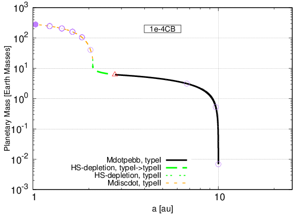
Figure 3 shows that in our approach, the horseshoe gas mass decay is due to the planetary gas accretion and gravitational pushing of the protoplanet. The final planetary gas mass by the time of the horseshoe depletion corresponds to the initial gas mass in the horseshoe region. Thus our simple approach of horseshoe gas accretion is mass conservative.
3.2 Consequences on planet formation
Using the previous outlined modifications, we plot the growth track of a planet starting at au and Myr as a purple line in Figure 1. For the nominal viscosity reported in this work (0.005), the discussed new prescription of gas accretion appears irrelevant, especially in slowing the overall migrating distance to the star. We attribute this result to the faster type II migration rates due to the high -viscosity. In addition, the high -viscosity means high pebble scale height, therefore the pebbles are not in the efficient accretion zones of the planetary embryo. Therefore migration wins over growth, with the planet starting to carve a gap when the cores is approaching 1 au from the star and migrates even further inwards before transitioning fully into slower type II regime. We test the importance of core location in the disc by implanting cores at 20 au in Figure 4. As expected the core now starts carving gap just outside of 2 au but the planets still migrate all the way to the disc’s inner edge. We therefore conclude that, within the framework of the simple power law disc model we used, the difference between NN and CB in slowing inward migration is not very significant for higher viscosity.
Assuming a lower -viscosity (0.0001) in the disc, we clearly see differences appearing between NN and CB model in Figure 1. Both 1e-4NN and the 1e-4CB simulations now accrete pebbles in the efficient 2D regime. This allows the early formation of a gap, before the planet is driven to the inner edge of the disc. The 1e-4CB curve (short dashed purple) starts to diverge relative to the 1e-4NN model (short dashed blue curve), when the planet starts its runaway gas accretion. From this point on, the growth is faster in the 1e-4CB case, because gas accretion is not limited by the disc accretion as long as the horseshoe region is not empty. As soon as the horseshoe region empties, the growth slows down and becomes limited by what the disc can provide. At the same time the planet transitions into Type II migration. Therefore, the intermediate phase between Type I and Type II migration is very short. At the end of the disc lifetime the planet following the 1e-4CB track ends just outside 1 au and with a mass of around 300 Earth masses. For these particular growth tracks (Figure 1), an important difference between 1e-4NN and 1e-4CB is noted in the final planetary orbital positions, but only a small difference is seen in terms of the final planetary mass. Comparing Figure 1 and Figure 4, we note that the difference between NN and CB prescriptions scales with: (i) viscosity and (ii) injection positions of planetary embryos in the discs. The effect of the CB prescription is clearly highlighted for cores implanted in the outer disc. In this prescription the gas surface density of the protoplanetary disc plays a crucial role in the final mass of the planet, as it determines how much material the


planet can accrete from its horseshoe region33 3 The amount of materials in the core’s horseshoe region depends on the accretional viscosity and the core’s location in the disc.. This is a clear difference with respect to the NN model, where the final planetary mass depends only on the mass accretion rate through the disc and not on the total gas surface density. Planets that formed earlier, when the disc is more massive, can grow larger than planets formed later. In addition, if planets are formed late, the differences between CB and NN should be very small due to the limited material available in the horseshoe region (see the global maps (Figures 2, 6 & 7) for more illustration). The corresponding global map for NN and CB models are shown in the first column of the top and the bottom panel of Figure 2, respectively. We see that there are many more super Jupiters in hot/warm orbits with respect to the nominal case (first column of the top panel of Figure 2), because the more rapid transition to Type II migration reduces the overall migration of the planet towards the star. The planets, moreover, are a bit more massive than in the nominal case.
We show in Figure 5 the overall sequence of major events in the track 1e-4CB (short-dashed purple curve) of Figure 1. It is clear from Figure 5 that the planetary migration rate occurs in three regimes (marked by different colors). The type I migration rate scales linearly with planetary mass until it opens a gap. The planet then gradually transitions into the constant slower type II migration rate. We remind the reader that the onset of our horseshoe gas mass depletion corresponds to the intermediate type I/type II regime. In addition, our effective gap parameter profile (black curve) follows the horseshoe gas mass profile (green curve) and is only marginally determined by the gravitational gap opening, highlighting the role of gas accretion for gap opening.
We stress that the formula of Crida & Morbidelli 2007 for the gap depth would predict the opening of a gap with 50% depth at Earth masses, determining the end of pure Type I migration. However, such a gap would cause the blockage of the flux of pebbles at the outer edge of the gap. In other words, opening a gap at 5 Earth masses is inconsistent with estimate of the pebble isolation mass at Earth masses at disc location with (Bitsch et al. 2018). We think that the Crida & Morbidelli 2007 formula, calibrated for giant planets in viscous discs, is not quantitatively reliable for small planets in disc of vanishing viscosity, as stated in Bitsch et al. 2018. Instead, the pebble isolation mass criterion has been investigated in the proper regime by recent hydrodynamical simulations (Lambrechts & Johansen 2014; Bitsch et al. 2018; Ataiee et al. 2018). Thus, we assume that Type I migration operates until the pebble isolation mass.
In the transition period between Type I and Type II migration, the planet implanted at 10 au and at 0.1 Myr in a disc with using the CB accretion prescription (short dashed-purple line in Figure 1) achieves 90 % orbital decay. Applying the dynamic co-rotation torque, we obtain the tracks depicted by the long dashed curves in Figure 1. Following the purple long dashed curve (1e-4CBDyn track) in Figure 1, Type I migration now brings the planet to au.


Runaway gas accretion therefore starts just before 0.4 Myr, when the planet is still beyond 4 au, bringing the planet into the Type II migration regime. Then, as expected, due to the low viscosity of the disc, the migration is slow. In the subsequent 2.6 Myr the planet moves radially by au, finding itself at Earth masses just inside of 3 au at the end of the disc’s lifetime. This result confirms the relevance of the dynamical torque in planet formation.
4 When are the CB accretion and the dynamical torques relevant in planet formation?
The previous section showed that, in the CB prescription and accounting for the dynamical corotation torque, the viscosity of the disc and the location and time of injection of the planetary seed in the disc play a major role. In this section, we show when and where the CB prescription and the dynamical torque become important in planet formation using a global evolution map of planet formation like those of Figure 2. We start by exploring the impact of viscosity in the disc on the global planet formation map. The viscosity in our model controls the migration and accretion speed, for example at a higher viscosity, inward migration is fast and the gas accretion rate of a planet exceeding the pebble isolation mass is high. In addition a lower viscosity reduces the pebble scale height, allowing faster growth during the pebble accretion stage.
It is clear from the simulations with that the lower migration speeds and faster pebble-accretion rates allow the formation of gas giants also in the inner parts of the protoplanetary disc (see the first column plots in Figure 6). On the contrary, for higher viscosity, the gas giant planets have to start forming in the disc outskirts due to the fast inward migration speed that outperforms growth rates (see the first column plots in Figure 2).
The effects of the CB prescription become enhanced at low viscosities. This results in earlier gap opening, less inward migration and slightly larger gas giants (e.g. Figure 1 and Figure 4). However, in the case of , the gas accretion rate in itself is very low, resulting in planets that barely reach super Jupiter mass, indicating that a higher viscosity might be needed to explain very massive giant planets. In addition the effects of the CB prescription depends on the injection time of the planetary embryo. In particular, an early injection time of the planetary embryo results in a stronger effect of the CB accretion compared to later planetary embryo injection times. This is caused due to the fact that the mass of gas in the planet’s horseshoe region is larger at earlier times.
We show in Figure 6 (second column plots) the influence of the dynamical torque on the final masses and positions of planets formed in our model. Quite clearly, the dynamical torque becomes more efficient in slowing-down migration if the disc’s viscosity is smaller (Paardekooper 2014). At high viscosities, the dynamical torque only affects planetary embryos growing initially in the very outer regions of the disc. Cores forming in the inner region (a5 au) of the disc are only barely affected. At low viscosites, the effect of the dynamical torque increases significantly. At , if the dynamical torque is not accounted for, early forming planets have to originate outside of 30 au to stay exterior of 5 au, while planets can form as close as 15 au if the effects of the dynamical torque is included.
We show in Figure 7 the result of planet formation simulations using for discs with higher aspect ratio (). The higher aspect ratio of the disc reduce the pebble accretion rates due to the higher scale height. The high aspect ratio also results in a higher pebble isolation mass resulting in larger planetary cores. This shortens the envelope contraction phase resulting in higher planetary masses, if the planets reach the pebble isolation mass and transition into gas accretion.
Our simulation results hold no surprise in this case, as a higher aspect ratio clearly results in higher planetary masses and at the same time also in faster inward migration. In addition it seems that the effects of the dynamical torque are less enhanced, because for a given planet mass the width of the horseshoe region decreases with increasing disc’s aspect ratio.
Our results indicate that the effects of the CB accretion mechanism and the dynamical torque greatly reduce inward migration in low viscosity environments. As such these effects are important for future planet formation simulations.
5 Conclusion
In this paper we have revisited the work of Bitsch et al. 2015b and Ndugu et al. 2018 on the accretion and migration of planets in a simple approach where pebble accretion is modeled with a constant Stokes number of 0.1. Bitsch et al. 2015b concluded that giant planets that are at a few au from the central star at the end of the disc’s lifetime must have started forming beyond 20 au. This conclusion appears inconsistent with the expectation that the most favorable place for the accretion of a giant planet’s core should be the water ice line, which is probably not beyond au in young protoplanetary discs (Savvidou et al. 2020). This large-scale inward migration is driven by the high viscosity of the disc assumed in Bitsch et al. 2015b, leading to fast inward migration also in the type II regime.
An obvious solution to reduce inward migration, is the reduction of the disc’s viscosity. For low mid viscosity, we have shown that the planet covers a smaller radial distance in type-II migration, as shown also by previous studies. In the case of low viscosities, the entropy driven corotation torque is fully saturated (Paardekooper et al. 2011, e.g.), preventing outward migration. Instead the low viscosity allows a transition into the slower type II migration at lower planetary masses. The low viscosity of the disc limits also the gas accretion rate onto the planet, resulting in lower mass planets in discs with lower viscosity.
Our simulations show that the dynamical torque (Paardekooper 2014) reduces the inward migration before the planet opens a deep gap in the disc. Furthermore, we find that accreting material directly from the horseshoe region (Crida & Bitsch 2017) can help in opening a deep gap, allowing an earlier transition into type II migration and retaining the planet at larger distances from the star.
As already shown by Paardekooper 2014, a viscosity of below a few times is needed for the dynamical torque to operate and slow down migration effectively. If the dynamical torque is as efficient as shown in our work, it could allow giant planets to form close to the water ice line and remain in the outer disc. We thus conclude that the incorporation of the dynamical torques and the accretion from the horseshoe region can have significant influence on the resulting planet population and should be taken into account in future comprehensive planet population synthesis simulation.
Acknowledgments
N.N acknowledge financial support from the International Science Program (ISP) and the Poincaré junior fellowship. E.J appreciate the financial support from the International Science Program (ISP). B.B, thanks the European Research Council (ERC Starting Grant 757448-PAMDORA) for their financial support. We thank an anonymous referee whose comments helped to improve this manuscript.
Data Availability
The codes used to obtain the results in this paper is available upon reasonable request.
Appendix A Implementation of dynamical corotation torque
As hinted in subsection 2.2, the dynamical corotation torque can effectively, reduce type I migration rates in shallow discs with low disc viscosities. Due to this torque, the type I migration rate of a planet is divided by a factor (Paardekooper 2014, Equation 19 in). Therefore, the new type I migration, in the limit of vanishing viscosity, becomes:
| (26) |
where is the classical type I migration rate.
is the mass that the horseshoe region would have had if it had the unperturbed local density of the gas ; and are computed as described in the subsection 3.1. The factor is typically larger than 1, which results in reduced migration. In fact, when the planet has not yet opened a gap by accretion and gravitational pushing , one has:
| (27) | |||||
where is the current location of the planet and is the location where the planet migrated from. The term is smaller than 1 if the planet is migrating inward () and the gradient of the surface density of the disc is smaller than . Thus the term , reducing the inward migration rate.
Appendix B Influence of Stokes number


In protoplanetary discs, the small micrometer dust grains can grow to form larger particles by coagulation (Brauer et al. 2008, e.g.) or condensation (Ros & Johansen 2013, e.g). These growth processes result in different Stokes numbers of particles, which are probably also not uniform in the disc. This has important consequences for the solid accretion rates via pebble accretion. For a fixed pebble surface density, larger Stokes number should lead to faster growth. However, in our model, the pebble surface density increases with reduction in Stokes number (Equation 4) for a fixed pebble flux. Therefore from Equation 5, cores accrete pebbles at a rate proportional to , leading to faster growth with lower Stokes numbers.
We show the impact of different Stokes numbers in our model in Figure 8. Our results clearly indicate that planets growing in environments with larger/small Stokes numbers grow slower/faster and thus smaller/bigger. This can be clearly seen in Figure 8, where the simulations with lower Stokes numbers produce relatively massive giant planets compared to the simulations with larger Stokes numbers. On the other hand, it seems that the influence of Stokes number on the final position of the formed gas giants is not that pronounced at the inner parts of the disc (Figure 8).
We therefore conclude that the Stokes number has an important influence on the outcome of our simulations. However, the effects discussed in the main paper, namely the influence of the CB accretion mechanism and of the dynamical torques are untouched by the difference in Stokes number. In future simulations that aim to reproduce all planet populations from different Stokes numbers should be taken into account.
References
- Ali-Dib (2017) Ali-Dib M., 2017, MNRAS, 467, 2845
- Alibert et al. (2005) Alibert Y., Mousis O., Mordasini C., Benz W., 2005, ApJ, 626, L57
- Alibert et al. (2011) Alibert Y., Mordasini C., Benz W., 2011, A&A, 526, A63
- Andrews et al. (2012) Andrews S. M., et al., 2012, ApJ, 744, 162
- Ataiee et al. (2018) Ataiee S., Baruteau C., Alibert Y., Benz W., 2018, A&A, 615, A110
- Baruteau et al. (2014) Baruteau C., et al., 2014, Protostars and Planets VI, pp 667–689
- Baumann & Bitsch (2020) Baumann T., Bitsch B., 2020, arXiv e-prints, p. arXiv:2004.00874
- Benítez-Llambay et al. (2015) Benítez-Llambay P., Masset F., Koenigsberger G., Szulágyi J., 2015, Nature, 520, 63
- Bergez-Casalou et al. (2020) Bergez-Casalou C., Bitsch B., Pierens A., Crida A., Raymond S. N., 2020, arXiv e-prints, p. arXiv:2010.00485
- Bitsch & Johansen (2017) Bitsch B., Johansen A., 2017, in Pessah M., Gressel O., eds, Astrophysics and Space Science Library Vol. 445, Astrophysics and Space Science Library. p. 339, doi:10.1007/978-3-319-60609-5_12
- Bitsch et al. (2014) Bitsch B., Morbidelli A., Lega E., Crida A., 2014, A&A, 564, A135
- Bitsch et al. (2015a) Bitsch B., Johansen A., Lambrechts M., Morbidelli A., 2015a, A&A, 575, A28
- Bitsch et al. (2015b) Bitsch B., Lambrechts M., Johansen A., 2015b, A&A, 582, A112
- Bitsch et al. (2018) Bitsch B., Morbidelli A., Johansen A., Lega E., Lambrechts M., Crida A., 2018, A&A, 612, A30
- Bottke et al. (2005) Bottke W. F., Durda D. D., Nesvorný D., Jedicke R., Morbidelli A., Vokrouhlický D., Levison H., 2005, Icarus, 175, 111
- Brauer et al. (2008) Brauer F., Dullemond C. P., Henning T., 2008, A&A, 480, 859
- Brügger et al. (2018) Brügger N., Alibert Y., Ataiee S., Benz W., 2018, A&A, 619, A174
- Cassan et al. (2012) Cassan A., et al., 2012, Nature, 481, 167
- Chambers (2018) Chambers J., 2018, ApJ, 865, 30
- Chiang & Goldreich (1997) Chiang E. I., Goldreich P., 1997, ApJ, 490, 368
- Crida & Bitsch (2017) Crida A., Bitsch B., 2017, Icarus, 285, 145
- Crida & Morbidelli (2007) Crida A., Morbidelli A., 2007, MNRAS, 377, 1324
- Crida et al. (2006) Crida A., Morbidelli A., Masset F., 2006, Icarus, 181, 587
- Cridland et al. (2019) Cridland A. J., Eistrup C., van Dishoeck E. F., 2019, A&A, 627, A127
- Dittkrist et al. (2014) Dittkrist K.-M., Mordasini C., Klahr H., Alibert Y., Henning T., 2014, A&A, 567, A121
- Drążkowska & Alibert (2017) Drążkowska J., Alibert Y., 2017, A&A, 608, A92
- Fischer & Valenti (2005) Fischer D. A., Valenti J., 2005, ApJ, 622, 1102
- Flock et al. (2019) Flock M., Turner N. J., Mulders G. D., Hasegawa Y., Nelson R. P., Bitsch B., 2019, A&A, 630, A147
- Fortier et al. (2013) Fortier A., Alibert Y., Carron F., Benz W., Dittkrist K. M., 2013, A&A, 549, A44
- Fressin et al. (2013) Fressin F., et al., 2013, ApJ, 766, 81
- Haisch et al. (2001) Haisch Karl E. J., Lada E. A., Lada C. J., 2001, ApJ, 553, L153
- Hartmann et al. (1998) Hartmann L., Calvet N., Gullbring E., D’Alessio P., 1998, ApJ, 495, 385
- Howard et al. (2010) Howard A. W., et al., 2010, Science, 330, 653
- Ida & Guillot (2016) Ida S., Guillot T., 2016, A&A, 596, L3
- Ida & Lin (2004) Ida S., Lin D. N. C., 2004, ApJ, 604, 388
- Ida & Lin (2008a) Ida S., Lin D. N. C., 2008a, ApJ, 673, 487
- Ida & Lin (2008b) Ida S., Lin D. N. C., 2008b, ApJ, 685, 584
- Ida et al. (2013) Ida S., Lin D. N. C., Nagasawa M., 2013, ApJ, 775, 42
- Ida et al. (2018) Ida S., Tanaka H., Johansen A., Kanagawa K. D., Tanigawa T., 2018, ApJ, 864, 77
- Ikoma et al. (2000) Ikoma M., Nakazawa K., Emori H., 2000, ApJ, 537, 1013
- Johansen & Bitsch (2019) Johansen A., Bitsch B., 2019, arXiv e-prints, p. arXiv:1909.10429
- Johansen & Lacerda (2010) Johansen A., Lacerda P., 2010, MNRAS, 404, 475
- Johansen et al. (2019) Johansen A., Ida S., Brasser R., 2019, A&A, 622, A202
- Johnson et al. (2010) Johnson J. A., Aller K. M., Howard A. W., Crepp J. R., 2010, PASP, 122, 905
- Kanagawa et al. (2018) Kanagawa K. D., Tanaka H., Szuszkiewicz E., 2018, ApJ, 861, 140
- Lambrechts & Johansen (2012) Lambrechts M., Johansen A., 2012, A&A, 544, A32
- Lambrechts & Johansen (2014) Lambrechts M., Johansen A., 2014, A&A, 572, A107
- Lambrechts et al. (2014) Lambrechts M., Johansen A., Morbidelli A., 2014, A&A, 572, A35
- Laughlin & Adams (1997) Laughlin G., Adams F. C., 1997, ApJ, 491, L51
- Levison et al. (2010) Levison H. F., Thommes E., Duncan M. J., 2010, AJ, 139, 1297
- Lin & Ida (1997) Lin D. N. C., Ida S., 1997, ApJ, 477, 781
- Lin & Papaloizou (1986) Lin D. N. C., Papaloizou J., 1986, ApJ, 307, 395
- Lubow & D’Angelo (2006) Lubow S. H., D’Angelo G., 2006, ApJ, 641, 526
- Lynden-Bell & Pringle (1974) Lynden-Bell D., Pringle J. E., 1974, MNRAS, 168, 603
- Machida et al. (2010) Machida M. N., Kokubo E., Inutsuka S.-I., Matsumoto T., 2010, MNRAS, 405, 1227
- Manara et al. (2012) Manara C. F., Robberto M., Da Rio N., Lodato G., Hillenbrand L. A., Stassun K. G., Soderblom D. R., 2012, ApJ, 755, 154
- Masset et al. (2006) Masset F. S., Morbidelli A., Crida A., Ferreira J., 2006, ApJ, 642, 478
- Mayor et al. (1995) Mayor M., et al., 1995, IAU Circ., 6251, 1
- McNeil et al. (2005) McNeil D., Duncan M., Levison H. F., 2005, AJ, 130, 2884
- Miguel et al. (2011) Miguel Y., Guilera O. M., Brunini A., 2011, MNRAS, 412, 2113
- Morales et al. (2019) Morales J. C., et al., 2019, arXiv e-prints, p. arXiv:1909.12174
- Morbidelli (2015) Morbidelli A., 2015, European Planetary Science Congress 2015, held 27 September - 2 October, 2015 in Nantes, France, Online at http://meetingorganizer.copernicus.org/EPSC2015, id.EPSC2015-30, 10, EPSC2015
- Morbidelli et al. (2009) Morbidelli A., Bottke W. F., Nesvorný D., Levison H. F., 2009, Icarus, 204, 558
- Mordasini et al. (2009) Mordasini C., Alibert Y., Benz W., 2009, A&A, 501, 1139
- Mordasini et al. (2015) Mordasini C., Mollière P., Dittkrist K. M., Jin S., Alibert Y., 2015, International Journal of Astrobiology, 14, 201
- Movshovitz & Podolak (2008) Movshovitz N., Podolak M., 2008, Icarus, 194, 368
- Nayakshin (2015) Nayakshin S., 2015, MNRAS, 454, 64
- Ndugu et al. (2018) Ndugu N., Bitsch B., Jurua E., 2018, MNRAS, 474, 886
- Ndugu et al. (2019) Ndugu N., Bitsch B., Jurua E., 2019, MNRAS, 488, 3625
- Nelson et al. (2000) Nelson R. P., Papaloizou J. C. B., Masset F., Kley W., 2000, MNRAS, 318, 18
- Nelson et al. (2013) Nelson R. P., Gressel O., Umurhan O. M., 2013, MNRAS, 435, 2610
- Ogihara et al. (2015) Ogihara M., Morbidelli A., Guillot T., 2015, A&A, 578, A36
- Ormel & Klahr (2010) Ormel C. W., Klahr H. H., 2010, A&A, 520, A43
- Paardekooper (2014) Paardekooper S.-J., 2014, MNRAS, 444, 2031
- Paardekooper et al. (2011) Paardekooper S.-J., Baruteau C., Kley W., 2011, MNRAS, 410, 293
- Piso & Youdin (2014) Piso A.-M. A., Youdin A. N., 2014, ApJ, 786, 21
- Pollack et al. (1996) Pollack J. B., Hubickyj O., Bodenheimer P., Lissauer J. J., Podolak M., Greenzweig Y., 1996, Icarus, 124, 62
- Ronco et al. (2017) Ronco M. P., Guilera O. M., de Elía G. C., 2017, MNRAS, 471, 2753
- Ros & Johansen (2013) Ros K., Johansen A., 2013, A&A, 552, A137
- Santos et al. (2004) Santos N. C., Mayor M., Naef D., Pepe F., Queloz D., Udry S., 2004, in Dupree A. K., Benz A. O., eds, IAU Symposium Vol. 219, Stars as Suns : Activity, Evolution and Planets. p. 311
- Savvidou et al. (2020) Savvidou S., Bitsch B., Lambrechts M., 2020, arXiv e-prints, p. arXiv:2005.14097
- Schoonenberg & Ormel (2017) Schoonenberg D., Ormel C. W., 2017, preprint, (arXiv:1702.02151)
- Shakura & Sunyaev (1973) Shakura N. I., Sunyaev R. A., 1973, A&A, 24, 337
- Singer et al. (2019) Singer K. N., et al., 2019, Science, 363, 955
- Stoll & Kley (2014) Stoll M. H. R., Kley W., 2014, A&A, 572, A77
- Suzuki et al. (2016) Suzuki D., et al., 2016, ApJ, 833, 145
- Tanaka & Ida (1999) Tanaka H., Ida S., 1999, Icarus, 139, 350
- Thommes et al. (2003) Thommes E. W., Duncan M. J., Levison H. F., 2003, Icarus, 161, 431
- Turner et al. (2014) Turner N. J., Fromang S., Gammie C., Klahr H., Lesur G., Wardle M., Bai X.-N., 2014, Protostars and Planets VI, pp 411–432
- Walsh et al. (2011) Walsh K. J., Morbidelli A., Raymond S. N., O’Brien D. P., Mandell A. M., 2011, Nature, 475, 206