Spin superfluidity in noncollinear antiferromagnets

Spintronics has been extremely successful in combining advanced theoretical concepts with practical applications and experiment [1]. Materials with antiferromagnetic ordering are a focus of active research in spintronics due to many desirable properties such as spin dynamics in terahertz range [2], the absence of stray fields, and insensitivity to the presence of magnetic fields [3]. In addition, antiferromagnetic insulators are characterized by long spin diffusion length associated with transport of magnons, making them particularly suitable for spintronics applications such as low dissipation electronic devices [4].

Magnetic insulators can also transport spins in a regime in which the transport can be describe as spin superfluidity [5; 6]. In easy-plane magnets, the spin is then transported over large distances by the coherent order parameter precession [7; 8; 9]. The power-law decay of spin current can enable spin transport over longer distances compared to the diffusive regime [10; 7; 11; 8; 12; 9; 13; 14; 15]. Nevertheless, in ferromagnets the dipole interaction can limit the range of spin superfluid transport [9]. On the other hand, collinear antiferromagnetic insulators could provide a viable platform for realizing the spin superfluidity [8; 16; 17] as demonstrated in experiments on Cr₂O₃ [14] and antiferromagnetic $\nu=0$ quantum Hall state of graphene [15].

Noncollinear antiferromagnets (nAFM) are yet another viable platform for realizing spin flows [18; 19; 20]. The noncollinear conducting magnets can exhibit a multitude of phenomena associated with topology of electronic bands [21], e.g., Mn₃X (X = Ge, Sn, Ga, Ir, Rh, or Pt) magnets exhibit the anomalous [22] and spin [23] Hall responses. Various magnon-mediated responses relying on magnon spin-momentum locking, topology of magnonic bands, and coupling to phonons have been studied theoretically, promising observation of spin related phenomena in insulating antiferromagnets [24; 25; 26; 27; 28; 29; 30; 31; 32].

In this work, we analytically study viability of spin superfluid transport in insulating nAFM. In general, the U(1) symmetry of magnetic ordering can be hampered by various anisotropies. The highly symmetric hexagonal environment considered in this work can be beneficial for realizing spin superfluid transport. Hexagonal nAFM can exhibit relevant phenomena, e.g., the appearance of domain walls [33; 34] and Goldstone modes [35]. Furthermore, spin superfluid transport has been studied numerically in a triangular nAFM [36]. In this work, we offer analytical results with a detailed discussion of the generalized spin-mixing conductance and spin current injection into nAFM. We identify the power-law decay feature of the spin superfluid transport in a nonlocal experimental setup. Our simple results can help in designing and interpreting experiments on spin superfluidity in nAFM.

Long-wavelength Hamiltonian— In nAFM, the exchange interaction is often dominant, which approximately endows the system with an $SO(3)$ symmetry given that all other interactions, e.g., anisotropy, DMI, are very weak. We start with constructing a long-wavelength $SO(3)$ field theory to describe the nAFMs and regard other weak terms as additional perturbations. In a two-dimensional nAFM with three sublattices (e.g., kagome, triangular), the exchange interactions favor fully compensated spin configurations, which in the presence of other interactions may acquire a very small net magnetization. Therefore, we parametrize the spins $\bm{S}_{i}$ of length $S$ in each triangular plaquette as [37]

where $\bm{n}_{i}$ ($i=1,2,3$) sets a reference ordered state allowed by exchange interactions with

$\hat{R}\in SO(3)$ is a rotation matrix which generates degenerate states by acting on the reference state; $\bm{L}$ describes small deviation from the compensated spin structure with the magnitude $L\ll 1$. $\hat{R}$ and $\bm{L}$ together generate all possible spin configurations on three sublattices. To the leading order in $\bm{L}$, $\bm{S}_{i}=S\hat{R}[\bm{n}_{i}+\bm{L}-\bm{n}_{i}(\bm{L}\cdot\bm{n}_{i})]$, and the net angular momentum density,

where $s=S\hbar/A_{\text{uc}}$, $T_{ab}=\delta_{ab}-\frac{1}{3}\sum_{i}n_{i}^{a}n^{b}_{i}$, and $A_{\text{uc}}$ is the area of a unit cell.

With the forgoing parametrization, the system is generally described by a Lagrangian [37],

where $(\Omega_{t})_{i}=-\frac{1}{2}R_{i\alpha}\epsilon_{\alpha\beta\gamma}(\hat{R}^{T}\partial_{t}\hat{R})_{\beta\gamma}$. Here, the first term is derived from the spin kinetic energy; the second term originates from the exchange interaction, e.g., for the nearest exchange $J$, we obtain $\varrho\propto\hbar^{2}/(JA_{\text{uc}})$; the last term describes the second-order gradient expansion of exchange coupling with tensor $\hat{P}_{ij}$ encoding the exchange interactions and lattice geometry. From the Euler-Lagrange equation [33], we obtain:

from which the field $\bm{m}$ can be removed from Eq. (4), i.e.,

This is the so-called nonlinear $\sigma$ model [37; 38].

To determine the tensor $\hat{P}_{ij}$ for a hexagonal-symmetry lattice, kagome or triangular, when exchange is the dominant interaction, we explore the spin wave behavior by following Ref. [35]. We consider small fluctuations upon the reference state by using $\hat{R}=\exp[-i\bm{\theta}\cdot\hat{\bm{\mathcal{J}}}]$, where $(\mathcal{J}_{i})_{jk}=-i\epsilon_{ijk}$ with $\epsilon_{ijk}$ being the Levi-Civita tensor and a vector $\bm{\theta}$ describes the small deviation with $|\bm{\theta}|\ll 1$. The spin-wave energy is obtained from the leading-order expansion of the second term in Eq. (6),

Due to the highly symmetric hexagonal environment, $\theta_{z}$ acts as a scalar and $\theta_{x},\theta_{y}$ act as two components of a vector under symmetry transformations. Using the symmetry constraints, we recover the form of $\hat{P}_{ij}$ tensor:

where the arbitrary coefficients $\kappa$, $\eta$, $\lambda$, and $\mu$ scale as the exchange strength $J$. For triangular and kagome lattices with the nearest exchange interaction, their values are summarized in Table. 1.

From Eq. (6), the spin-wave Lagrangian reads $\mathcal{L}=(\varrho/2)(\dot{\bm{\theta}})^{2}-\mathcal{U}$. By using Eq. (Spin superfluidity in noncollinear antiferromagnets), we can obtain three linearly dispersive Goldstone modes [35] $\omega_{i}=v_{i}k$ with $v_{1}=\sqrt{2(2\eta+\lambda+\mu)/\varrho}$, $v_{2}=\sqrt{2(\kappa+\eta+\lambda+\mu)/\varrho}$, $v_{3}=\sqrt{2(\kappa+\eta)/\varrho}$. Here, $\omega_{1}$ corresponds to the scalar mode $\theta_{z}$, and $\omega_{2,3}$ comes from the vector modes $\theta_{x},\theta_{y}$ [35].

DMI and anisotropy— In nAFMs, the field theory used to describe exchange interactions should be modified by the aforementioned weak interactions that remove the $SO(3)$ symmetry and gap out the Goldstone modes. To take these interactions into account in centrosymmetric crystals, we first consider their microscopic expressions.

In a kagome lattice (see Fig. 1), we consider the DMI term, e.g. typical to jarosites [39],

where $\bm{D}_{ij}=D_{z}\hat{\bm{z}}+\bm{D}_{\parallel}$, $\bm{D}_{\parallel}=D_{p}\hat{\bm{n}}_{ij}$ with $\hat{\bm{n}}_{12}=(\frac{\sqrt{3}}{2},-\frac{1}{2},0)$, $\hat{\bm{n}}_{23}=(0,1,0)$, and $\hat{\bm{n}}_{31}=(-\frac{\sqrt{3}}{2},-\frac{1}{2},0)$. We first consider DMI to the leading-order in spatial gradients and obtain the energy density,

where $(\hat{X}_{k})_{ab}=\sum_{i,j=1}^{3}S^{2}\mathcal{D}^{k}_{ij}n_{i}^{a}n_{j}^{b}$ and $\mathcal{D}^{k}_{ij}=D^{k}_{ij}/A_{\text{uc}}$. By using Eq. (10) and the representation of the rotation matrix, $\hat{R}=\exp[-i\bm{\theta}\cdot\hat{\bm{\mathcal{J}}}]\exp[-i\phi\hat{\mathcal{J}}_{z}]$, the leading correction of the DMI term is obtained by expanding Eq. (10) to the lowest order of $\theta_{i}$ ($i=x,y,z$),

where $\Delta=-3\sqrt{3}\mathcal{D}_{z}S^{2}>0$. The out-of-plane DMI suppresses spin rotations other than those with respect to $z$-axis, reducing the SO(3) symmetry to a $U(1)$ rotation symmetry. Furthermore, the DMI in Eq. (9) constrains the ground state of the system and gaps out the Goldstone modes $\omega_{i}=\sqrt{v_{i}^{2}k^{2}+\Delta/\varrho}$ for $i=2,3$, while the $\omega_{1}$ mode is intact.

To capture a small gap in the $\omega_{1}$ mode, we expand Eq. (1) to the first order in $\bm{L}$ and substitute it in Eq. (9). The contribution proportional to $\bm{m}$ can be written in a compact form,

where $\bm{\mathcal{B}}$ is a “magnetic field”:

with $(Z_{kl})_{ab}=(S/6\hbar)\sum_{i,j}\sum_{c}D_{ij}^{k}(n^{a}_{i}\delta^{bc}-n_{i}^{a}n_{j}^{b}n_{j}^{c}+\delta^{ac}n_{j}^{b}-n_{i}^{a}n_{j}^{b}n_{i}^{c})(\hat{T}^{-1}\hat{R}^{T})_{cl}$. Combing this term with Eqs. (4) and (10) and eliminating $\bm{m}$, the effective Lagrangian becomes:

where $\mathcal{U}[\hat{R}]=\text{tr}[\hat{P}_{ij}\partial_{i}\hat{R}^{T}\partial_{j}\hat{R}]+\mathcal{H}_{D}$. The $\bm{\mathcal{B}}$ term breaks the rotation symmetry and gaps out the $\omega_{1}$ mode.

In a triangular lattice (see Fig. 1), the intrinsic DMI is forbidden by the lattice symmetry, while the ground state can be stabilized by the energy density,

where $\mathcal{K}=K/A_{\text{uc}}$, $\mathcal{K}_{z}=K_{z}/A_{\text{uc}}$, with $K,K_{z}$ being the easy-axis and easy-plane anisotropy constants, respectively. By substituting $\bm{S}_{i}\approx\hat{R}\bm{n}_{i}$ in Eq (15), the anisotropy term gives a correction,

where $\Delta=3(\mathcal{K}_{z}+\mathcal{K})S^{2}$. When $\mathcal{K}\ll\mathcal{K}_{z}$, we can approximately neglect the easy-axis term, and thus the system approximately respects $U(1)$ symmetry. The Goldstone modes, $\omega_{2,3}$, acquire a gap, $\sqrt{\Delta/\varrho}$. A small gap in the $\omega_{1}$ mode is described by $\mathcal{K}$.

Spin superfluidity— In the following, we focus on the spin transport facilitated by approximate $U(1)$ symmetry. We assume that the system is driven by a weak perturbation when compared to the gap of the $\omega_{2}$ and $\omega_{3}$ modes, while large enough to overcome the barrier corresponding to the gap of the $\omega_{1}$ mode. By adding $\mathcal{H}_{A}$ or $\mathcal{H}_{D}$ to the Lagrangian (6) and neglecting the hard modes, the Lagrangian of the soft mode becomes:

where $\mathcal{A}=2(2\eta+\lambda+\mu)$. On the other hand, the third component of Eq. (5) is reduced to $m_{z}\approx\varrho\partial_{t}\phi$. Therefore, we arrive at a continuity equation,

where a spin current density with polarization along $z$-axis can be identified as

The spin superfluidity in nAFM will be affected by dissipation effects. Within the Lagrangian formalism, we can add dissipation using the Rayleigh dissipation function [40]:

where $\hat{Q}$ is a symmetric matrix with non-negative eigenvalues [41; 42]. From symmetry considerations applied to three equivalent sublattices, we obtain that $Q_{ij}=r_{1}$ for $i=j$ and $Q_{ij}=r_{2}$ for $i\neq j$ where $r_{1}$ and $r_{2}$ are real parameters. The Rayleigh function can be approximately written as $\mathcal{R}=\text{tr}[\hat{\mathcal{Q}}\partial_{t}\hat{R}^{T}\partial_{t}\hat{R}]$ with $\mathcal{Q}_{ab}=\frac{1}{2}\sum_{ij}Q_{ij}n_{i}^{a}n_{j}^{b}$ to describe dissipation of the soft mode, i.e.,

where $\alpha=3(r_{1}+2r_{2})/s$ is a dimensionless dissipation parameter.

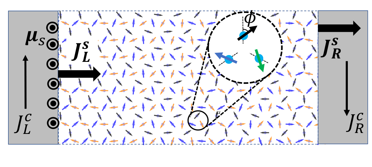
To activate spin dynamics in a magnetic insulator, a spin Hall current can be induced in a neighbouring normal metal layer (see Fig. 2). A build-up of spin accumulation in a normal metal will then lead to injection of spin current into the magnetic insulator layer. The boundary condition on the interface can be derived via the magnetoelectronic circuit theory [43; 44; 45; 46; 47]. When exchange interactions dominate, the spin injection and pumping together give the total spin current across the interface (see details in Supplemental Material):

where $\bm{\omega}$ is the instantaneous angular velocity for slow dynamics of the order parameter and $\hat{\mathcal{G}}^{m}$ is the generalized spin-mixing conductance tensor [47]. Under assumption of $C_{3}$ symmetry (or axial symmetry with respect to $\bm{l}$ axis), the tensor $\hat{\mathcal{G}}^{m}$ takes the following form:

where ${\cal G}^{\uparrow\downarrow}_{r(i)}=\sum_{mn}\operatorname{Re}(\operatorname{Im})(\delta_{nm}-r_{mn}^{\uparrow\uparrow}r_{mn}^{\downarrow\downarrow*})$, ${\cal G}_{\parallel}=\sum_{mn}(|r_{mn}^{\uparrow\downarrow}|^{2}+|r_{mn}^{\downarrow\uparrow}|^{2})$, and $\bm{l}$ is the unit vector normal to the plane spanned by three-sublattice spins (cf. Eq. (59) in Ref. [47]). Here, $r^{\sigma\sigma^{\prime}}_{mn}$ stands for reflection amplitudes for electrons reflected from channel $n$ into channel $m$ in the normal metal and $\bm{l}$ is the quantization axis for $\sigma,\sigma^{\prime}=\uparrow,\downarrow$.

By writing the Euler-Lagrange equation with Rayleigh dissipation for Eqs. (17) and (21), the dynamic equation for $\phi$ reads,

We use a steady-state ansatz [7; 8], $\phi(x,t)=\varphi(x)+\Omega t$, where $\Omega$ is a constant frequency. For almost in-plane spin order, the angular velocity is $\bm{\omega}\approx\dot{\phi}\hat{z}$ and $\bm{l}=\hat{z}$. We also assume spin accumulation along $z$-direction, $\bm{\mu}_{s}=\mu\hat{z}$. Equations (19), (22), and (Spin superfluidity in noncollinear antiferromagnets) then lead to the boundary conditions on the left ($x=0$) and right ($x=L$) interfaces:

where $g_{a}=\mathcal{G}_{\parallel,a}/\mathcal{V}$ ($a=L,R$) with $\mathcal{V}$ being the area of interface. Combining the boundary condition and the steady-state ansatz, we obtain,

where $g_{\alpha}=4\pi\alpha sL/\hbar$.

Above approximations need to be revisited when weak in-plane DMI or easy-axis anisotropy are present. We obtain a Lagrangian describing the soft mode:

where $c_{s}=\sqrt{\mathcal{A}/\varrho}$ and $m_{s}$ is the mass term due to weak in-plane DMI or easy-axis anisotropy. To activate spin transport, the gradient needs to overcome the barrier induced by the gap, i.e., $|\nabla\phi|\geq m_{s}/c_{s}$. The spiral-like phase supporting spin superfluid will become energetically unstable when the field $\phi$ varies faster than $1/\xi$ where $\xi=\sqrt{\varrho c_{s}^{2}/\Delta}$ is the characteristic length associated with the gap of $\omega_{2}$ and $\omega_{3}$ modes, i.e., $|\nabla\phi|\leq\xi^{-1}$. Thus, the spin-superfluid transport is only possible under the assumption,

We first discuss the kagome lattice nAFM with in-plane DMI in which case $m_{s}=\sqrt{3/2}D_{p}S/\hbar$. As estimated in Table. 2, we find that different iron jarosites fulfil criteria (28) very well and hence are very promising for experimental realization of spin superfluidity. In a triangular lattice, the easy-axis anisotropy hinders ideal spin superfluidity leading to the last term in Eq. (27) with $m_{s}=3S\sqrt{KJ}/\hbar$. Equation (28) leads to the condition $\sqrt{K/K_{z}}\ll 1$.

The spin-superfluid transport can be measured in a nonlocal setup in Fig. 2 [48]. The spin Hall current builds up an effective spin accumulation, $\mu_{s}=(4\pi/g_{L})J_{\text{SH}}^{s}$, where $J_{\text{SH}}^{s}=\vartheta_{\text{SH}}(\hbar/2e)J^{c}_{L}$ is the spin current induced by the charge current $J^{c}_{L}$, and $\vartheta_{\text{SH}}$ is the spin Hall angle in the leads [49; 48; 50]. The spin current mediated by the collective dynamics of nAFM passes across the second interface by virtue of the spin pumping effect, and it is converted into a charge current in the right lead, $J^{c}_{R}=(\vartheta_{\text{SH}}\sigma/d)(\hbar/2e)\Omega$, where $\sigma$ and $d$ are, respectively, the conductivity and thickness of the right metal layer. The nonlocal transport is characterized by a drag coefficient, $\mathcal{D}=J_{R}^{c}/J^{c}_{L}=\mathcal{D}_{0}/(1+L/L_{\alpha})$, where $\mathcal{D}_{0}=\pi\vartheta_{\text{SH}}^{2}\sigma\hbar/(2e^{2}gd)$, $g=g_{L}=g_{R}$, and $L_{\alpha}=\hbar g/(2\pi\alpha s)$. Assuming $\vartheta_{\text{SH}}=0.1$, $\sigma=0.1\,\mu\Omega^{-1}\cdot\text{cm}^{-1}$, $d=1\text{nm}$, $g\sim 10^{19}\text{m}^{-2}$, $\alpha=10^{-3}$, $s\sim\hbar/a^{3}$, and a lattice constant $a\sim 1\text{nm}$, we obtain $\mathcal{D}_{0}\sim 0.1$ and $L_{\alpha}\sim 1\mu\text{m}$. These results are similar to collinear systems [7; 8] and show that the long crossover length $L_{\alpha}$ can be used as a key signature of spin superfluidity.

Conclusions— We have used an $SO(3)$-invariant field theory to describe three-sublattice antiferromagnets with hexagonal lattice in an exchange interaction dominated limit. When weak interactions, such as DMI or anisotropy, are added, the symmetry is approximately reduced to $U(1)$. We have shown that in this limit, three-sublattice antiferromagnets can facilitate a spin superfluid transport. Using generalized spin-mixing conductance, we have also described the injection of spin current and its power-law decay in a nonlocal experimental setup. Our results indicate that the magnitude of spin current is constrained by parasitic DMI or anisotropies, which can help in finding suitable materials. In particular, we estimate that iron jarosites can be promising for realizing spin superfluidity in noncollinear antiferromagnets. Noncollinear antiferromagnets hold promise for realizing spin flows with low dissipation and the theoretical framework presented here can be useful for exploring the interplay between transport phenomena [53; 54] and topological defects, i.e., domain walls [33; 34], or skyrmions [55].

This work was supported by the U.S. Department of Energy, Office of Science, Basic Energy Sciences, under Award No. DE-SC0021019.

Supplemental Material

References

- Tsymbal and Žutić [2019] E. Y. Tsymbal and I. Žutić, eds., Spintronics Handbook: Spin Transport and Magnetism (CRC Press, Taylor & Francis Group, Boca Raton, 2019).
- Olejník et al. [2018] K. Olejník, T. Seifert, Z. Kašpar, V. Novák, P. Wadley, R. P. Campion, M. Baumgartner, P. Gambardella, P. Němec, J. Wunderlich, et al., Sci. Adv. 4, eaar3566 (2018).
- Baltz et al. [2018] V. Baltz, A. Manchon, M. Tsoi, T. Moriyama, T. Ono, and Y. Tserkovnyak, Rev. Mod. Phys. 90, 015005 (2018).
- Lebrun et al. [2018] R. Lebrun, A. Ross, S. A. Bender, A. Qaiumzadeh, L. Baldrati, J. Cramer, A. Brataas, R. A. Duine, and M. Kläui, Nature 561, 222 (2018).
- Sonin [2010] E. Sonin, Adv. Phys. 59, 181 (2010).
- Halperin and Hohenberg [1969] B. I. Halperin and P. C. Hohenberg, Phys. Rev. 188, 898 (1969).
- Takei and Tserkovnyak [2014] S. Takei and Y. Tserkovnyak, Phys. Rev. Lett. 112, 227201 (2014).
- Takei et al. [2014] S. Takei, B. I. Halperin, A. Yacoby, and Y. Tserkovnyak, Phys. Rev. B 90, 094408 (2014).
- Skarsvåg et al. [2015] H. Skarsvåg, C. Holmqvist, and A. Brataas, Phys. Rev. Lett. 115, 237201 (2015).
- König et al. [2001] J. König, M. C. Bønsager, and A. H. MacDonald, Phys. Rev. Lett. 87, 187202 (2001).
- Sonin [2017] E. B. Sonin, Phys. Rev. B 95, 144432 (2017).
- Flebus et al. [2016] B. Flebus, S. A. Bender, Y. Tserkovnyak, and R. A. Duine, Phys. Rev. Lett. 116, 117201 (2016).
- Iacocca et al. [2017] E. Iacocca, T. J. Silva, and M. A. Hoefer, Phys. Rev. B 96, 134434 (2017).
- Yuan et al. [2018] W. Yuan, Q. Zhu, T. Su, Y. Yao, W. Xing, Y. Chen, Y. Ma, X. Lin, J. Shi, R. Shindou, et al., Sci. Adv. 4, eaat1098 (2018).
- Stepanov et al. [2018] P. Stepanov, S. Che, D. Shcherbakov, J. Yang, R. Chen, K. Thilahar, G. Voigt, M. W. Bockrath, D. Smirnov, K. Watanabe, et al., Nat. Phys. 14, 907 (2018).
- Qaiumzadeh et al. [2017] A. Qaiumzadeh, H. Skarsvåg, C. Holmqvist, and A. Brataas, Phys. Rev. Lett. 118, 137201 (2017).
- Takei et al. [2016] S. Takei, A. Yacoby, B. I. Halperin, and Y. Tserkovnyak, Phys. Rev. Lett. 116, 216801 (2016).
- Mook et al. [2019a] A. Mook, R. R. Neumann, J. Henk, and I. Mertig, Phys. Rev. B 100, 100401 (2019a).
- Flebus et al. [2019] B. Flebus, Y. Tserkovnyak, and G. A. Fiete, Phys. Rev. B 99, 224410 (2019).
- Ma et al. [2020] B. Ma, B. Flebus, and G. A. Fiete, Phys. Rev. B 101, 035104 (2020).
- Šmejkal et al. [2018] L. Šmejkal, Y. Mokrousov, B. Yan, and A. H. MacDonald, Nat. Phys. 14, 242 (2018).
- Chen et al. [2014] H. Chen, Q. Niu, and A. H. MacDonald, Phys. Rev. Lett. 112, 017205 (2014).
- Železný et al. [2017] J. Železný, Y. Zhang, C. Felser, and B. Yan, Phys. Rev. Lett. 119, 187204 (2017).
- Owerre [2017] S. A. Owerre, Phys. Rev. B 95, 014422 (2017).
- Laurell and Fiete [2018] P. Laurell and G. A. Fiete, Phys. Rev. B 98, 094419 (2018).
- Mook et al. [2019b] A. Mook, J. Henk, and I. Mertig, Phys. Rev. B 99, 014427 (2019b).
- Kim et al. [2019] K.-S. Kim, K. H. Lee, S. B. Chung, and J.-G. Park, Phys. Rev. B 100, 064412 (2019).
- Okuma [2017] N. Okuma, Phys. Rev. Lett. 119, 107205 (2017).
- Li et al. [2020a] B. Li, A. Mook, A. Raeliarijaona, and A. A. Kovalev, Phys. Rev. B 101, 024427 (2020a).
- Li et al. [2020b] B. Li, S. Sandhoefner, and A. A. Kovalev, Phys. Rev. Research 2, 013079 (2020b).
- Park et al. [2020] S. Park, N. Nagaosa, and B.-J. Yang, Nano Letters 20, 2741 (2020).
- Go et al. [2019] G. Go, S. K. Kim, and K.-J. Lee, Phys. Rev. Lett. 123, 237207 (2019).
- Ulloa and Nunez [2016] C. Ulloa and A. S. Nunez, Phys. Rev. B 93, 134429 (2016).
- Yamane et al. [2019] Y. Yamane, O. Gomonay, and J. Sinova, Phys. Rev. B 100, 054415 (2019).
- Dasgupta and Tchernyshyov [2020] S. Dasgupta and O. Tchernyshyov, arXiv:2004.02790 (2020).
- Goli and Manchon [2020] V. M. L. D. P. Goli and A. Manchon, arXiv:2005.13481 (2020).
- Dombre and Read [1989] T. Dombre and N. Read, Phys. Rev. B 39, 6797 (1989).
- Azaria et al. [1992] P. Azaria, B. Delamotte, and D. Mouhanna, Phys. Rev. Lett. 68, 1762 (1992).
- Elhajal et al. [2002] M. Elhajal, B. Canals, and C. Lacroix, Phys. Rev. B 66, 014422 (2002).
- Gilbert [2004] T. Gilbert, IEEE Trans. Magn. 40, 3443 (2004).
- Yuan et al. [2019] H. Y. Yuan, Q. Liu, K. Xia, Z. Yuan, and X. R. Wang, Europhys. Lett. 126, 67006 (2019).
- Kamra et al. [2018] A. Kamra, R. E. Troncoso, W. Belzig, and A. Brataas, Phys. Rev. B 98, 184402 (2018).
- Brataas et al. [2000] A. Brataas, Y. V. Nazarov, and G. E. W. Bauer, Phys. Rev. Lett. 84, 2481 (2000).
- Brataas et al. [2006] A. Brataas, G. E. Bauer, and P. J. Kelly, Phys. Rep. 427, 157 (2006).
- Belashchenko et al. [2016] K. D. Belashchenko, A. A. Kovalev, and M. van Schilfgaarde, Phys. Rev. Lett. 117, 207204 (2016).
- Tserkovnyak and Ochoa [2017] Y. Tserkovnyak and H. Ochoa, Phys. Rev. B 96, 100402 (2017).
- Flores et al. [2020] G. G. B. Flores, A. A. Kovalev, M. van Schilfgaarde, and K. D. Belashchenko, Phys. Rev. B 101, 224405 (2020).
- Tserkovnyak and Bender [2014] Y. Tserkovnyak and S. A. Bender, Phys. Rev. B 90, 014428 (2014).
- Tserkovnyak et al. [2005] Y. Tserkovnyak, A. Brataas, G. E. W. Bauer, and B. I. Halperin, Rev. Mod. Phys. 77, 1375 (2005).
- Ochoa et al. [2018] H. Ochoa, R. Zarzuela, and Y. Tserkovnyak, Phys. Rev. B 98, 054424 (2018).
- Matan et al. [2006] K. Matan, D. Grohol, D. G. Nocera, T. Yildirim, A. B. Harris, S. H. Lee, S. E. Nagler, and Y. S. Lee, Phys. Rev. Lett. 96, 247201 (2006).
- Matan et al. [2011] K. Matan, B. M. Bartlett, J. S. Helton, V. Sikolenko, S. Mat’aš, K. Prokeš, Y. Chen, J. W. Lynn, D. Grohol, T. J. Sato, et al., Phys. Rev. B 83, 214406 (2011).
- Kim et al. [2015] S. K. Kim, S. Takei, and Y. Tserkovnyak, Phys. Rev. B 92, 220409 (2015).
- Zou et al. [2019] J. Zou, S. K. Kim, and Y. Tserkovnyak, Phys. Rev. B 99, 180402 (2019).
- Rosales et al. [2015] H. D. Rosales, D. C. Cabra, and P. Pujol, Phys. Rev. B 92, 214439 (2015).
- Tserkovnyak et al. [2002] Y. Tserkovnyak, A. Brataas, and G. E. W. Bauer, Phys. Rev. B 66, 224403 (2002).
- Brouwer [1998] P. W. Brouwer, Phys. Rev. B 58, R10135 (1998).
- Brataas et al. [2012] A. Brataas, Y. Tserkovnyak, G. Bauer, and P. Kelly, Spin pumping and spin transfer (Oxford University Press, United Kingdom, 2012), pp. 87–135.