Further Development of iCIPT2 for Strongly Correlated Electrons

As pointed out recentlyLiu 2020; Liu 2020, among the three components of electronic structure theory (i.e., relativity, correlation, and QED), it is correlation that is most challenging, especially for strongly correlated systems. Roughly speaking, a strongly correlated system features multiple open-shell orbitals or nearly degenerate electronic states thanks to the existence of a dense set of energetically adjacent frontier orbitals, such that there does not exist a single, leading component in the wave functions. Because of this, single-reference methods are bound to fail, especially for those low-spin states. Instead, multi-reference methodsChaudhuri et al. 2005; Hoffmann et al. 2009; Lyakh et al. 2012; Sherrill and Schaefer III 1999; Szalay et al. 2012; Lischka et al. 2018 are needed even for a qualitative description of such states. A unanimous assumption underlying standard multi-reference methods is that the full many-electron Hilbert space can be decomposed into a model space $P$ and the remaining complement $Q=1-P$, which are responsible for the static and dynamic components of the overall correlation, respectively. Then, according to when the static and dynamic correlations are handled, such methods can be classified into three families, viz. “static-then-dynamic”, “dynamic-then-static”, and “static-dynamic-static” (SDS)Liu and Hoffmann 2016. Given their great success in investigating low-lying electronic states of many chemical systems, it must be realized that such multi-reference methods still have strong limitations. For instances, it is by no means trivial to maintain the same model space, so as to produce smooth potential energy surfaces. Even if this can be achieved, there is no guarantee that the chosen model space is equally good for all geometries and all target states. Even more seriously, those states that have little projections in the chosen model space cannot well be described. Taking all these facts into account, one can classify chemical systems into weakly correlated (which can well be described by single-reference methods), moderately correlated (which can well be described by standard multi-reference methods with a moderate model space, typically much smaller than the complete active space (CAS) of 18 electrons in 18 orbitals), and strongly correlated (which require a large model space and are therefore beyond the capability of standard multi-reference methods). As a matter of fact, the concept of model space looses its original meaning for the so-defined strongly correlated systems because the states in a large model space $P$ and those formally in the orthogonal complement $Q$ are heavily intersected in both energy and composition. In other words, the static and dynamic correlations are in such cases strongly entangled and interchangeable. Moreover, solving the large-model-space problem itself is already a heavy task, needless to say the subsequent treatment of dynamic correlation (NB: the larger the model space, the larger the first-order interacting space (FOIS)). So the question is how to design an adaptive method that can adapt to the variable static correlation automatically and can meanwhile handle the residual dynamic correlation efficiently. It appears that the most promising way to this end is to introduce some selection procedure, so as to build up progressively a compact yet accurate variational space $P$, in full accordance with the nature of the system under concern. In this spirit, a number of near-exact approaches have been designed in the past, including density matrix renormalization group (DMRG)White 1992; White 1993; White and Martin 1999; Mitrushenkov et al. 2001; Chan and Head-Gordon 2002; Chan and Sharma 2011; Sharma and Chan 2012; Wouters and Van Neck 2014; Olivares-Amaya et al. 2015; Li and Chan 2017; Baiardi and Reiher 2020, full configuration interaction (FCI) quantum Monte Carlo (FCIQMC)Booth et al. 2009; Cleland et al. 2010; Blunt et al. 2017; Petruzielo et al. 2012; Holmes et al. 2016; Ten-no 2013; Ghanem et al. 2019; Blunt 2019; Dobrautz et al. 2019; Neufeld and Thom 2020, cluster-analysis-driven FCIQMCDeustua et al. 2018, adaptive coupled-cluster (CC)Lyakh and Bartlett 2010, full CC reductionXu et al. 2018; Xu et al. 2020, deterministically projected FCIZhang and Evangelista 2016, many-body expanded FCIEriksen et al. 2017; Eriksen and Gauss 2018; Eriksen and Gauss 2019; Eriksen and Gauss 2019, incremental FCIZimmerman 2017; Zimmerman 2017, rank-reduction FCIFales et al. 2018, fast randomized interaction-based FCIGreene et al. 2019, intrinsic scaling-based correlation expansionBytautas and Ruedenberg 2004; Bytautas and Ruedenberg 2004, as well as selected CI (sCI) Greer 1998; Coe and Paterson 2012; Ohtsuka and Hasegawa 2017; Coe 2018; Holmes et al. 2016; Garniron et al. 2017; Holmes et al. 2017; Sharma et al. 2017; Chien et al. 2018; Yao et al. 2020; Evangelista 2014; Schriber and Evangelista 2016; Schriber and Evangelista 2017; Schriber et al. 2018; Tubman et al. 2016; Lehtola et al. 2017; Tubman et al. 2020; Tubman et al. 2018; Liu and Hoffmann 2014; Liu and Hoffmann 2016; Lei et al. 2017; Zhang et al. 2020; Garniron et al. 2018; Wang et al. 2019; Giner et al. 2016; Scemama et al. 2018. Among these, the sCI type of approaches, which are largely a revival of the very old ideasBender and Davidson 1969; Whitten and Hackmeyer 1969; Huron et al. 1973; Evangelisti et al. 1983; Buenker and Peyerimhoff 1974 in one way or another, are the simplest in structure and rival those more sophisticated approaches as shown in a recent blind testEriksen et al. 2020. As the newest member of the sCI family, the iCIPT2 approachZhang et al. 2020 proposed by the present authors, i.e., the combination of iterative CI (iCI)Liu and Hoffmann 2016 with selection and second-order perturbation theory (PT2) has a number of salient features:

1. (1)

   Born from the restricted SDS frameworkLiu and Hoffmann 2014 for strongly correlated electrons, iCILiu and Hoffmann 2016 is a parameter-free, exact solver of the FCI eigenvalue problem. It constructs and diagonalizes a very small Hamiltonian matrix $\bar{\mathbf{H}}$ (see Sec. 2) at each macro/micro-iteration but can converge quickly to the exact solutions. The major bottleneck of iCI lies therefore only in the construction of the Hamiltonian matrix $\mathbf{H}$ in the basis of Slater determinants (SD) or configuration state functions (CSF) before contracted to $\bar{\mathbf{H}}$ for diagonalization. Since $\mathbf{H}$ is extremely sparse, the combination of iCI with selection is a natural choice, leading to “selected iCI” (SiCI) as an near-exact solver of FCI. To be more practical, the (one-step) SiCI can be performed in two steps, with the first step accounting for the static correlation whereas the second step for a second-order perturbative treatment of the dynamic correlation. This can be achieved by a single parameter $C_{min}$, which controls the size of the variational space and hence the final accuracy. This scheme has been dubbed as iCIPT2Zhang et al. 2020.

2. (2)

   The selection is carried out over the entire Hilbert space or a very large active space (which can in this context be viewed as a coarse-grained selection step). Those unimportant doubly excited orbital configurations (CFG) are first screened out based on the upper bounds of the elements of $\mathbf{H}$. After this integral-driven screening, the individual CSFs of a selected CFG are further selected using their approximate first-order coefficients. In short, although the selection is performed on individual CSFs, it is CFGs that are used as the organizing units. Given a coefficient pruning-threshold $C_{min}$, the selection of important CFGs/CSFs is performed iteratively until convergence.

3. (3)

   At each iteration for the growth of wave function, the FOIS is decomposed into disjoint subspaces, so as to reduce memory requirement on one hand and facilitate parallelization on the other.

4. (4)

   A new technique called TUGA (tabulated unitary group approach) is introduced to compute and reuse the basic coupling coefficients (BCC), i.e., the matrix elements of $U(n)$ generators over CSF pairs.

5. (5)

   Because of the use of CSFs as the many-electron basis, full spin symmetry is always maintained, which is of vital importance for describing low-spin states of general open-shell systems as well as subsequent perturbative treatment of spin-orbit couplings.

6. (6)

   Upon termination of the selection, dynamic correlation is estimated by using the state-specific Epstein-Nesbet type of second-order perturbation theory (ENPT2).

7. (7)

   The linear relationship between the total versus second-order correlation energies allows for an accurate extrapolation.

The present contribution amounts to further enhancing the efficiency of iCIPT2 by using (a) a new ranking criterion for the selection of CFGs/CSFs (see Sec. 4), (b) a new particle-hole algorithm for the construction and update of $\mathbf{H}$ in the variational space (see Sec. 5), and (c) the Timsort algorithmTim; Tim for sorting the joint variational and first-order interacting spaces (see Sec. 6). Before these, we ought to outline the SDS family of methods in Sec. 2 and the essentials of TUGA in Sec. 3. A close comparison of TUGA with Table-CIBuenker 1980; Buenker 1986; Krebs and Buenker 1995; Khait and Hoffmann is also given in the latter, since they are both configuration-driven alogithms. The chromium dimer and an iron-sulfur cluster, $\text{[}\text{Fe}{\vphantom{\text{X}}}_{\vphantom{\text{2}}\smash[t]{\text{2}}}^{\vphantom{\smash[t]{\text{2}}}\hphantom{\text{2}}\text{}}\text{S}{\vphantom{\text{X}}}_{\vphantom{\text{2}}\smash[t]{\text{2}}}^{\vphantom{\smash[t]{\text{2}}}\hphantom{\text{2}}\text{}}\text{(}\text{SCH}{\vphantom{\text{X}}}_{\vphantom{\text{2}}\smash[t]{\text{3}}}^{\vphantom{\smash[t]{\text{2}}}\hphantom{\text{3}}\text{}}\text{)}\text{]}\text{}{\vphantom{\text{X}}}_{\vphantom{\text{2}}\smash[t]{\text{4}}}^{\vphantom{\smash[t]{\text{2}}}\hphantom{\text{4}}\text{}}$^2-, are finally taken as examples to reveal the efficacy of the improved implementation of iCIPT2 (see Sec. 7). The presentation is closed with concluding remarks in Sec. 8.

The restricted “static-dynamic-static” (SDS) frameworkLiu and Hoffmann 2014 for strongly correlated electrons gives rise first to the SDSCI approach, which is a minimal MRCI with the following form for the wave function $|\Psi_{i}\rangle$ of state $i\in[1,N_{P}]$,

	$\displaystyle|\Psi_{i}\rangle$	$\displaystyle=\sum_{k=1}^{mN_{P}}|\tilde{\Phi}_{k}\rangle C_{k,i},\quad m=3\mbox{ or }4,$		(1)
	$\displaystyle|\tilde{\Phi}_{k}\rangle$	$\displaystyle=|\Psi_{k}^{(0)}\rangle=\sum_{|J\nu\rangle\in P}|J\nu\rangle\bar{C}_{\nu,k}^{J(0)},\quad k\in[1,N_{P}],$		(2)
	$\displaystyle|\tilde{\Phi}_{k+N_{P}}\rangle$	$\displaystyle=|\Psi_{k}^{(1)}\rangle=Q\frac{1}{E_{k}^{(0)}-H_{0}}QH|\Psi_{k}^{(0)}\rangle=\sum_{|J\nu\rangle\in Q}|J\nu\rangle\bar{C}_{\nu,k}^{J(1)},\quad k\in[1,N_{P}],$		(3)
	$\displaystyle|\tilde{\Phi}_{k+2N_{P}}\rangle$	$\displaystyle=P_{\mathrm{s}}|\Theta_{k}\rangle,\quad k\in[1,N_{P}],$		(4)
	$\displaystyle|\tilde{\Phi}_{k+3N_{P}}\rangle$	$\displaystyle=P_{\mathrm{s}}|\Theta_{k}^{\prime}\rangle,\quad k\in[1,N_{P}]\quad(\mbox{ if }m>3),$		(5)
	$\displaystyle P$	$\displaystyle=\sum_{J\nu}^{d_{R}}|J\nu\rangle\langle J\nu|=P_{\mathrm{m}}+P_{\mathrm{s}},\quad P_{\mathrm{m}}=\sum_{k=1}^{N_{P}}|\Psi_{k}^{(0)}\rangle\langle\Psi_{k}^{(0)}|,\quad Q=1-P.$		(6)

Here, the first two sets of $N_{P}$ functions $\{|\tilde{\Phi}_{k}\rangle\}$ are nothing but the zeroth-order (primary) and first-order (external) functions, respectively. To account for changes in the static correlation (described by $\{|\Psi_{k}^{(0)}\rangle\}_{k=1}^{N_{P}}$) due to the presence of dynamic correlation (described by $\{|\Psi_{k}^{(1)}\rangle\}_{k=1}^{N_{P}}$), $N_{P}$ secondary (buffer) functions $\{|\Theta_{k}\rangle\}_{k=1}^{N_{P}}$, Eq. (4), are further introduced, which can be defined in a number ways. For instance, the not-energy-biased Lanczos-type functions (denoted as Buf(1)), $\{H|\Psi_{k}^{(1)}\rangle\}_{k=1}^{N_{P}}$, turn out to be very effectiveLiu and Hoffmann 2014. An alternative choice might be the second set of $N_{P}$ zeroth-order functions $\{|\Psi_{k}^{(0)}\rangle\}_{k=N_{P}+1}^{2N_{P}}$ (denoted as Buf(0)) in the spirit of intermediate Hamiltonian theory, the first set of $N_{P}$ second-order functions $\{|\Psi_{k}^{(2)}\rangle\}_{k=1}^{N_{P}}$) (denoted as Buf(2)) in the spirit of perturbation theory or the $N_{P}$ approximate eigenvectors of the preceding iteration (denoted as Buf(3)) in the spirit of conjugate gradient theoryHuang et al. 2017. While Buf(2) is very expensive, both Buf(0) and Buf(3) are very easy to handle because the Hamiltonian matrix elements can readily be evaluatedHuang et al. 2017. As a matter of fact, Buf(0) and Buf(3) can be applied simultaneously without increasing the computational overhead. In this case, we will have $m=4$ in Eq. (1). Otherwise, we have $m=3$ in Eq. (1) with Buf(1) alone. The yet unknown expansion coefficients are to be determined by the generalized secular equation

$\displaystyle\bar{\mathbf{H}}\mathbf{C}=\mathbf{S}\mathbf{C}\mathbf{E}.$

(7)

Since all the functions $\{|\tilde{\Phi}_{k}\rangle\}_{k=N_{P}+1}^{mN_{P}}$ are fully contracted (i.e., linear combinations of the CSFs $\{|\nu\rangle\}$ generated from CFGs $\{|J\rangle\}$) and are specific to the primary state $|\Psi_{k}^{(0)}\rangle$, the dimension of Eq. (7) is just 3 (or 4) times the number ($N_{P}$) of target states, no matter how many electrons and how many orbitals are correlated. Although restricted as such, it has been shownSong et al. that SDSCI is a very effective variational method for both ground and excited states. Two extensions of SDSCI have been considered so far, SDSPT2Liu and Hoffmann 2014; Lei et al. 2017 and iCILiu and Hoffmann 2016, both with Buf(1) alone. The former amounts to replacing the $QHQ$ block of the Hamiltonian matrix in Eq. (7) with $QH_{0}Q$. Different from most variants of multi-reference second-order perturbation theory (MRPT2), the CI-like SDSPT2 treats single and multiple states in the same way and is particularly advantageous when a number of states are nearly degenerate, thanks to the efficacy of the secondary states in revising the coefficients of the primary states. In contrast, iCI takes the solutions of Eq. (7) as new primary states $\{|\Psi_{k}^{(0)}\rangle\}_{k=1}^{N_{P}}$ and repeats the SDS procedure (1) until convergence. Clearly, each iteration (defined as macro-iteration) accesses a space that is higher by two ranks than that of the preceding iteration. Up to $2i$-tuple excitations (relative to the initial primary space) can be accessed if $i$ macro-iterations are carried out. A few micro-iterations $j$ can be invoked at each macro-iteration so as to relax the contraction coefficients. As such, every iCI($i,j$) corresponds to a physically meaningful model. It has been shown both theoretically and numerically that iCI can converge quickly from above to FCI even when starting with a very poor initial guess. More generally, iCI can be viewed as a particular sequential, exact partial diagonalization of a huge matrix, by getting first the roots of one portion of the matrix and then those of an enlarged portion, until the full matrix, whereas its micro-iterations can be generalized to an iterative vector interaction (iVI) approachHuang et al. 2017 for the roots of a given matrix treated as a whole. Again, each iteration of iVI constructs and diagonalizes a $mN_{P}\times mN_{P}$ matrix ($m=3\mbox{ or }4$) in the form of Eq. (7). In particular, by combining with the energy-vector following technique, iVI can directly access interior roots belonging to a predefined window, without knowing the number and characters of the rootsHuang and Liu 2019.

As stated before, iCIPT2 amounts to splitting iCI into two steps, the first of which accounts for the static correlation by selecting important CFGs/CSFs in an iterative manner, whereas the second of which accounts for the residual dynamic correlation via a second-order perturbation theory. It is the improvement of iCIPT2 that is under concern here.

The very first issue pertinent to iCIPT2 is how to evaluate the Hamiltonian matrix elements over randomly selected CSFs $\{|J\nu\rangle\}$. In this context, the configuration-driven Table-CI approachBuenker 1980; Buenker 1986; Krebs and Buenker 1995; Khait and Hoffmann may be a possible choice. However, it involves line-up permutations of open-shell orbitals, which become ineffective for CFGs of many open-shell orbitals (say, $>10$). To avoid such line-up permutations, we have introduced a “tabulated unitary group approach” (TUGA)Zhang et al. 2020 (originally called “tabulated orbital configuration-based unitary group approach”). Since the UGAPaldus 1974; Paldus and Boyle 1980; Shavitt 1981 is itself rather involved, we here recapitulate the essentials of TUGA. The first step is to break the spin-free, second-quantized Hamiltonian

	$\displaystyle H$	$\displaystyle=$	$\displaystyle\sum_{i,j}h_{ij}E_{ij}+\frac{1}{2}\sum_{i,j,k,l}(ij|kl)e_{ij,kl},$		(8)
	$\displaystyle E_{ij}$	$\displaystyle=$	$\displaystyle\sum_{\sigma}a_{i\sigma}^{\dagger}a_{j\sigma}=E_{ji}^{\dagger},$		(9)
	$\displaystyle e_{ij,kl}$	$\displaystyle=$	$\displaystyle\sum_{\sigma,\tau}a_{i\sigma}^{\dagger}a_{k\tau}^{\dagger}a_{l\tau}a_{j\sigma}=E_{ij}E_{kl}-\delta_{jk}E_{il}=\{E_{ij}E_{kl}\}$		(10)
		$\displaystyle=$	$\displaystyle\{E_{kl}E_{ij}\}=e_{kl,ij}=e^{\dagger}_{ji,lk}$

into a form that is consistent with the diagrams employed in the UGAPaldus and Boyle 1980 for the BCC between CSFs. Specifically,

	$\displaystyle H$	$\displaystyle=$	$\displaystyle H_{1}^{0}+H_{2}^{0}+H_{1}^{1}+H_{2}^{1}+H_{2}^{2},$		(11)
	$\displaystyle H_{1}^{0}$	$\displaystyle=$	$\displaystyle\sum_{i}h_{ii}E_{ii},$		(12)
	$\displaystyle H_{1}^{1}$	$\displaystyle=$	$\displaystyle\sum_{i<j}h_{ij}E_{ij}+\sum_{i>j}h_{ij}E_{ij},$		(13)
	$\displaystyle H_{2}^{0}$	$\displaystyle=$	$\displaystyle\frac{1}{2}\sum_{i}(ii|ii)E_{ii}(E_{ii}-1)+\sum_{i<j}\left[(ii|jj)E_{ii}E_{jj}+(ij|ji)e_{ij,ji}\right],$		(14)
	$\displaystyle H_{2}^{1}$	$\displaystyle=$	$\displaystyle\sum_{i\neq j}\left[(ii|ij)(E_{ii}-1)E_{ij}+(ij|jj)E_{ij}(E_{jj}-1)\right]$		(15)
		$\displaystyle+$	$\displaystyle\sum_{i\neq j\neq k}\left[(ij|kk)E_{ij}E_{kk}+(ik|kj)e_{ik,kj}\right],$
	$\displaystyle H_{2}^{2}$	$\displaystyle=$	$\displaystyle\sum_{i\leq k}\sum_{j\leq l}^{\prime}\left[2^{-\delta_{ik}\delta_{jl}}(ij|kl)e_{ij,kl}+(1-\delta_{ik})(1-\delta_{jl})(il|kj)e_{il,kj}\right],$		(16)

where the superscripts 0, 1, and 2 in $H_{i}$ ($i=1,2$) indicate that the terms contribute to the Hamiltonian matrix elements over two CFGs that are related by zero, single, and double excitations, respectively, whereas the prime in Eq. (16) indicates that $\{j,l\}\cap\{i,k\}=\emptyset$. For two identical CFGs $|I\rangle$, the Hamiltonian matrix elements can be calculated most efficiently asZhang et al. 2020

	$\displaystyle\langle I\mu|H_{1}^{0}+H_{2}^{0}|I\nu\rangle$	$\displaystyle=\delta_{\mu\nu}\{\frac{1}{2}\sum_{i}n_{i}^{R}[h_{ii}+\epsilon_{i}+(n_{i}^{R}-2)g_{ii}]+\sum_{i}\Delta_{i}^{I}[\epsilon_{i}+(n_{i}^{R}-1)g_{ii}]$
		$\displaystyle+\sum_{i\leq j}\Delta_{i}^{I}g_{ij}\Delta_{j}^{I}\}+\sum_{i<j}(ij|ji)\langle I\mu|e_{ij,ji}^{1}|I\nu\rangle\delta(n_{i}^{I},1)\delta(n_{j}^{I},1),$		(17)
	$\displaystyle f_{ij}$	$\displaystyle=h_{ij}+\sum_{k}n_{k}^{R}[(ij|kk)-\frac{1}{2}(ik|kj)],$		(18)
	$\displaystyle\epsilon_{i}$	$\displaystyle=f_{ii}=h_{ii}+\sum_{k}n_{k}^{R}g_{ik},\quad g_{ik}=(ii|kk)-\frac{1}{2}(ik|ki)=g_{ki},$		(19)
	$\displaystyle\Delta_{i}^{I}$	$\displaystyle=n_{i}^{I}-n_{i}^{R},$		(20)

where $\{n_{i}^{R}\}$ are the occupation numbers of the spatial orbitals of a common reference CFG $|R\rangle$ (either Hartree-Fock (HF) or restricted open-shell HF). The superscript 0 or 1 in $e_{ij,kl}$ (see Eq. (17)) refers to the intermediate angular momentum $X$ due to the coupling of two spin-$\frac{1}{2}$ functions. If $|I\rangle=E_{ij}|J\rangle$, the corresponding Hamiltonian matrix elements read (under the Yamanouchi-Kotani (YK) phasePaldus and Boyle 1980)

$$\begin{split}\langle I\mu|H_{1}^{1}+H_{2}^{1}|J\nu\rangle&=\left\langle I\mu|E_{ij}|J\nu\right\rangle\left[f_{ij}+\sum_{k}\Delta_{k}^{J}[(ij|kk)-\frac{1}{2}(ik|kj)]\right.\\ &+\left.\frac{1}{2}n_{i}^{J}(ii|ij)+(\frac{1}{2}n_{j}^{J}-1)(ij|jj)\right]\\ &+\sum_{k\in\mbox{ exterior open}}(ik|kj)\langle I\mu|e_{ik,kj}^{1}|J\nu\rangle\\ &+\sum_{k\in\mbox{ interior open}}(ik|kj)\left[\frac{1}{2}\left\langle I\mu|E_{ij}|J\nu\right\rangle+\langle I\mu|E_{kj}E_{ik}|J\nu\rangle\right],\end{split}$$

(21)

where ‘exterior open’ and ‘interior open’ emphasize that level $k$ belongs to the non-overlapping ($k<\min(i,j)$ or $k>\max(i,j)$) and overlapping ($\min(i,j)<k<\max(i,j)$) cases, respectively, and is singly occupied. On the other hand, if $|I\rangle=e_{ij,kl}|J\rangle$ subject to $\{j,l\}\cap\{i,k\}=\emptyset$, the Hamiltonian matrix elements read

$\displaystyle\langle I\mu|H_{2}^{2}|J\nu\rangle=\left[2^{-\delta_{ik}\delta_{jl}}(ij|kl)\langle I\mu|e_{ij,kl}|J\nu\rangle+(1-\delta_{ik})(1-\delta_{jl})(il|kj)\langle I\mu|e_{il,kj}|J\nu\rangle\right].$

(22)

At this stage two important points can be observed:

1. (1)

   Thanks to the conjugacy (bra-ket inversion) relations $\langle I\mu|E_{ij}|J\nu\rangle=\langle I\mu|E_{ij}|J\nu\rangle^{*}=\langle J\nu|E_{ji}|I\mu\rangle$ and $\langle I\mu|e_{ij,kl}|J\nu\rangle=\langle I\mu|e_{ij,kl}|J\nu\rangle^{*}=\langle J\nu|e_{ji,lk}|I\mu\rangle$ in the absence of spin-orbit couplings, only generators $E_{ij}$ with $i>j$ and $e_{ij,kl}$ with $k\geq i$ and $k>l\geq j$ need to be considered explicitly. They correspond to the s2, c$x$ and d$x$ ($x\in[1,7]$) types of diagrams shown in Figs. 2 and 3 of Ref. 66. More specifically, the s2, c4, c6 and d2 diagrams are required for the evaluation of Eq. (21), while the other c$x$ and d$x$ types of diagrams are needed for the evaluation of Eq. (22). Once such BCCs are available, those conjugate ones can be obtained simply by matrix transpose.

2. (2)

   The BCCs $\langle I\mu|E_{ij}|J\nu\rangle$ and $\langle I\mu|e_{ij,kl}|J\nu\rangle$ depend only on the relative occupations of the CFG pair $(I,J)$ but not on the individual orbitals $\{i,j,k,l\}$. Moreover, the common zero or doubly occupied orbitals need not be considered explicitly because their segment values are just one under the YK phase. Therefore, they can be rewritten as $\langle I\mu|E_{\bar{i}\bar{j}}|J\nu\rangle$ and $\langle I\mu|e_{\bar{i}\bar{j},\bar{k}\bar{l}}|J\nu\rangle$, respectively, in terms of the reduced orbital indices (ROI) $\{\bar{i},\bar{j},\bar{k},\bar{l}\}$ after deleting the common zero or doubly occupied orbitals. Note that the ROIs have one-to-one correspondence with the original orbital indices (see the example in Table 1). This way, the same BCCs can be used for very many integrals sharing the same ROIs.

After deleting the common zero or doubly occupied orbitals in the bra and ket CFGs, we are left with seven occupation patterns, each of which can be assigned a code number as shown in Table 2. Every pair of CFGs can therefore be characterized by a reduced occupation table (ROT) consisting of two sequences, ROT_Orb and ROT_Code. The former records the orbital indices to fetch molecular integrals, whereas the latter records the corresponding code sequence (e.g., (012430) for the example shown in Table 1) to determine the generators, with the following rules: (1) if CFG $|I\rangle$ arises from $|J\rangle$ by exciting one electron from orbital $j$ to orbital $i$, $\bar{j}$ would then correspond to code 2 or 4, while $\bar{i}$ to code 1 or 3 because of the relations $n_{j}^{I}=n_{j}^{J}-1$ and $n_{i}^{I}=n_{i}^{J}+1$. (2) If CFG $|I\rangle$ arises from $|J\rangle$ by exciting two electrons from orbitals $j$ and $l$ $(\geq j)$ to orbitals $i$ and $k$ $(\geq i)$ [NB: $\{i,k\}\cap\{j,l\}=\emptyset$], $\bar{j}$ and $\bar{l}$ $(\geq\bar{j})$ would correspond to code 2, 4 or 6, while $\bar{i}$ and $\bar{k}$ $(\geq\bar{i})$ to code 1, 3 or 5 because of the relations $n_{j}^{I}=n_{j}^{J}-1$, $n_{l}^{I}=n_{l}^{J}-1$, $n_{i}^{I}=n_{i}^{J}+1$ and $n_{k}^{I}=n_{k}^{J}+1$. Codes 6 and 5 further imply $\bar{j}=\bar{l}$ and $\bar{i}=\bar{k}$, respectively. (3) If $\bar{i}<\bar{j}$ in $E_{\bar{i}\bar{j}}$ or $\bar{k}<\bar{l}$ in $e_{\bar{i}\bar{j},\bar{k}\bar{l}}$, a bra-ket inversion should be invoked when calculating the BCCs in terms of the diagrams documented in Table 3. To search and sort the code sequences efficiently, each ROT_Code will be converted to an array of 64-bit integers (3 bits per code). It is clear that, to reutilize the BCCs efficiently, the CFG pairs with the same ROT_Code must be grouped together. Instead of the red-black tree type of bilinear search employed beforeZhang et al. 2020, we adopt here an array-based sorting algorithm: (a) generate all connected CFG pairs and store them in one array; (b) loop over each CFG pair and identify its ROT_Orb and ROT_Code; (c) sort the array based on ROT_Code. This way, those CFG pairs sharing the same ROT_Code (and hence the same BCCs) are adjacent to each other and form a segment in the array. To expedite the sorting process, the code sequences can further be characterized by their lengths and category numbers (CN) defined in Table 3. The latter just number different ranges of the generators ($\mathrm{CN}=0$ for singles and $\mathrm{CN}\in[1,7]$ for doubles) and are hence directly related to the diagrams required for the evaluation of the BCCs. This new sorting algorithm is significantly faster than the red-black trees employed before, although the latter is not really expensive for this purpose.

To be compatible with the desired generator ranges, we have to represent and store properly the CFGs and corresponding CSFs. A CFG can first be represented by an array of occupation numbers, Occ[$i$]=$n_{i}$, $i\in[0,N_{orb}-1]$, with $N_{orb}$ being the total number of spatial orbitals. The comparison of a CFG pair can then be performed efficiently with Algorithm 3 presented previouslyZhang et al. 2020. A CFG pair $(I,J)$ is said to be singly or doubly connected if $|I\rangle$ can be obtained by exciting one or two electrons from $|J\rangle$. CFG $|I\rangle$ is stored preceding CFG $|J\rangle$ (i.e., $I<J$) if and only if $n_{p}^{I}>n_{p}^{J}$ for $p=\max\{x|n_{x}^{I}\neq n_{x}^{J}\}$. A more compact representation of CFGs is to use two bits to store the occupancy number of each spatial orbital. Specifically, $(00)_{2}$, $(01)_{2}$ and $(11)_{2}$ are used for $n_{i}=0$, 1, and 2, respectively. A CFG can then be represented by an array, OrbOccBinary, of 64-bit integers. This representation was used for both bra and ket CFGs in our previous implementation. Now it is discovered that the single occupancy in the bra CFG can be represented by $(10)_{2}$ instead of $(01)_{2}$, so as to make the identification of ROT_Code more efficiently. As can be seen from Table 4, the bitwise XOR operations on the so-defined binary occupation codes (BOC) always give $(00)_{2}$ for common zero or doubly occupied orbitals, such that the identification of ROT_Code can be achieved based fully on bit operations. Such double representation requires $M_{CFG}=2\times 8\left(\lfloor\frac{N_{orb}-1}{32}\rfloor+1\right)$ bytes of memory for storing a CFG.

A CFG $|I\rangle$ can generate $N^{I}_{S,S}$, genealogically coupled CSFs $\{|I\mu\rangle\}_{\mu=0}^{N_{S,S}^{I}-1}$ of total spin $S$, with $N^{I}_{S,S}$ being

$$N_{S,M=S}^{I}=\frac{2S+1}{\frac{1}{2}N_{o}^{I}+S+1}C_{N_{o}^{I}}^{\frac{1}{2}N_{o}^{I}-S},$$

(23)

where $N_{o}^{I}$ is the (seniority) number of open-shell orbitals in CFG $|I\rangle$. Such CSFs are characterized uniquely by the Shavitt step numberShavitt 1977 sequences $\{(d_{0}^{\mu}d_{1}^{\mu}\cdots)\}|_{\mu=0}^{N_{S,S}^{I-1}}$, which can be arranged in a lexical order (i.e., $|I\mu\rangle$ precedes $|I\nu\rangle$ if and only if $d_{p}^{\mu}<d_{p}^{\nu}$ for $p=\min\{x|d_{x}^{\mu}\neq d_{x}^{\nu}\}$), so as to fix the relative ordering $\mu$ uniquely. A 32-bit integer is required to store the relative ordering of CSFs $\{|I\mu\rangle\}$. Since both its BOC and lexical order have to be stored, the memory requirement for storing a CSF is $M_{CFG}+8$ bytes due to memory alignment. The odering of CSFs is defined as follows: if CSF $|I\mu\rangle$ and $|J\nu\rangle$ stem from the same CFG, then $|I\mu\rangle<|J\nu\rangle$ if $\mu<\nu$; otherwise, let $Occ_{Y}$ ($Y=I,J$) be the corresponding occupation array of CFG $|Y\rangle$ and $i=\arg\max_{j}\{Occ_{I}[j]\neq Occ_{J}[j]\}$, then $|I\mu\rangle<|J\nu\rangle$ if $Occ_{I}[i]>Occ_{J}[i]$. In view of Eq. (23), a large number of CSFs can be generated from a CFG of high seniority $N_{o}^{I}$ but only a few of them may contribute discernibly. Therefore, it is absolutely necessary to do individual selections of CSFs.

After the above detailed description of TUGA, a gross comparison with the Table-CI approachBuenker 1980; Buenker 1986; Krebs and Buenker 1995; Khait and Hoffmann is in order. Although both are configuration-driven algorithms for calculating the Hamiltonian matrix elements over randomly selected CSFs, they actually differ significantly. First of all, Table-CI is closely related to the symmetric group approach (SGA)Duch and Karwowski 1985 in view of its explicit tabulation of line-up permutations, whereas TUGA is plainly an implementation of the UGA Paldus 1974; Paldus and Boyle 1980; Shavitt 1981, in terms of the tabulated ROTs rather than the famous graphical representationShavitt 1977; Shavitt 1978 (which is efficient only for well-structured wave functions). Secondly, TUGA and Table-CI differ in the handling of open-shell orbitals. While Table-CI always defines CFGs with doubly occupied orbitals sitting together and open-shell orbitals sitting together (which involves reordering of the orbitals for each CFG), TUGA adopts a universal orbital ordering defined in the very beginning. The common open-shell orbitals are eliminated in Table-CI by virtue of line-up permutations, leaving a relatively small number of unique interaction patterns between SDs resulting from non-identical open-shell orbitals. However, the BCCs between CSFs are dependent on the relative positions of common open-shell orbitals. Therefore, they are not permuted in TUGA but stay where they are after deleting the common zero or doubly occupied orbitals. This increases merely the lengths of code sequences but not the number of ROTs (NB: every CFG pair corresponds to a ROT). In essence, the ROTs in TUGA play the same role in classifying unique interacting CFG pairs at the integral level as the Tables defined in Table-CI. The former are calculated on an as-needed basis, whereas the latter, characterized by a number of parameters (i.e., $\Delta K$, $P$, $Q$, and $R$ determined by the relative occupations of CFG pairs; see Ref. 82 for more details), are created and stored in advance. Thirdly, TUGA evaluates the Hamiltonian matrix elements directly between CSFs, whereas Table-CI has to assemble them via transformations of those between SDs (which can be viewed as an effective means to avoid the overly complicated matrix elements of line-up permutations $Q$ over CSFs, as required by the genuine SGADuch and Karwowski 1985).

In short, TUGA has been based on the single, simple fact that the segment values for common zero or doubly occupied orbitals are always one under the YK phasePaldus and Boyle 1980, such that the BCCs are determined solely by those common open-shell orbitals or orbitals with different occupancy numbers (which are encoded in the code sequences) and can be calculated directly through products of their segment values.

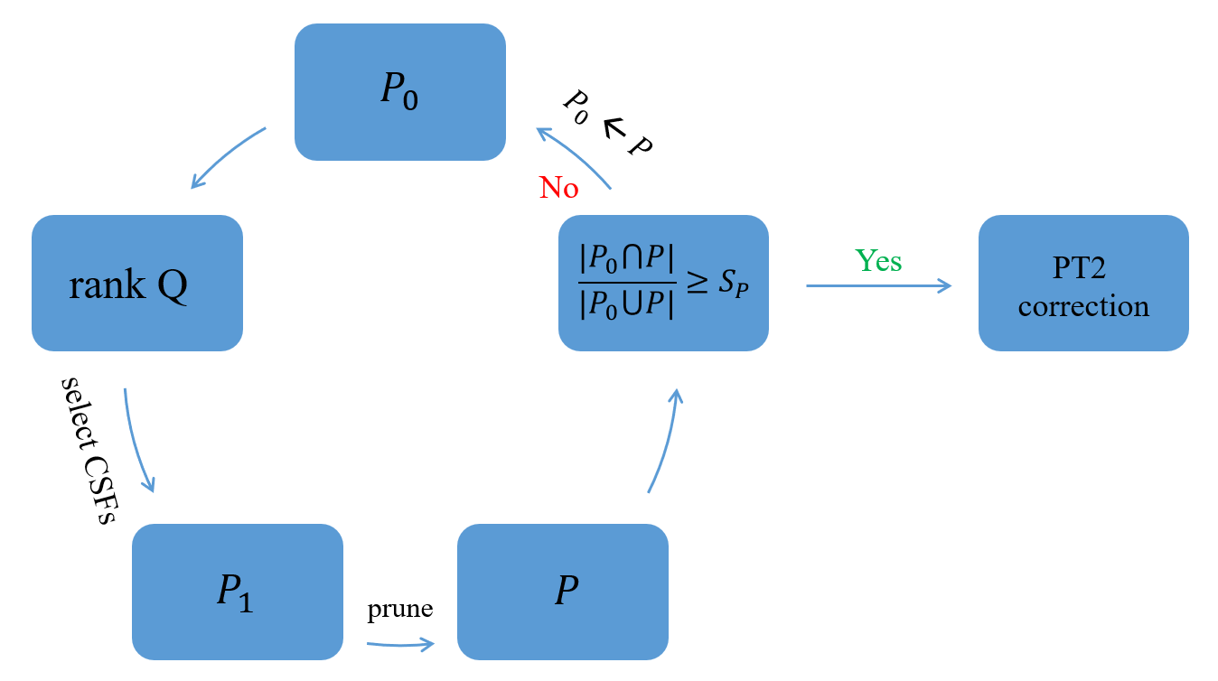
The aim of selection is to find a better variational space $P$ by feeding in a guess space $P_{0}$. This can be achieved in two steps, ranking and pruning. In the ranking step, proper rank values for the CSFs in the FOIS $Q$ $(=1-P_{0})$ will be evaluated. Those CSFs with rank values larger than the given ranking-threshold are put into $P_{0}$, leading to an expanded space $P_{1}$. In the pruning step, the Hamiltonian matrix in $P_{1}$ is first constructed and diagonalized. Those CSFs with coefficients smaller in absolute value than the given pruning-threshold are then discarded, so as to reduce $P_{1}$ to $P$. The procedure is repeated until the energies obtained by diagonalizing $P$ and $P_{0}$ are sufficiently close. Such a two-step selection scheme has been adopted by most sCIs. Yet, a number of refinements has been introduced in our own implementationZhang et al. 2020:

1. (1)

   A combined integral- and coefficient-driven algorithm is used for the selection, viz. prior to the selection of individual CSFs with their (approximate) first-order coefficients as rank values, a integral-driven screening of unimportant, doubly connected CFG pairs is first carried out based on upper bounds $\tilde{H}^{IJ}$ of $\langle I\mu|H_{2}^{2}|J\nu\rangle$ (which are independent of CSFs, see Table 3).

2. (2)

   To minimize the usage of memory, an increment access of the $Q$ space is invoked, with a dynamically adjusted integral-threshold $\varepsilon_{k}$ ($=\frac{1}{2}\varepsilon_{k-1})$. For a given $\varepsilon_{k}$ of iteration $k$ (i.e., $Q[\varepsilon_{k}]$), the selection is repeated until $P[\varepsilon_{k}]$ and $P_{0}[\varepsilon_{k}]$ are sufficiently similar in composition (i.e., $\frac{|P_{0}[\varepsilon_{k}]\bigcap P[\varepsilon_{k}]|}{|P_{0}[\varepsilon_{k}]\bigcup P[\varepsilon_{k}]|}\geq 0.95$).

3. (3)

   Natural orbitals (NO) are also generated dynamically (i.e., for each converged $P[\varepsilon_{k}]$; for more details, see Algorithm 4 in Ref. 66).

4. (4)

   A residue-based algorithmStampfuß and Wenzel 2005; Tubman et al. 2020; Tubman et al. 2018 is used for establishing the connections between randomly selected CFGs and CSFs.

5. (5)

   The diagonalization of Hamiltonian matrix is performed with the iVI-Buf(0+3) approachHuang et al. 2017; Huang and Liu 2019, which has the potential to access directly the roots of a given energy window.

6. (6)

   The size of the resulting variational space $P[\varepsilon_{k}=0]$ is controlled by a single parameter $C_{min}$ (coefficient pruning-threshold), for other parameters have been fixed to conservative values.

It has been demonstrated that the above selection can generate a very compact yet accurate variational space. However, its efficiency is not yet satisfactory because of the following reasons related to the first four points above: (a) the adopted ranking criterion is too good (and hence expensive) for the purpose of selection. (b) Although the incremental access of the $Q$ space is very effective in reducing memory requirement and does not affect the final result, it does result in additional iterations and hence slow down the selection procedure. (c) The generation of NOs and hence transformation of integrals are performed too many times, which is unnecessary. (d) The residue-based algorithm is not optimal for identifying the connections between the CFGs in $P$. In particular, it does not allow for an easy construction of the Hamiltonian matrix in CSR format. To resolve these issues, we here introduce a simpler ranking criterion, remove the incremental access of $Q$, simplify the generation of NO, and replace the residue-based algorithm with a particle-hole algorithm for Hamiltonian construction (see Sec. 5).

In view of many-body perturbation theory (MBPT), the most rigorous ranking of a CSF $|I\mu\rangle\in Q$ is its first-order coefficient in absolute value

$$f(|I\mu\rangle,C_{min})=\left|\frac{\sum_{|J\nu\rangle\in P_{0}}H^{IJ}_{\mu\nu}C^{J}_{\nu}}{E_{0}-H_{\mu\mu}^{II}}\right|\geq C_{min},\quad H^{IJ}_{\mu\nu}=\langle I\mu|H|J\nu\rangle,$$

(24)

which is to be called ‘CIPSI criterion’, with CIPSI standing for ‘configuration interaction with perturbative selection made iteratively’Huron et al. 1973. If those $|J\nu\rangle\in P_{0}$ with small coefficients are excluded from the sum in the numerator of Eq. (24), it may be termed ‘pruned CIPSI criterion’ or simply ‘ASCI criterion’, as adopted by adaptive sampling CITubman et al. 2016. Noticing that the computational expense of Eq. (24) results from both the sum in the numerator and the evaluation of the denominator, a dramatically simplified criterion is considered in heat-bath CI (HBCI)Holmes et al. 2016, viz.,

$$f(|I{\mu}\rangle,|J\rangle,\epsilon_{Q})=\max_{\nu}|H^{IJ}_{\mu\nu}C^{J}_{\nu}|\stackrel{{\scriptstyle\mathrm{CSF}\rightarrow\mathrm{SD}}}{{\longrightarrow}}\max_{\nu}|H_{\mu\nu}C_{\nu}|\geq\epsilon_{Q},$$

(25)

in the basis of SDs though. This way, those determinants $\{|\mu\rangle\}$ that are doubly excited from $|\nu\rangle\in P_{0}$ are never accessed if $|H_{\mu\nu}|<\epsilon_{Q}/|C_{\nu}|$Smith et al. 2017. However, such integral-driven selection leads usually to a variational space that is much less compact than that by the coefficient-driven selection (24), particularly when a large basis set is used. A possible remedy to this is to introduceLi et al. 2020 an approximate denominator to condition (25), without sacrificing the efficiency. Our previous ‘iCI criterion’Zhang et al. 2020 amounts to combining dynamically these integral- and coefficient-driven algorithms for selecting doubly excited CSFs, viz.,

$$f(|I\mu\rangle,\varepsilon_{k},C_{min})=\left|\frac{\sum_{J\in P_{0}^{(k)}}^{(\varepsilon_{k})}(\sum_{\nu,|J\nu\rangle\in P_{0}^{(k)}}H^{IJ}_{\mu\nu}C^{J(k)}_{\nu})}{E^{(k)}-H_{\mu\mu}^{II}}\right|\geq C_{min},$$

(26)

where $\varepsilon_{k}$ is a dynamically adjusted integral-threshold and the summation over CFG $|J\rangle\in P_{0}^{(k)}$ is subject to the following condition

$$\max_{\nu}|\tilde{H}^{IJ}C_{\nu}^{J(k)}|\geq\varepsilon_{k}=\frac{1}{2}\varepsilon_{k-1},\quad|J\rangle\in P_{0}^{(k)}.$$

(27)

The original motivation for this particular criterion is to reduce memory usage as much as possible and meanwhile to end up with a variational space that is as compact as possible. It appears that both are not really necessary: the memory requirement in the PT2 step is much larger and a slight sacrifice of the compactness can be overcompensated by the dramatic gain in efficiency. Therefore, we introduce here a new ‘iCI criterion’, that is, for a given $|I\mu\rangle\in Q=1-P_{0}$, if there exists a $|J\rangle\in P_{0}$ for which $f(|I\mu\rangle,|J\rangle,C_{min})$ is true, then $|I\mu\rangle$ is selected. The boolean function $f(|I\mu\rangle,|J\rangle,C_{min})$ is defined as

1. (A)

   If $|I\rangle$ is identical with or singly excited from $|J\rangle$, then

   $$f(|I\mu\rangle,|J\rangle,C_{min})=\left(\max_{\nu}(|H^{IJ}_{\mu\nu}C_{J\nu}|)\geq C_{min}\right)\text{ and }\left(\max_{\nu}\left(\left|\frac{H^{IJ}_{\mu\nu}C_{J\nu}}{E_{0}-H^{II}_{\mu\mu}}\right|\right)\geq C_{min}\right);$$

   (28)

2. (B)

   If $|I\rangle$ is doubly excited from $|J\rangle$, then

   	$\displaystyle f(|I\mu\rangle,|J\rangle,C_{min})$	$\displaystyle=$	$\displaystyle\left(\max_{\nu}(|\tilde{H}^{IJ}C_{J\nu}|)\geq C_{min}\right)\text{ and }\left(\max_{\nu}(|H^{IJ}_{\mu\nu}C_{J\nu}|)\geq C_{min}\right)$		(29)
   			$\displaystyle\text{ and }\left(\max_{\nu}\left(\left|\frac{H^{IJ}_{\mu\nu}C_{J\nu}}{E_{0}-H^{II}_{\mu\mu}}\right|\right)\geq C_{min}\right).$

Literally, for case (A), loop over all $|I\mu\rangle$ in $Q$ and evaluate $H^{IJ}_{\mu\nu}$ for all CSFs $|J\nu\rangle\in P_{0}$. If $\max_{\nu}(|H^{IJ}_{\mu\nu}C_{J\nu}|)$ is larger than $C_{min}$ then evaluate $H^{II}_{\mu\mu}$; otherwise discard $|I\mu\rangle$. If $\max_{\nu}(|\frac{H^{IJ}_{\mu\nu}C_{J\nu}}{E_{0}-H^{II}_{\mu\mu}}|)$ is larger than $C_{min}$ then $|I\mu\rangle$ is selected. As for case (B), only those doubly excited CFGs $|I\rangle$ with $\tilde{H}^{IJ}$ larger than $C_{min}/\max_{\nu}|C_{J\nu}|$ need to be generated (i.e., those unimportant ones are never touched, as illustrated in Fig. 1). For such $\{|I\rangle\}$, the remaining step is the same as case (A).

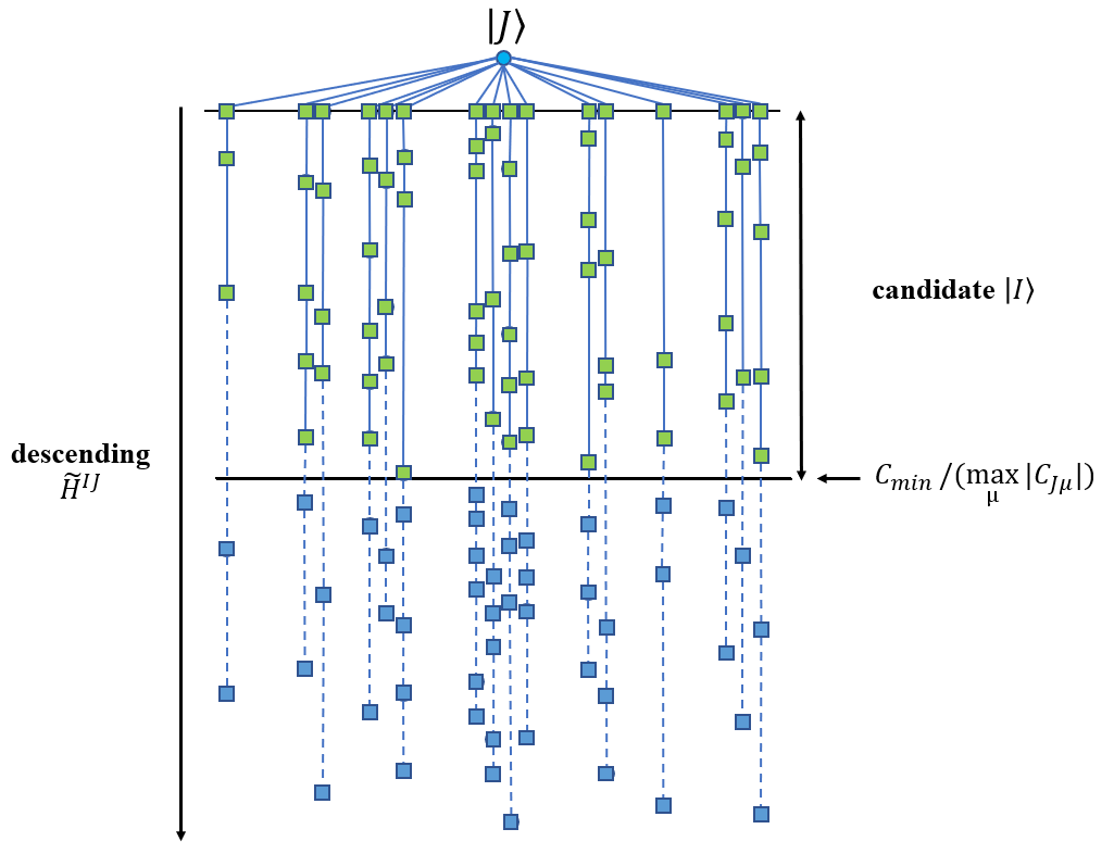
It should be clear that, for the same $C_{min}$, the revised ‘iCI criterion’ (28)/(29) will yield a smaller number of CSFs than the original one (26)/(27), for the latter may accumulate those CSFs of small coefficients until the condition is fulfilled (cf. the second sum in Eq. (26)), whereas the former just picks up the CSF with the largest coefficient. Note in passing that, to be compared directly with this ‘iCI criterion’, the ‘HBCI criterion’ (25) should be rewritten as

1. (a)

   If $|I\rangle$ is identical with or singly excited from $|J\rangle$, then

   $$f(|I\mu\rangle,|J\rangle,C_{min})=\max_{\nu}(|H^{IJ}_{\mu\nu}C_{J\nu}|)\geq C_{min};$$

   (30)

2. (b)

   If $|I\rangle$ is doubly excited from $|J\rangle$, then

   $$f(|I\mu\rangle,|J\rangle,C_{min})=\left(\max_{\nu}(|\tilde{H}^{IJ}C_{J\nu}|)\geq C_{min}\right)\text{ and }\left(\max_{\nu}(|H^{IJ}_{\mu\nu}C_{J\nu}|)\geq C_{min}\right),$$

   (31)

which amounts to skipping the final step in Eqs. (28)/(29).

References

- Liu (2020) Liu, W. Essentials of relativistic quantum chemistry. J. Chem. Phys. 2020, 152, 180901.
- Liu (2020) Liu, W. Relativistic quantum chemistry: today and tomorrow. Sci. Sin. Chim. 2020, DOI: 10.1360/SSC–2020–0120.
- Chaudhuri et al. (2005) Chaudhuri, R. K.; Freed, K. F.; Hose, G.; Piecuch, P.; Kowalski, K.; Włoch, M.; Chattopadhyay, S.; Mukherjee, D.; Rolik, Z.; Szabados, Á.; Tóth, G.; Surján, P. R. Comparison of low-order multireference many-body perturbation theories. J. Chem. Phys. 2005, 122, 134105.
- Hoffmann et al. (2009) Hoffmann, M. R.; Datta, D.; Das, S.; Mukherjee, D.; Szabados, Á.; Rolik, Z.; Surján, P. R. Comparative study of multireference perturbative theories for ground and excited states. J. Chem. Phys. 2009, 131, 204104.
- Lyakh et al. (2012) Lyakh, D. I.; Musiaz, M.; Lotrich, V. F.; Bartlett, R. J. Multireference nature of chemistry: The coupled-cluster view. Chem. Rev. 2012, 112, 182–243.
- Sherrill and Schaefer III (1999) Sherrill, C. D.; Schaefer III, H. F. The configuration interaction method: Advances in highly correlated approaches. Adv. Quantum Chem. 1999, 34, 143–269.
- Szalay et al. (2012) Szalay, P. G.; Muller, T.; Gidofalvi, G.; Lischka, H.; Shepard, R. Multiconfiguration self-consistent field and multireference configuration interaction methods and applications. Chem. Rev. 2012, 112, 108–181.
- Lischka et al. (2018) Lischka, H.; Nachtigallova, D.; Aquino, A. J.; Szalay, P. G.; Plasser, F.; Machado, F. B.; Barbatti, M. Multireference approaches for excited states of molecules. Chem. Rev. 2018, 118, 7293–7361.
- Liu and Hoffmann (2016) Liu, W.; Hoffmann, M. R. iCI: Iterative CI toward full CI. J. Chem. Theory Comput. 2016, 12, 1169–1178, (E) 2016, 12, 3000.
- White (1992) White, S. R. Density matrix formulation for quantum renormalization groups. Phys. Rev. Lett. 1992, 69, 2863.
- White (1993) White, S. R. Density-matrix algorithms for quantum renormalization groups. Phys. Rev. B 1993, 48, 10345–10356.
- White and Martin (1999) White, S. R.; Martin, R. L. Ab initio quantum chemistry using the density matrix renormalization group. J. Chem. Phys. 1999, 110, 4127–4130.
- Mitrushenkov et al. (2001) Mitrushenkov, A. O.; Fano, G.; Ortolani, F.; Linguerri, R.; Palmieri, P. Quantum chemistry using the density matrix renormalization group. J. Chem. Phys. 2001, 115, 6815–6821.
- Chan and Head-Gordon (2002) Chan, G. K.-L.; Head-Gordon, M. Highly correlated calculations with a polynomial cost algorithm: A study of the density matrix renormalization group. J. Chem. Phys. 2002, 116, 4462–4476.
- Chan and Sharma (2011) Chan, G. K.-L.; Sharma, S. The density matrix renormalization group in quantum chemistry. Annu. Rev. Phys. Chem. 2011, 62, 465–481.
- Sharma and Chan (2012) Sharma, S.; Chan, G. K.-L. Spin-adapted density matrix renormalization group algorithms for quantum chemistry. J. Chem. Phys. 2012, 136, 124121.
- Wouters and Van Neck (2014) Wouters, S.; Van Neck, D. The density matrix renormalization group for ab initio quantum chemistry. Eur. Phys. J. D 2014, 68, 272.
- Olivares-Amaya et al. (2015) Olivares-Amaya, R.; Hu, W.; Nakatani, N.; Sharma, S.; Yang, J.; Chan, G. K.-L. The ab-initio density matrix renormalization group in practice. J. Chem. Phys. 2015, 142, 034102.
- Li and Chan (2017) Li, Z.; Chan, G. K.-L. Spin-Projected Matrix Product States: Versatile Tool for Strongly Correlated Systems. J. Chem. Theory Comput. 2017, 13, 2681–2695.
- Baiardi and Reiher (2020) Baiardi, A.; Reiher, M. The density matrix renormalization group in chemistry and molecular physics: Recent developments and new challenges. J. Chem. Phys. 2020, 152, 040903.
- Booth et al. (2009) Booth, G. H.; Thom, A. J. W.; Alavi, A. Fermion Monte Carlo without fixed nodes: A game of life, death, and annihilation in Slater determinant space. J. Chem. Phys. 2009, 131, 054106.
- Cleland et al. (2010) Cleland, D.; Booth, G. H.; Alavi, A. Communications: Survival of the fittest: Accelerating convergence in full configuration-interaction quantum Monte Carlo. J. Chem. Phys. 2010, 132, 041103.
- Blunt et al. (2017) Blunt, N.; Booth, G. H.; Alavi, A. Density matrices in full configuration interaction quantum Monte Carlo: Excited states, transition dipole moments, and parallel distribution. J. Chem. Phys. 2017, 146, 244105.
- Petruzielo et al. (2012) Petruzielo, F. R.; Holmes, A. A.; Changlani, H. J.; Nightingale, M. P.; Umrigar, C. J. Semistochastic projector monte carlo method. Phys. Rev. Lett. 2012, 109, 230201.
- Holmes et al. (2016) Holmes, A. A.; Changlani, H. J.; Umrigar, C. J. Efficient heat-bath sampling in Fock space. J. Chem. Theory Comput. 2016, 12, 1561–1571.
- Ten-no (2013) Ten-no, S. Stochastic determination of effective Hamiltonian for the full configuration interaction solution of quasi-degenerate electronic states. J. Chem. Phys. 2013, 138, 164126.
- Ghanem et al. (2019) Ghanem, K.; Lozovoi, A. Y.; Alavi, A. Unbiasing the initiator approximation in full configuration interaction quantum Monte Carlo. J. Chem. Phys. 2019, 151, 224108.
- Blunt (2019) Blunt, N. S. A hybrid approach to extending selected configuration interaction and full configuration interaction quantum Monte Carlo. J. Chem. Phys. 2019, 151, 174103.
- Dobrautz et al. (2019) Dobrautz, W.; Smart, S. D.; Alavi, A. Efficient formulation of full configuration interaction quantum Monte Carlo in a spin eigenbasis via the graphical unitary group approach. J. Chem. Phys. 2019, 151, 094104.
- Neufeld and Thom (2020) Neufeld, V. A.; Thom, A. J. Accelerating Convergence in Fock Space Quantum Monte Carlo Methods. J. Chem. Theory Comput. 2020, 16, 1503–1510.
- Deustua et al. (2018) Deustua, J. E.; Magoulas, I.; Shen, J.; Piecuch, P. Communication: Approaching exact quantum chemistry by cluster analysis of full configuration interaction quantum Monte Carlo wave functions. J. Chem. Phys. 2018, 149, 151101.
- Lyakh and Bartlett (2010) Lyakh, D. I.; Bartlett, R. J. An adaptive coupled-cluster theory:@CC approach. J. Chem. Phys. 2010, 133, 244112.
- Xu et al. (2018) Xu, E.; Uejima, M.; Ten-no, S. L. Full Coupled-Cluster Reduction for Accurate Description of Strong Electron Correlation. Phys. Rev. Lett. 2018, 121, 113001.
- Xu et al. (2020) Xu, E.; Uejima, M.; Ten-No, S. L. Towards near-exact solutions of molecular electronic structure: Full coupled-cluster reduction with a second-order perturbative correction. J. Phys. Chem. Lett. 2020, 11, 9775–9780.
- Zhang and Evangelista (2016) Zhang, T.; Evangelista, F. A. A deterministic projector configuration interaction approach for the ground state of quantum many-body systems. J. Chem. Theory Comput. 2016, 12, 4326–4337.
- Eriksen et al. (2017) Eriksen, J. J.; Lipparini, F.; Gauss, J. Virtual orbital many-body expansions: A possible route towards the full configuration interaction limit. J. Phys. Chem. Lett. 2017, 8, 4633–4639.
- Eriksen and Gauss (2018) Eriksen, J. J.; Gauss, J. Many-Body Expanded Full Configuration Interaction. I. Weakly Correlated Regime. J. Chem. Theory Comput. 2018, 14, 5180–5191.
- Eriksen and Gauss (2019) Eriksen, J. J.; Gauss, J. Many-Body Expanded Full Configuration Interaction. II. Strongly Correlated Regime. J. Chem. Theory Comput. 2019, 15, 4873–4884.
- Eriksen and Gauss (2019) Eriksen, J. J.; Gauss, J. Generalized Many-Body Expanded Full Configuration Interaction Theory. J. Phys. Chem. Lett. 2019, 10, 7910–7915.
- Zimmerman (2017) Zimmerman, P. M. Incremental full configuration interaction. J. Chem. Phys. 2017, 146, 104102.
- Zimmerman (2017) Zimmerman, P. M. Strong correlation in incremental full configuration interaction. J. Chem. Phys. 2017, 146, 224104.
- Fales et al. (2018) Fales, B. S.; Seritan, S.; Settje, N. F.; Levine, B. G.; Koch, H.; Martínez, T. J. Large-Scale Electron Correlation Calculations: Rank-Reduced Full Configuration Interaction. J. Chem. Theory Comput. 2018, 14, 4139–4150.
- Greene et al. (2019) Greene, S. M.; Webber, R. J.; Weare, J.; Berkelbach, T. C. Beyond walkers in stochastic quantum chemistry: reducing error using fast randomized iteration. J. Chem. Theory Comput. 2019, 15, 4834–4850.
- Bytautas and Ruedenberg (2004) Bytautas, L.; Ruedenberg, K. Correlation energy extrapolation by intrinsic scaling. I. Method and application to the neon atom. J. Chem. Phys. 2004, 121, 10905–10918.
- Bytautas and Ruedenberg (2004) Bytautas, L.; Ruedenberg, K. Correlation energy extrapolation by intrinsic scaling. II. The water and the nitrogen molecule. J. Chem. Phys. 2004, 121, 10919–10934.
- Greer (1998) Greer, J. C. Monte Carlo configuration interaction. J. Comput. Phys. 1998, 146, 181–202.
- Coe and Paterson (2012) Coe, J. P.; Paterson, M. J. Development of Monte Carlo configuration interaction: Natural orbitals and second-order perturbation theory. J. Chem. Phys. 2012, 137, 204108.
- Ohtsuka and Hasegawa (2017) Ohtsuka, Y.; Hasegawa, J.-y. Selected configuration interaction method using sampled first-order corrections to wave functions. J. Chem. Phys. 2017, 147, 034102.
- Coe (2018) Coe, J. P. Machine Learning Configuration Interaction. J. Chem. Theory Comput. 2018, 14, 5739–5749.
- Holmes et al. (2016) Holmes, A. A.; Tubman, N. M.; Umrigar, C. J. Heat-bath configuration interaction: an efficient selected configuration interaction algorithm inspired by heat-bath sampling. J. Chem. Theory Comput. 2016, 12, 3674–3680.
- Garniron et al. (2017) Garniron, Y.; Scemama, A.; Loos, P.-F.; Caffarel, M. Hybrid stochastic-deterministic calculation of the second-order perturbative contribution of multireference perturbation theory. J. Chem. Phys. 2017, 147, 034101.
- Holmes et al. (2017) Holmes, A. A.; Umrigar, C. J.; Sharma, S. Excited states using semistochastic heat-bath configuration interaction. J. Chem. Phys. 2017, 147, 164111.
- Sharma et al. (2017) Sharma, S.; Holmes, A. A.; Jeanmairet, G.; Alavi, A.; Umrigar, C. J. Semistochastic Heat-Bath Configuration Interaction Method: Selected Configuration Interaction with Semistochastic Perturbation Theory. J. Chem. Theory Comput. 2017, 13, 1595–1604.
- Chien et al. (2018) Chien, A. D.; Holmes, A. A.; Otten, M.; Umrigar, C. J.; Sharma, S.; Zimmerman, P. M. Excited States of Methylene, Polyenes, and Ozone from Heat-Bath Configuration Interaction. J. Phys. Chem. A 2018, 122, 2714–2722.
- Yao et al. (2020) Yao, Y.; Giner, E.; Li, J.; Toulouse, J.; Umrigar, C. Almost exact energies for the Gaussian-2 set with the semistochastic heat-bath configuration interaction method. J. Chem. Phys. 2020, 153, 124117.
- Evangelista (2014) Evangelista, F. A. Adaptive multiconfigurational wave functions. J. Chem. Phys. 2014, 140, 124114.
- Schriber and Evangelista (2016) Schriber, J. B.; Evangelista, F. A. Communication: An adaptive configuration interaction approach for strongly correlated electrons with tunable accuracy. J. Chem. Phys. 2016, 144, 161106.
- Schriber and Evangelista (2017) Schriber, J. B.; Evangelista, F. A. Adaptive configuration interaction for computing challenging electronic excited states with tunable accuracy. J. Chem. Theory Comput. 2017, 13, 5354–5366.
- Schriber et al. (2018) Schriber, J. B.; Hannon, K. P.; Li, C.; Evangelista, F. A. A Combined Selected Configuration Interaction and Many-Body Treatment of Static and Dynamical Correlation in Oligoacenes. J. Chem. Theory Comput. 2018, 14, 6295–6305.
- Tubman et al. (2016) Tubman, N. M.; Lee, J.; Takeshita, T. Y.; Head-Gordon, M.; Whaley, K. B. A deterministic alternative to the full configuration interaction quantum Monte Carlo method. J. Chem. Phys. 2016, 145, 044112.
- Lehtola et al. (2017) Lehtola, S.; Tubman, N. M.; Whaley, K. B.; Head-Gordon, M. Cluster decomposition of full configuration interaction wave functions: A tool for chemical interpretation of systems with strong correlation. J. Chem. Phys. 2017, 147, 154105.
- Tubman et al. (2020) Tubman, N. M.; Freeman, C. D.; Levine, D. S.; Hait, D.; Head-Gordon, M.; Whaley, K. B. Modern approaches to exact diagonalization and selected configuration interaction with the adaptive sampling CI method. J. Chem. Theory Comput. 2020, 16, 2139–2159.
- Tubman et al. (2018) Tubman, N. M.; Levine, D. S.; Hait, D.; Head-Gordon, M.; Whaley, K. B. An efficient deterministic perturbation theory for selected configuration interaction methods. 2018, arXiv preprint arXiv:1808.02049.
- Liu and Hoffmann (2014) Liu, W.; Hoffmann, M. R. SDS: the ‘static-dynamic-static’ framework for strongly correlated electrons. Theor. Chem. Acc. 2014, 133, 1481.
- Lei et al. (2017) Lei, Y.; Liu, W.; Hoffmann, M. R. Further development of SDSPT2 for strongly correlated electrons. Mol. Phys. 2017, 115, 2696–2707.
- Zhang et al. (2020) Zhang, N.; Liu, W.; Hoffmann, M. R. Iterative Configuration Interaction with Selection. J. Chem. Theory Comput. 2020, 16, 2296–2316.
- Garniron et al. (2018) Garniron, Y.; Scemama, A.; Giner, E.; Caffarel, M.; Loos, P.-F. Selected configuration interaction dressed by perturbation. J. Chem. Phys. 2018, 149, 064103.
- Wang et al. (2019) Wang, Z.; Li, Y.; Lu, J. Coordinate descent full configuration interaction. J. Chem. Theory Comput. 2019, 15, 3558–3569.
- Giner et al. (2016) Giner, E.; Assaraf, R.; Toulouse, J. Quantum Monte Carlo with reoptimised perturbatively selected configuration-interaction wave functions. Mol. Phys. 2016, 114, 910–920.
- Scemama et al. (2018) Scemama, A.; Benali, A.; Jacquemin, D.; Caffarel, M.; Loos, P.-F. Excitation energies from diffusion Monte Carlo using selected configuration interaction nodes. J. Chem. Phys. 2018, 149, 034108.
- Bender and Davidson (1969) Bender, C. F.; Davidson, E. R. Studies in configuration interaction: The first-row diatomic hydrides. Phys. Rev. 1969, 183, 23.
- Whitten and Hackmeyer (1969) Whitten, J. L.; Hackmeyer, M. Configuration interaction studies of ground and excited states of polyatomic molecules. I. The CI formulation and studies of formaldehyde. J. Chem. Phys. 1969, 51, 5584–5596.
- Huron et al. (1973) Huron, B.; Malrieu, J. P.; Rancurel, P. Iterative perturbation calculations of ground and excited state energies from multiconfigurational zeroth-order wave functions. J. Chem. Phys. 1973, 58, 5745–5759.
- Evangelisti et al. (1983) Evangelisti, S.; Daudey, J. P.; Malrieu, J. P. Convergence of an improved CIPSI algorithm. Chem. Phys. 1983, 75, 91–102.
- Buenker and Peyerimhoff (1974) Buenker, R. J.; Peyerimhoff, S. D. Individualized configuration selection in CI calculations with subsequent energy extrapolation. Theor. Chem. Acta 1974, 35, 33–58.
- Eriksen et al. (2020) Eriksen, J. J.; Anderson, T. A.; Deustua, J. E.; Ghanem, K.; Hait, D.; Hoffmann, M. R.; Lee, S.; Levine, D. S.; Magoulas, I.; Shen, J.; Tubman, N. M.; Whaley, K. B.; Xu, E.; Yao, Y.; Zhang, N.; Alavi, A.; Chan, G. K.-L.; Head-Gordon, M.; Liu, W.; Piecuch, P.; Sharma, S.; Ten-no, S. L.; Umrigar, C. J.; Gauss, J. The ground state electronic energy of benzene. J. Phys. Chem. Lett. 2020, 11, 8922–8929.
- (77) Detail of timsort. https://en.wikipedia.org/wiki/Timsort.
- (78) https://github.com/timsort/cpp-TimSort.
- Buenker (1980) Buenker, R. J. In Molecular Physics and Quantum Chemistry: into the 80’s; Burton, P. G., Ed.; University of Wollongong Press: Wollongong, Australia, 1980; pp 1.5.1–1.5.37.
- Buenker (1986) Buenker, R. J. Combining perturbation theory techniques with variational CI calculations to study molecular excited states. Int. J. Quantum Chem. 1986, 29, 435–460.
- Krebs and Buenker (1995) Krebs, S.; Buenker, R. J. A new table-direct configuration interaction method for the evaluation of Hamiltonian matrix elements in a basis of linear combinations of spin-adapted functions. J. Chem. Phys. 1995, 103, 5613–5629.
- (82) Khait, Y. G.; Hoffmann, M. R. Low-Lying Potential Energy Surfaces; Chapter 8, pp 176–198.
- Huang et al. (2017) Huang, C.; Liu, W.; Xiao, Y.; Hoffmann, M. R. iVI: An iterative vector interaction method for large eigenvalue problems. J. Comput. Chem. 2017, 38, 2481–2499, (E) 2018, 39, 338.
- (84) Song, Y.; Guo, Y.; Lei, Y.; Liu, W. Benchmarking SDSPT2 and SDSCI for low-lying excited states of closed- and open-shell oragnic molecules. (unpublished).
- Huang and Liu (2019) Huang, C.; Liu, W. iVI-TD-DFT: An iterative vector interaction method for exterior/interior roots of TD-DFT. J. Comput. Chem. 2019, 40, 1023–1037, (E) 2018, 39, 338.
- Paldus (1974) Paldus, J. Group theoretical approach to the configuration interaction and perturbation theory calculations for atomic and molecular systems. J. Chem. Phys. 1974, 61, 5321–5330.
- Paldus and Boyle (1980) Paldus, J.; Boyle, M. J. Unitary group approach to the many-electron correlation problem via graphical methods of spin algebras. Phys. Script. 1980, 21, 295–311.
- Shavitt (1981) Shavitt, I. In The Unitary Group for the Evaluation of Electronic Energy Matrix Elements, 1st ed.; Hinze, J., Ed.; Lecture Notes in Chemistry 22; Springer-Verlag Berlin Heidelberg, 1981; pp 1–50.
- Shavitt (1977) Shavitt, I. Graph theoretical concepts for the unitary group approach to the many-electron correlation problem. Int. J. Quantum Chem., Symp. 1977, 12, 131–148.
- Duch and Karwowski (1985) Duch, W.; Karwowski, J. Symmetric group approach to configuration interaction methods. Comp. Phys. Rep. 1985, 2, 93–170.
- Shavitt (1978) Shavitt, I. Matrix element evaluation in the unitary group approach to the electron correlation problem. Int. J. Quantum Chem. 1978, 14, 5–32.
- Stampfuß and Wenzel (2005) Stampfuß, P.; Wenzel, W. Improved implementation and application of the individually selecting configuration interaction method. J. Chem. Phys. 2005, 122, 024110.
- Smith et al. (2017) Smith, J. E. T.; Mussard, B.; Holmes, A. A.; Sharma, S. Cheap and near exact CASSCF with large active spaces. J. Chem. Theory Comput. 2017, 13, 5468–5478.
- Li et al. (2020) Li, J.; Yao, Y.; Holmes, A. A.; Otten, M.; Sun, Q.; Sharma, S.; Umrigar, C. J. Accurate many-body electronic structure near the basis set limit: Application to the chromium dimer. Phys. Rev. Research 2020, 2, 012015(R).
- Schäfer et al. (1992) Schäfer, A.; Horn, H.; Ahlrichs, R. Fully optimized contracted Gaussian basis sets for atoms Li to Kr. J. Chem. Phys. 1992, 97, 2571–2577.
- Liu et al. (1997) Liu, W.; Hong, G.; Dai, D.; Li, L.; Dolg, M. The Beijing 4-component density functional theory program package (BDF) and its application to EuO, EuS, YbO and YbS. Theor. Chem. Acc. 1997, 96, 75–83.
- Liu et al. (2003) Liu, W.; Wang, F.; Li, L. J. Theor. Comput. Chem. 2003, 2, 257–272.
- Liu et al. (2004) Liu, W.; Wang, F.; Li, L. In Recent Advances in Relativistic Molecular Theory; Hirao, K., Ishikawa, Y., Eds.; World Scientific: Singapore, 2004; pp 257–282.
- Liu et al. (2004) Liu, W.; Wang, F.; Li, L. In Encyclopedia of Computational Chemistry; von Ragué Schleyer, P., Allinger, N. L., Clark, T., Gasteiger, J., Kollman, P. A., Schaefer III, H. F., Eds.; Wiley: Chichester, UK, 2004.
- Zhang et al. (2020) Zhang, Y.; Suo, B.; Wang, Z.; Zhang, N.; Li, Z.; Lei, Y.; Zou, W.; Gao, J.; Peng, D.; Pu, Z.; Xiao, Y.; Sun, Q.; Wang, F.; Ma, Y.; Wang, X.; Guo, Y.; Liu, W. BDF: A relativistic electronic structure program package. J. Chem. Phys. 2020, 152, 064113.
- Booth et al. (2014) Booth, G. H.; Smart, S. D.; Alavi, A. Linear-scaling and parallelisable algorithms for stochastic quantum chemistry. Mol. Phys. 2014, 112, 1855–1869.
- Li et al. (2018) Li, J.; Otten, M.; Holmes, A. A.; Sharma, S.; Umrigar, C. J. Fast semistochastic heat-bath configuration interaction. J. Chem. Phys. 2018, 149, 214110.
- Guo et al. (2018) Guo, S.; Li, Z.; Chan, G. K.-L. A Perturbative Density Matrix Renormalization Group Algorithm for Large Active Spaces. J. Chem. Theory Comput. 2018, 14, 4063–4071.
- Li et al. (2012) Li, Z.; Xiao, Y.; Liu, W. On the spin separation of algebraic two-component relativistic Hamiltonians. J. Chem. Phys. 2012, 137, 154114.
- Li et al. (2014) Li, Z.; Xiao, Y.; Liu, W. On the spin separation of algebraic two-component relativistic Hamiltonians: Molecular properties. J. Chem. Phys. 2014, 141, 054111.
- Balabanov and Peterson (2005) Balabanov, N. B.; Peterson, K. A. Systematically convergent basis sets for transition metals. I. All-electron correlation consistent basis sets for the 3d elements Sc–Zn. J. Chem. Phys. 2005, 123, 064107.
- (107) Li, Z. (priviate communication).