Data-driven Accelerogram Synthesis using Deep Generative Models
Abstract
Robust estimation of ground motions generated by scenario earthquakes is critical for many engineering applications. We leverage recent advances in Generative Adversarial Networks (GANs) to develop a new framework for synthesizing earthquake acceleration time histories. Our approach extends the Wasserstein GAN formulation to allow for the generation of ground-motions conditioned on a set of continuous physical variables. Our model is trained to approximate the intrinsic probability distribution of a massive set of strong-motion recordings from Japan. We show that the trained generator model can synthesize realistic 3-Component accelerograms conditioned on magnitude, distance, and . Our model captures the expected statistical features of the acceleration spectra and waveform envelopes. The output seismograms display clear P and S-wave arrivals with the appropriate energy content and relative onset timing. The synthesized Peak Ground Acceleration (PGA) estimates are also consistent with observations. We develop a set of metrics that allow us to assess the training process’s stability and tune model hyperparameters. We further show that the trained generator network can interpolate to conditions where no earthquake ground motion recordings exist. Our approach allows the on-demand synthesis of accelerograms for engineering purposes.
1 Introduction
Ground motion time histories are a critical input for many engineering design tasks (Heaton et al. 1986). Under specific circumstances, modern construction codes make it compulsory to perform time-history analysis of a building’s structural response (Bommer & Acevedo 2004). Synthesizing realistic acceleration time-series remains a formidable challenge (Graves & Pitarka 2010; Douglas & Aochi 2008); practicing engineers still use past earthquakes recordings to represent the expected ground motions that would be generated by scenario events (Hancock et al. 2008; Hancock et al. 2006). The assumption that future shaking will be similar to that observed in the past is well-grounded and typically valid. Nevertheless, careful scaling and selection of records, as well as ease of access to databanks, are required to apply this technique successfully. Given the recent explosion in seismological data collection and the many exciting developments in modern machine learning, the idea that an artificial intelligence system could provide on-demand, accurate and realistic ground motion time histories for engineering purposes is not farfetched.
While advances in our understanding of the complex rupture and wave propagation processes that cause the ground motions observed at the surface make the prospect of numerically simulating realistic strong motions increasingly likely, fundamental limitations remain. The exponential growth in computing power and the development of efficient and accurate numerical methods (Graves 1996; Komatitsch & Vilotte 1998), make it possible to model wave propagation through 3-D heterogeneous media. If an accurate velocity model is available, elastodynamic Green’s functions for frequencies as high as 1 Hz can be calculated with relative ease. Once a reasonable approximation of the Green’s function is obtained, the rupture process has to be modeled. A kinematic source description is often used (Herrero & Bernard 1994); the hypothetical fault is divided into patches or sub-faults, and the relevant physical parameters (e.g., slip, rupture velocity, rise time) must be either known or assumed for each sub-fault (Graves & Pitarka 2010). A fully dynamic rupture simulation could capture the fundamental physical processes that drive faulting, and thus it would require a smaller number of well-constrained parameters; it is a promising alternative, actively researched, but still unavailable for any practical purposes (Mena et al. 2012). Current simulation methods account for large structures (Ma et al. 2007), such as sedimentary basins, but do not capture small scale heterogeneities responsible for local site effects (Graves & Pitarka 2010) and seismogram coda, which control the shape of the Fourier Amplitude Spectrum of accelerograms. Our lack of detailed knowledge of the earth’s structure also poses a significant challenge; 3-D velocity models are notoriously difficult to constrain and only available for a handful of regions.
When the computational cost of deterministic simulations was prohibitive and observational datasets were small, sparse, and difficult to access (Douglas & Aochi 2008), stochastic modeling methods were the only viable alternative. Initially developed for engineering purposes (Kaul 1978; Gasparini & Vanmarcke 1976; Naeim & Lew 1995). In their most basic form, white Gaussian noise is windowed and filtered, modified in the frequency domain, and then transformed back to the time domain, where it is multiplied by an envelope function (Naeim & Lew 1995). The process is iterative, and the goal used to be that of matching a design response spectrum (Naeim & Lew 1995). Pioneering work by Boore 1983; Boore 2003 extended and formalized this approach for point sources by considering simple physical models (Boore 1983). The source spectrum is assumed to have a random phase (Hanks & McGuire 1981), but instead of using ad hoc manipulations, spectral amplitudes are modified to approximate the acceleration spectrum proposed by Brune 1970, simplified theoretical representations of Path and Site effects are also needed. When transforming back to the time domain, an appropriate envelope function, reflecting source duration, must be carefully chosen (Boore 2003). This approach can readily be extended to finite faults and does provide reasonable high-frequency approximations for single-phase arrivals (Herrero & Bernard 1994). Unfortunately, it can not generate coherent 3-Component waveforms with multiple arrivals and coda typical of real earthquakes (Douglas & Aochi 2008); it completely ignores phase effects, and it does not accurately represent long period motions (Graves & Pitarka 2010). Given these limitations, substantially more involved hybrid methods exist, in which low-frequency waveforms are simulated deterministically, while high-frequency effects are modeled stochastically (Graves & Pitarka 2010).
We present a novel data-driven framework for synthesizing ground motion time histories. We train a generator model to learn an optimal probabilistic representation of observed acceleration time-series directly from a strong-motion dataset. In section 2, we review some of the concepts necessary to understand or approach. Section 3 presents the details of the technique and model architecture. Section 4 describes the training dataset and our choice of input variables. The result’s section shows that our approach generalizes well, even when no data is available for specific event-station distance and earthquake magnitude ranges, and it also introduces a metric for assessing the training process’s convergence; we focus on displaying examples and assessing the quality of our model for distances and magnitudes relevant to engineering applications. Finally, we discuss the advantages and potential limitations of our framework.
2 Background on GANs
Generative models are a class of statistical models that attempt to capture the underlying probability distribution of a dataset. In particular, they are trained to produce data that looks as if it was sampled from the original training set (Bengio et al. 2013a; Alain & Bengio 2014). Data generation is harder than any classification or prediction task (Bengio et al. 2013). A useful generative model has to adequately capture most of the correlations in data space. When learning to produce images of human faces, for example, a model must learn a data boundary: a human face only has two eyes, but it also has to position them below the forehead and place a nose in between. If the task is to synthesize seismograms, the S wave must come after the P wave, but more importantly, the statistical distribution of the data in frequency space should also be captured.
Generative Adversarial Networks (GANs) are state-of-the-art generative models (Goodfellow et al. 2014). Advances in architecture and training techniques have enabled GANs to synthesize high-resolution realistic-looking images of human faces (Karras et al. 2018), audio (Donahue et al. 2018) and even video sequences (Saito & Saito 2018). GANs are built using two networks that are trained simultaneously (Goodfellow et al. 2014): a discriminator network and a generator network . The discriminator is a binary classification model trained to determine whether its input came from the real data distribution or it was produced by . The generator maps samples from a Gaussian distribution into samples coming from a new implicitly defined distribution . The goal of the process is to make as close to as possible.
During training, the discriminator model is continuously refined; at each iteration, is shown samples generated by , which are labeled as , or ”fake” and data sampled from , labeled with a , or coming from the ”real” distribution. The generator, on the other hand, is constantly optimized with respect to , such that the samples it produces are classified as ”real” by the discriminator 1. Note that when the generator optimization step takes place, the weights of are kept fixed.
Despite the many successful implementations, issues such as instability and mode collapse make conventional GANs notoriously difficult to train (Salimans et al. 2016; Arjovsky & Bottou 2017). A given application might require substantial architectural refinement and hyperparameter tuning (Radford et al. 2015). Li et al. 2018 showed that, in principle, a GAN could be trained to generate synthetic seismograms. Unfortunately, their model was only able to capture the first 4 seconds of the P wave arrival. Wang et al. 2019 also showed that waveforms synthesized using a GAN are useful for data augmentation and that an enhanced training set can improve earthquake detectability. However, finding a generative model able to synthesize realistic earthquake ground motion time-series remains an open problem.

3 Methods
3.1 Wasserstein GANs
Most of the work on GANs was focused on finding architectures to bring stability into the training process until the work of Arjovsky et al. 2017 provided the necessary theoretical tools to understand adversarial training. Conventional GANs, as introduced by Goodfellow et al. 2014, attempt to minimize the Jensen-Shannon (JS) divergence between the data distribution and the distribution , implicitely defined by the generator model. Informally, the training instability arises from the fact that when and do not overlap, the JS divergence between them is not differentiable everywhere (Arjovsky & Bottou 2017). Furthermore, the discriminator can not be trained to optimality, as this would lead to increasingly small gradients Arjovsky et al. 2017.
Wasserstein Generative Adversarial Networks (WGANs) overcome many of the limitations mentioned earlier by using the Earth Mover’s (EM) distance as a measure of similarity between and (Arjovsky et al. 2017). Intuitively, the EM or Wasserstein-1 distance is the minimum cost of transporting the probability mass necessary to transform into the target distribution , where the cost is defined as mass times distance (Villani 2009). In the Wasserstein formulation the discriminator is trained to solve the fallowing optimization problem:
| (1) |
Where and implies that is sampled from a Gaussian distribution . This is equivalent to finding using the Kantorovich-Rubinstein duality (Villani 2009). The discriminator is no longer a binary classifier, it now acts as a critic, it outputs a real score that approximates the EM distance between and . The optimization problem in (1) has an important constraint, must be a 1-Lipschitz function, that is (Arjovsky et al. 2017):
| (2) |
For any input pair , which means that the gradient of the discriminator with respect to its inputs is bounded, its -norm can never exceed . Weight clipping is the most straight forward way to impose (2); unfortunately, it often leads to a coarse approximation of and to vanishing or exploding gradients when the clipping threshold is not carefully chosen.
We follow Gulrajani et al. 2017 and enforce the 1-Lipschitz constraint by adding a regularization term to the discriminator objective function:
| (3) |
Where is a constant, and is uniformly sampled along straight lines connecting points in and . Imposing the 1-Lipschitz constraint via sampling does not guarantee that it will be satisfied everywhere; however, it gives good results (Gulrajani et al. 2017), as it encourages the discriminator gradient norm to move towards in regions relevant to the problem, where gradients provide critical information for subsequent model updates. The generator is adversarially trained by minimizing the objective function:
| (4) |
As in the original GAN formulation, the generator weights are optimized with respect to the discriminator, and both models are trained simultaneously. The 1-Lipschitz constraint on means that it can and should be trained to optimality, so it is useful to perform a few optimization steps, , on the discriminator before the generator model is updated.
3.2 Conditional WGAN
We seek a model that can synthesize 3-Component accelerograms conditioned on a set of continuous input variables . Inspired by the success of Conditional Generative Adversarial Networks (cGAN) in many image generation tasks (Mirza & Osindero 2014), such as image to image translation (Isola et al. 2017), image super-resolution (Ledig et al. 2017) and text to image synthesis (Reed et al. 2016); we present an extension of the Wasserstein GAN formulation for the task of data generation using continuous conditional variables.
We construct a generator model to map normally distributed random noise and a set of continuous conditional variables into an accelerogram , (figure 2). The mapping implicitly defines a conditional probability distribution . The discriminator model also learns a mapping, , that approximates how close the distribution defined by is to the real conditional data distribution. Once more, the discriminator can be understood as a critic, trained to assess if the pair was sampled from the real distribution.
We empirically found that it was essential to use a separate embedding network for each of the conditional variables (figure 2). We designed each embedding as a four-layer fully connected neural network (FCNN) to map a continuous variable input to a higher dimensional representation. Both and had different embedding networks, whose weights were optimized during training. It is not clear why this is so critical, but probably, it is because learning is more effective when sparse high dimension data representations are used (Bengio et al. 2013a).
It was also important to train the discriminator to optimality, which was achieved by using a relatively large number of critic iterations, . We found that was necessary to bring stability to the training process. A value of is typically used for unconditional image generation (Arjovsky et al. 2017; Gulrajani et al. 2017), approximating the EM distance between conditional distributions might be a harder problem.

3.3 Model Architecture
The overall architecture follows the guidelines presented in (Radford et al. 2015), which have become standard practice when assembling deep convolutional GANs for image generation. The discriminator is implemented as a series of strided convolutions that progressively reduce the dimensionality of the input data, while increasing its depth, as the features relevant for classification are extracted. The generator starts from a gaussian noise vector that is progressively upsampled until an output with the same shape as the discriminator’s input is produced. In the formulation of Radford et al. 2015 upsampling is performed by a series of transpose convolutional layers, but we found this approach to be ineffective for synthesizing seismograms. Instead, we used a nearest-neighbor resize (NNR), followed by three successive convolutions (Odena et al. 2016). The NNR layer doubles the size of its input along the time dimension; the convolutional layers apply their filters while preserving their input’s dimension along the time axis.
In our architecture, the generator model is given a three-channel random normal vector of length 100 as input, the higher dimensional representation of each conditional variable is concatenated and added as an additional channel. We feed the result into two fully connected layers with 128 units each and then into two upsampling layers implemented as described earlier, where each convolution has a filter of size 5 and a stride of 1. All layers are followed by batch normalization (Ioffe & Szegedy 2015) and a ReLU activation function, except for the last one, where no normalization is applied, and is used as activation. outputs 20 second long, 3-component waveforms, sampled at .
The discriminator model takes a 3-component waveform, either real or synthesized by , and the set of continuous conditional variables as inputs. After each variable is passed through its corresponding embedding network, its high dimensional representation is added as an extra channel to the waveform. Four convolutional layers are followed by four fully connected layers. We apply Leaky ReLU activation functions and batch normalization, except for the input layer, which omits the normalization, and the output layer, which omits both. With no activation, the output yields raw non-normalized values. In this manner, acts as a critic that scores its input, as opposed to a typical discriminator which assigns probabilistic binary labels.
4 Data and Training
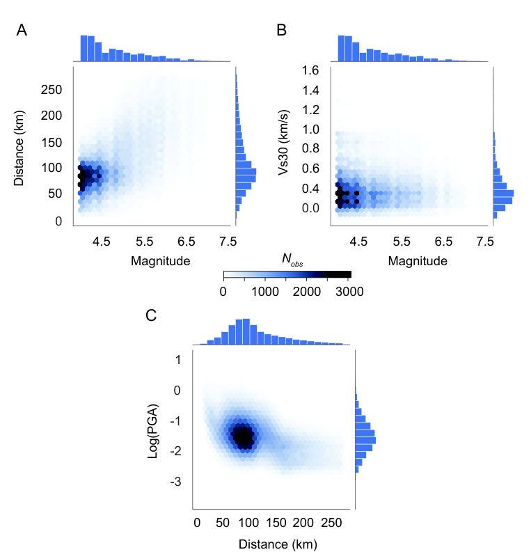
We assemble a set of strong-motion recordings from Japanese seismograph networks K-NET and KiK-Net, corresponding to earthquakes. We only use ground surface stations. We focus on signals useful for ground motion prediction and engineering applications (Douglas & Aochi 2008; Power et al. 2008) by selecting events with magnitudes between 4.0 and 7.5 at event-station distances between and .
We also collect available values of at each station. is defined as the shear wave speed averaged to a depth of 30m directly below the ground. It is the best-known proxy for the response of a site to an earthquake (Borcherdt 2012), and it is used in building codes worldwide to separate sites into different categories for design purposes.
Because of their relevance to ground motion prediction, and their high correlation with essential features of the ground motions generated at the surface, we select the following physical parameters as the conditional variables for our model (figure (4)):
- •
Event-Station Distance
- •
Earthquake Magnitude
- •
Vs30 at the recording station
Here we have focused on a minimal set of physical parameters whose impact on the observed seismograms can easily be quantified. These three variables are often the dominant terms in ground motion prediction equations (Douglas & Aochi 2008), which makes our approach a useful supplement, or alternative, to current prediction methodologies.
Before training, we further curate our dataset. The original ground motion recordings are sampled at ; we downsample them to and select 20-second windows that start 2.5 seconds before the P wave onset. The maximum Peak Ground Acceleration (PGA) in our dataset is . We also remove stations with less than 20 recorded accelerograms, as this could be indicative of potential instrumental issues.
We normalize each input channel to take values between (Radford et al. 2015). The log of the scaling factors is concatenated to the input accelerogram. Thus, we train our model to synthesize 3-component, 400 sample seismograms, along with their associated normalization factors. We use the Adam stochastic optimization algorithm and train the discriminator iterations for each generator optimization step. We let the process run for at least epochs and select the best model by using the criteria discussed in section 5.4 as well as visual inspection of averaged statistical aspects of the generated waveforms.
5 Results
5.1 Model Validation in Time and Frequency Domains
Our generator model is stochastic; our goal is not to provide a one-to-one correspondence between a set of variables and seismograms, or ground motion intensity measures, as in a typical regression problem. Instead, by approximating the intrinsic probability distribution of a regional ground motion dataset, we have built a model that allows us to sample 3-Component acceleration time-series vectors, , conditioned on a set of physically meaningful variables. As such, we can only assess the quality of our model in a statistical sense. Because we seek to synthesize realistically looking seismograms adequate for engineering applications, our generator model must perform well in both frequency and time domains. We evaluate our model in the frequency domain (FD) by comparing the average Fourier amplitudes of real and synthetic seismograms. The average spectra of a set of accelerograms in log-space is given by:
| (5) |
Where is the norm of the 3-Component vector of Fourier Amplitudes for accelerogram at frequency . We use a multitaper estimation technique to compute the spectrum of each accelerogram component (Prieto et al. 2009).
In the time domain (TD), we use average acceleration envelopes as our evaluation metric. The envelope of a seismogram is defined as . As before, we compute averages in log-space:
| (6) |
To compare our model predictions with statistical quantities computed on real accelerograms, we divide our dataset into discrete magnitude-distance-vs30 bins. We synthesize waveforms using the bin mid-points as inputs and, whenever possible, randomly select the same number of real accelerograms in the given bin for comparison. The generator was trained using continuous conditional variables as inputs; thus, an ideal testing design would require extremely narrow bins. (Figure 5). In practice, data availability limits the size of the bins. We used bin widths of in event-station distance and magnitude units. For , we relied on available data to select bin widths. Meaningful statistical comparisons are possible when a sufficiently large number of observations are available in each bin, at least 20. However, given the nature of earthquakes statistics, and the current design of strong-motion sensor networks, it is challenging to gather observations of large earthquakes , especially at short distances . Those cases are the most relevant for engineering applications; therefore, we were forced to compute TD and FD statistics using only a handful of real accelerograms in some situations. See Figure 5 for detailed comparisons in several representative frequency-magnitude-vs30 bins.

5.2 Peak Ground Acceleration
As discussed in section 4, the generator produces normalized 3-Component waveforms and their corresponding normalization factors. We take the Peak Ground Acceleration (PGA) as the maximum of the three normalization constants.
In Figure 6, we display as a function of distance for several representative magnitudes and fixed values of . We plot two panels, one for a soft site and other for hard bedrock . As a byproduct of our seismogram generation strategy, we have built a model that has many of the essential ingredients of Ground Motion Prediction Equations (GMPEs). Figure 7 displays physically reasonable, relatively smooth curves that capture the most relevant trends present in our dataset. Careful inspection of figure 7 reveals that our model could be used to calculate PGA in regions of the parameter space where no data is available. In the next section, we examine whether this is captured by the synthetic accelerograms, and the ability of the model to interpolate waveforms to conditions not previously observed.
5.3 Interpolation Experiment
We design a series of experiments to determine whether the generator model can be used to interpolate acceleration time histories to conditions where no earthquake ground motion recordings exist. We select a distance-magnitude-vs30 bin from the original dataset for each experiment, containing at least 30 observations and having a distance width of no more than . Figure’s 8 experiments focus on bins with large magnitude earthquakes, Supp. Figure 2 concentrates on bins with event-station distances less than . We remove all accelerograms belonging to the selected bin and retrain our model. The removed data is held out for subsequent testing. Once the generator model is trained, we use the bin mid-points to generate synthetic seismograms. We then compute average Fourier amplitude spectra, and average acceleration envelops for the synthetic and holdout sets. Finally, we calculate standard deviations in log-space and overlay the corresponding results in the same plot (Figure 8), which allows us to visually assess the generator’s model quality.
We perform an initial series of interpolation experiments using only two conditional variables: distance and magnitude (Supp. Figure 1). These two variables control most of the first-order features observed in accelerograms, e.g., the time difference between the first onset (P-wave) and the second one (S-wave) directly correlates with distance. Also, larger magnitude events have amplitude spectra with relatively more energy concentrated at lower frequencies, making visual validation of the results straight forward.
Distance and Magnitude are the essential ingredients of any ground motion prediction model. Hence, as a methodological strategy, we started by building a robust model using only these two variables and extended it by introducing an additional variable: Vs30, a proxy for site response. In Figure 8 and Supp. Figure 2, we show the results of our interpolation experiments run using our full model with its three conditional variables: distance, magnitude, and Vs30.

5.4 Training Stability and Hyperparameter tuning
A critical advantage of WGANs is that they provide a useful metric that correlates well with the quality of the generator output, the Wasserstein distance as approximated by the discriminator loss (Arjovsky & Bottou 2017):
| (7) |
Note that these are simply the first two terms in equation 3, but with the sign flipped, because is defined as a maximum, and during the optimization process we search for a minimum.
We perform a series of experiments to assess the sensitivity of the training process to different hyperparameter choices. In each experiment, we split our initial data into two randomly selected non-overlapping sets: 80% for training and 20 % for validation. We adversarially train our models about 160 epochs and compute on the training set after each generator iteration. The validation loss is computed after a full epoch. The training loss is a continuous snapshot of the optimization process, so it looks noisier; the validation loss, on the other hand, is a smooth average that allows us to assess the stability and the generalizability of our model.
In Figure 9, we show the results of four experiments where we vary the learning rate. Following (Gulrajani et al. 2017) we used an Adam optimizer (Kingma & Ba 2014) with and . We choose a learning rate of , much lower than the default because it gives stable results, and, among all experiments performed, it results in the smallest value. Equation 7 provides a useful metric to diagnose potential issues.
We also explore the effect of sample size (Figure 10), by randomly selecting subsets of observations from our original dataset. For , we observed no signs of convergence; instead, the validation and training losses tend to plateau at relatively high values of ; this behavior correlates with poor quality of the generated accelerograms, as shown in the first row of Figure 10. At output quality starts to improve, but even when using samples the trained model is not able to capture important details of the accelerogram’s envelop distribution. We conclude that at least samples are needed for our model to converge to realistically looking waveforms. These sample size experiments are specific to our dataset, but can serve as a guideline when applying our method to other regions.


6 Discussion and Conclusion
Generating realistic ground motion time histories for hypothetical earthquakes remains challenging. Deterministic simulation methods are promising but not yet practical. We have taken advantage of the increasing availability of strong-motion sensor data and recent advances in machine learning to propose a completely alternative approach. We developed an adversarial training scheme that allowed a generator deep neural network to learn the conditional probability distribution of a massive ground motion data set from Japan. Our results suggest that approximates well the many complex processes that give rise to the observed earthquake ground motions, the acceleration time series it synthesizes have all the essential ingredients of real accelerograms in both time and frequency domains (Figure 5 and Figure 3).
An advantage of our technique is that it directly captures site effects. Simulation-based methods typically model ground motions for reference bedrock sites; the resulting acceleration spectrum has to be modified in an ad-hoc fashion by multiplying it with empirically derived site-specific amplification factors. Our model synthesizes acceleration times series with Fourier amplitude spectral shapes that closely follow the ones of real accelerograms for different values (Figure 5 ). Interestingly, there is consistently more energy at lower frequencies (0.1-2 Hz) for smaller values of (). Our results confirm that vs30 is an excellent proxy for site response. It exerts an important control on Fourier amplitude spectral shapes; this is apparent from the data and the synthesized accelerograms (Figure 5 ).
A second distinguishing feature of our methodology is that it is stochastic by design. It does not produce a single waveform consistent with a set of input parameters; it provides a full range of possible ground motions that accurately reflect the data’s variability. There are two critical reasons for this: (1) learns to approximate a conditional probability distribution, and (2) our framework never attempts to fit the data in the time or the frequency domains. The adversarial training scheme allows the discriminator model to provide a dynamic measure of similarity that continuously improves. Thus, the synthesized acceleration time histories reflect the variability of potential ground motions in the region where the data was collected. Such a synthetic set of ground motions may allow engineering to perform dynamical analysis of structures in a Bayesian sense and to determine robust confidence intervals for their estimates.
As with any machine learning approach, the computational cost is paid upfront during training. Our model takes about 8 hours to train on an Nvidia Tesla V100 GPU, but once the process is complete, it can synthesize hundreds of accelerograms in seconds, even when running on modest laptop hardware. We provide a pre-trained generator model and open-source code so that any user can quickly synthesize ground motions of interest. Deterministic simulation of a single scenario earthquake has a computational cost orders of magnitude larger. It requires specialized High-Performance Computing (HPC) hardware not available to most users, and it is limited by the lack of detailed knowledge of the earth’s structure and rupture characteristics.
Our approach lays a foundation for data-driven synthesis of accelerograms, and we envision additional work in the future expanding on this framework. We have chosen a simple, functional model architecture for this study: 400 output units per channel, limiting us to 20-second long waveforms sampled at and three conditional input variables. We have proven that it works well for a wide range of scenario earthquakes in Japan. We have also provided all the necessary ingredients and guidance to adapt it to any other region’s data set. The conditional variables were chosen to reflect the key controlling factors of earthquake ground motions: Distance from the hypocenter, event size, and site response. Since our framework is stochastic, it may not be necessary or even desirable to include additional variables. The generator model already provides a full set of accelerograms representing many faulting styles, source characteristics, and relevant hypocentral depths. Furthermore, if needed, our framework can be combined with a suitable set of Ground Motion Prediction Equations (GMPEs); the model does provide reliable PGA estimates (Figure 6 and Figure 7), but it would be straight forward to use the normalized output waveforms along with PGA or PGV estimates obtained using regional GMPEs.
While our model has been shown to successfully interpolate waveforms given conditioning variables not seen before, its main limitation is that it cannot extrapolate outside of this range. Users of the trained model should be aware of this and plan subsequent usage of the model accordingly. For our dataset, the main concerns here are the high and low ends of the magnitude spectrum. As additional data become available in the future, it may be possible to expand this range. An additional minor challenge of our method currently is that in a handful of cases, our model struggles to approximate the first 2.5 seconds of noise before the p-wave onset. Inspection of envelope statistics of real accelerograms (Figure 5) reveals that pre-signal noise variability is often large, spanning many orders of magnitude. Therefore, the noise may come from different distributions, varying across stations, with a complex signature that is challenging to capture.
Longer accelerograms, with a potentially more accurate noise signature, can be synthesized by increasing the number of layers and the number of output units. Larger models tend to perform better but would take significantly longer to train. Since we had to iterate over a large number of network architectures and hyperparameter choices in a reasonable time, we kept our model as small as possible; nevertheless, given sufficient computing power, the same architecture can be readily scaled up.
The waveforms the generator model can synthesize are already appropriate for many engineering applications. We are confident that the framework we have developed is robust and well-suited for many ground-motion prediction tasks. Further work is still needed, but the goal of synthesizing on-demand, accurate acceleration time-histories for any scenario earthquake might be within reach.

References
- Brune (1970) James. Brune “Tectonic stress and the spectra of seismic shear waves from earthquakes” _eprint: https://agupubs.onlinelibrary.wiley.com/doi/pdf/10.1029/JB075i026p04997 In Journal of Geophysical Research (1896-1977) 75.26, 1970, pp. 4997–5009 DOI: 10.1029/JB075i026p04997
- Gasparini & Vanmarcke (1976) Dario Gasparini and Erik Vanmarcke “Simulated earthquake motions compatible with prescribed response spectra” OCLC: 1176024695 Cambridge, MA: Massachusetts Institute of Technology, Dept. of Civil Engineering, Constructed Facilities Division, 1976
- Kaul (1978) Maharaj. Kaul “Spectrum-Consistent Time-History Generation” Publisher: ASCE In Journal of the Engineering Mechanics Division 104.4, 1978, pp. 781–788 URL: https://cedb.asce.org/CEDBsearch/record.jsp?dockey=0008198
- Hanks & McGuire (1981) Thomas. Hanks and Robin. McGuire “The character of high-frequency strong ground motion” Publisher: GeoScienceWorld In Bulletin of the Seismological Society of America 71.6, 1981, pp. 2071–2095 URL: https://pubs.geoscienceworld.org/ssa/bssa/article/71/6/2071/102118/The-character-of-high-frequency-strong-ground
- Boore (1983) David. Boore “Stochastic simulation of high-frequency ground motions based on seismological models of the radiated spectra” Publisher: GeoScienceWorld In Bulletin of the Seismological Society of America 73.6, 1983, pp. 1865–1894 URL: https://pubs.geoscienceworld.org/ssa/bssa/article/73/6A/1865/118579/Stochastic-simulation-of-high-frequency-ground
- Heaton et al. (1986) Thomas. Heaton, Fumiko Tajima and Ann Mori “Estimating ground motions using recorded accelerograms” In Surveys in Geophysics 8.1, 1986, pp. 25–83 DOI: 10.1007/BF01904051
- Herrero & Bernard (1994) A. Herrero and P. Bernard “A kinematic self-similar rupture process for earthquakes” Publisher: GeoScienceWorld In Bulletin of the Seismological Society of America 84.4, 1994, pp. 1216–1228 URL: https://pubs.geoscienceworld.org/ssa/bssa/article/84/4/1216/119869/A-kinematic-self-similar-rupture-process-for
- Naeim & Lew (1995) Farzad Naeim and Marshall Lew “On the Use of Design Spectrum Compatible Time Histories” Publisher: SAGE Publications Ltd STM In Earthquake Spectra 11.1, 1995, pp. 111–127 DOI: 10.1193/1.1585805
- Graves (1996) Robert. Graves “Simulating seismic wave propagation in 3D elastic media using staggered-grid finite differences” Publisher: GeoScienceWorld In Bulletin of the Seismological Society of America 86.4, 1996, pp. 1091–1106 URL: https://pubs.geoscienceworld.org/ssa/bssa/article/86/4/1091/120141/Simulating-seismic-wave-propagation-in-3D-elastic
- Komatitsch & Vilotte (1998) Dimitri Komatitsch and Jean-Pierre Vilotte “The spectral element method: An efficient tool to simulate the seismic response of 2D and 3D geological structures” Publisher: GeoScienceWorld In Bulletin of the Seismological Society of America 88.2, 1998, pp. 368–392 URL: https://pubs.geoscienceworld.org/ssa/bssa/article/88/2/368/120304/The-spectral-element-method-An-efficient-tool-to
- Boore (2003) D.. Boore “Simulation of Ground Motion Using the Stochastic Method” In pure and applied geophysics 160.3, 2003, pp. 635–676 DOI: 10.1007/PL00012553
- Bommer & Acevedo (2004) Julian. Bommer and Ana Acevedo “The use of real earthquake accelerograms as input to dynamic analysis” Publisher: Imperial College Press In Journal of Earthquake Engineering 08, 2004, pp. 43–91 DOI: 10.1142/S1363246904001596
- Hancock et al. (2006) Jonathan Hancock et al. “An Improved Method of Matching Response Spectra of Recorded Earthquake Ground Motion Using Wavelets” In Journal of Earthquake Engineering 10, 2006, pp. 67–89 DOI: 10.1080/13632460609350629
- Ma et al. (2007) Shuo Ma, Ralph. Archuleta and Morgan. Page “Effects of Large-Scale Surface Topography on Ground Motions, as Demonstrated by a Study of the San Gabriel Mountains, Los Angeles, CaliforniaEffects of Large-Scale Surface Topography on Ground Motions” Publisher: GeoScienceWorld In Bulletin of the Seismological Society of America 97.6, 2007, pp. 2066–2079 DOI: 10.1785/0120070040
- Douglas & Aochi (2008) John Douglas and Hideo Aochi “A Survey of Techniques for Predicting Earthquake Ground Motions for Engineering Purposes” In Surveys in Geophysics 29.3, 2008, pp. 187 DOI: 10.1007/s10712-008-9046-y
- Hancock et al. (2008) Jonathan Hancock, Julian. Bommer and Peter. Stafford “Numbers of scaled and matched accelerograms required for inelastic dynamic analyses” In Earthquake Engineering & Structural Dynamics 37.14, 2008, pp. 1585–1607 DOI: 10.1002/eqe.827
- Power et al. (2008) Maurice Power et al. “An Overview of the NGA Project” Publisher: SAGE Publications Ltd STM In Earthquake Spectra 24.1, 2008, pp. 3–21 DOI: 10.1193/1.2894833
- Prieto et al. (2009) G.. Prieto, R.. Parker and F.. VernonIII “A Fortran 90 library for multitaper spectrum analysis” In Computers & Geosciences 35.8, 2009, pp. 1701–1710 DOI: 10.1016/j.cageo.2008.06.007
- Villani (2009) Cédric Villani “Optimal Transport: Old and New”, Grundlehren der mathematischen Wissenschaften Berlin Heidelberg: Springer-Verlag, 2009 DOI: 10.1007/978-3-540-71050-9
- Graves & Pitarka (2010) Robert. Graves and Arben Pitarka “Broadband Ground-Motion Simulation Using a Hybrid ApproachBroadband Ground-Motion Simulation Using a Hybrid Approach” Publisher: GeoScienceWorld In Bulletin of the Seismological Society of America 100.5, 2010, pp. 2095–2123 DOI: 10.1785/0120100057
- Borcherdt (2012) Roger. Borcherdt “VS30 – A site-characterization parameter for use in building Codes, simplified earthquake resistant design, GMPEs, and ShakeMaps”, 2012 URL: https://pubs.er.usgs.gov/publication/70041709
- Mena et al. (2012) B. Mena, L.. Dalguer and P.. Mai “Pseudodynamic Source Characterization for Strike‐Slip Faulting Including Stress Heterogeneity and Super‐Shear RupturesPseudodynamic Source Characterization for Strike‐Slip Faulting Including Stress Heterogeneity” Publisher: GeoScienceWorld In Bulletin of the Seismological Society of America 102.4, 2012, pp. 1654–1680 DOI: 10.1785/0120110111
- Bengio et al. (2013) Yoshua Bengio, Aaron Courville and Pascal Vincent “Representation Learning: A Review and New Perspectives” Conference Name: IEEE Transactions on Pattern Analysis and Machine Intelligence In IEEE Transactions on Pattern Analysis and Machine Intelligence 35.8, 2013, pp. 1798–1828 DOI: 10.1109/TPAMI.2013.50
- Bengio et al. (2013a) Yoshua Bengio, Gregoire Mesnil, Yann Dauphin and Salah Rifai “Better Mixing via Deep Representations” ISSN: 1938-7228 Section: Machine Learning In International Conference on Machine Learning, 2013, pp. 552–560 URL: http://proceedings.mlr.press/v28/bengio13.html
- Alain & Bengio (2014) Guillaume Alain and Yoshua Bengio “What regularized auto-encoders learn from the data-generating distribution” In The Journal of Machine Learning Research 15.1, 2014, pp. 3563–3593
- Goodfellow et al. (2014) Ian Goodfellow et al. “Generative Adversarial Nets” In Advances in Neural Information Processing Systems 27 Curran Associates, Inc., 2014, pp. 2672–2680 URL: http://papers.nips.cc/paper/5423-generative-adversarial-nets.pdf
- Kingma & Ba (2014) Diederik. Kingma and Jimmy Ba “Adam: A method for stochastic optimization” In arXiv preprint arXiv:1412.6980, 2014
- Mirza & Osindero (2014) Mehdi Mirza and Simon Osindero “Conditional Generative Adversarial Nets” In arXiv:1411.1784 [cs, stat], 2014 arXiv: http://arxiv.org/abs/1411.1784
- Ioffe & Szegedy (2015) Sergey Ioffe and Christian Szegedy “Batch normalization: accelerating deep network training by reducing internal covariate shift” In Proceedings of the 32nd International Conference on International Conference on Machine Learning - Volume 37, ICML’15 Lille, France: JMLR.org, 2015, pp. 448–456
- Radford et al. (2015) Alec Radford, Luke Metz and Soumith Chintala “Unsupervised representation learning with deep convolutional generative adversarial networks” In arXiv preprint arXiv:1511.06434, 2015
- Odena et al. (2016) Augustus Odena, Vincent Dumoulin and Chris Olah “Deconvolution and Checkerboard Artifacts” In Distill 1.10, 2016, pp. e3 DOI: 10.23915/distill.00003
- Reed et al. (2016) Scott Reed et al. “Generative Adversarial Text to Image Synthesis” ISSN: 1938-7228 Section: Machine Learning In International Conference on Machine Learning, 2016, pp. 1060–1069 URL: http://proceedings.mlr.press/v48/reed16.html
- Salimans et al. (2016) Tim Salimans et al. “Improved techniques for training gans” In Advances in neural information processing systems, 2016, pp. 2234–2242
- Arjovsky & Bottou (2017) Martin Arjovsky and Léon Bottou “Towards Principled Methods for Training Generative Adversarial Networks” In arXiv:1701.04862 [cs, stat], 2017 arXiv: http://arxiv.org/abs/1701.04862
- Arjovsky et al. (2017) Martin Arjovsky, Soumith Chintala and Léon Bottou “Wasserstein Generative Adversarial Networks” ISSN: 1938-7228 Section: Machine Learning In International Conference on Machine Learning, 2017, pp. 214–223 URL: http://proceedings.mlr.press/v70/arjovsky17a.html
- Gulrajani et al. (2017) Ishaan Gulrajani et al. “Improved Training of Wasserstein GANs” In arXiv:1704.00028 [cs, stat], 2017 arXiv: http://arxiv.org/abs/1704.00028
- Isola et al. (2017) Phillip Isola, Jun-Yan Zhu, Tinghui Zhou and Alexei. Efros “Image-to-image translation with conditional adversarial networks” In Proceedings of the IEEE conference on computer vision and pattern recognition, 2017, pp. 1125–1134
- Ledig et al. (2017) Christian Ledig et al. “Photo-Realistic Single Image Super-Resolution Using a Generative Adversarial Network” ISSN: 1063-6919 In 2017 IEEE Conference on Computer Vision and Pattern Recognition (CVPR), 2017, pp. 105–114 DOI: 10.1109/CVPR.2017.19
- Donahue et al. (2018) Chris Donahue, Julian McAuley and Miller Puckette “Adversarial Audio Synthesis”, 2018 URL: https://openreview.net/forum?id=ByMVTsR5KQ
- Karras et al. (2018) Tero Karras, Timo Aila, Samuli Laine and Jaakko Lehtinen “Progressive Growing of GANs for Improved Quality, Stability, and Variation” In arXiv:1710.10196 [cs, stat], 2018 arXiv: http://arxiv.org/abs/1710.10196
- Li et al. (2018) Zefeng Li et al. “Machine Learning Seismic Wave Discrimination: Application to Earthquake Early Warning” In Geophysical Research Letters 45.10, 2018, pp. 4773–4779 DOI: 10.1029/2018GL077870
- Saito & Saito (2018) Masaki Saito and Shunta Saito “TGANv2: Efficient Training of Large Models for Video Generation with Multiple Subsampling Layers” In arXiv:1811.09245 [cs], 2018 arXiv: http://arxiv.org/abs/1811.09245
- Wang et al. (2019) Tiantong Wang, Daniel Trugman and Youzuo Lin “SeismoGen: Seismic Waveform Synthesis Using Generative Adversarial Networks” version: 1 In arXiv:1911.03966 [physics, stat], 2019 arXiv: http://arxiv.org/abs/1911.03966