This manuscript was compiled on August 11, 2026
Compressibility of complex networksDOI: www.pnas.org/cgi/doi/10.1073/pnas.XXXXXXXXXX
Abstract
Many complex networks depend upon biological entities for their preservation. Such entities, from human cognition to evolution, must first encode and then replicate those networks under marked resource constraints. Networks that survive are those that are amenable to constrained encoding, or, in other words, are compressible. But how compressible is a network? And what features make one network more compressible than another? Here we answer these questions by modeling networks as information sources before compressing them using rate-distortion theory. Each network yields a unique rate-distortion curve, which specifies the minimal amount of information that remains at a given scale of description. A natural definition then emerges for the compressibility of a network: the amount of information that can be removed via compression, averaged across all scales. Analyzing an array of real and model networks, we demonstrate that compressibility increases with two common network properties: transitivity (or clustering) and degree heterogeneity. These results indicate that hierarchical organization – which is characterized by modular structure and heterogeneous degrees – facilitates compression in complex networks. Generally, our framework sheds light on the interplay between a network’s structure and its capacity to be compressed, enabling investigations into the role of compression in shaping real-world networks.
Keywords:
Information theory Complex networks Rate-distortion CompressionComplex networks are often encoded in biology, and thereby utilized and replicated by biological systems. The brain encodes language Sizemore et al. 2018, knowledge Vázquez et al. 2002, music Liu et al. 2010, social Girvan and Newman 2002; Brush et al. 2018, and transportation networks Kalakoski and Saariluoma 2001; the human mind uses these internal representations to engage in linguistic communication, build on existing understanding, sing a victorious melody, strengthen a valuable friendship, and walk the covered holloways Lynn and Bassett 2020. Similarly, biological networks among molecular and cellular components are encoded at various scales in genetic material Gavin et al. 2006; Lynn and Bassett 2019; Vértes et al. 2016; Whitaker et al. 2016; and evolution uses these encodings to propagate network topologies in a surviving species. From brains to genes, the biological materials that encode complex networks operate under marked constraints on time, energy, metabolism, and physical extent, among others. Such constraints determine which networks persist into the future; in particular, those whose topology can be efficiently encoded. These shared constraints raise a fundamental question: How does the structure of a network facilitate efficient encodings?
Encoding a network (indeed, encoding any piece of information) involves a natural trade-off between simplicity and accuracy. One could construct a simple representation that omits the fine-scale details of a network. Or one could build a representation that captures a network’s intricate structure, but is complicated and unwieldy. An efficient encoding strikes an optimal balance between simplicity and accuracy; that is, it is a compression Shannon 1948; Cover and Thomas 2012. In fact, compression – a foundational branch of information theory – has provided key insights into optimal network representations, yielding principled algorithms for constructing coarse-grained maps of complex systems Rosvall and Bergstrom 2008; Rosvall and Bergstrom 2007; Slonim et al. 2005.
Building upon this progress, here we investigate how the structure of complex networks facilitates compression. Intuitively, just as natural images are easier to compress than white noise due to their visual patterns and regularities, so too should networks with strong structural regularities be more compressible than random networks. But do homogeneous topologies, such as those found in lattice-like networks, make systems more compressible, or is compression facilitated by the hierarchical organization found in many real networks? To answer these questions, here we develop a framework for quantifying the compressibility of complex networks. Applying our framework to several real and model networks, we identify specific network features that facilitate compression. Together, these results elucidate how a network’s topology impacts its compressibility, and suggest that many real-world networks may be shaped by the pressure to be compressed.
Rate-distortion theory of network clustering
In compression Cover and Thomas 2012, one begins with an information source, a sequence of items that defines the object of interest. In the context of networks, the details of information flow often vary from one setting to another. Therefore, a logical choice for the information source is a random walk, which encodes only the information contained in a network’s structure and nothing more Rosvall and Bergstrom 2008. One then seeks to reduce the amount of information in the sequence by constructing a coarse-grained representation of the network. We remark that the lossless compression of random walks has provided important information-theoretic perspectives on the problem of community detection Rosvall and Bergstrom 2008. By contrast, rather than choosing a specific number of communities, here we are interested in analyzing the compressibility of networks across all scales. To do so, we employ rate-distortion theory, the foundation of lossy compression. Importantly, rate-distortion theory will enable tractable strategies for compressing networks across all scales and, in doing so, will allow us to develop an intuitive definition for compressibility.
Compressing random walks
To see how compression unfolds in practice, consider the network in Fig. Compressing random walksA. A random walk on the network defines a sequence of nodes , with each node transitioning to one of its four neighbors uniformly at random. The rate at which this sequence generates information is given by the entropy , which (because there are four possible nodes at each step) equals bits (see Materials and Methods for a definition of ). To reduce the amount of information in the sequence, we can construct a coarse-grained representation by clustering nodes together Rosvall and Bergstrom 2008; Rosvall and Bergstrom 2007; Slonim et al. 2005. This clustering yields a new sequence , where is the cluster containing node (Fig. Compressing random walksB), which communicates information at a rate equal to the mutual information Shannon 1948; Cover and Thomas 2012; Rosvall and Bergstrom 2007; Slonim et al. 2005. If the clusters are chosen deterministically, as is common Girvan and Newman 2002; Rosvall and Bergstrom 2008; Leskovec et al. 2009, then the conditional entropy vanishes, and the information rate simplifies to the entropy of the clustered sequence, .
[\sidecaptionrelwidth][t] Rate-distortion theory of random walks on networks. (A) A simple network with nodes, each with constant degree . A random walk generates information at a rate bits. (B) Network clusterings across various scales of description. For clusters, each containing its own node, the sequence communicates bits of information (Top). For clusters, each corresponding to one of the three modules in the original network, the information rate is bits (Middle). For cluster containing the entire network, the sequence no longer communicates information (Bottom). (C) Schematic of the optimal information rate as a function of the scale of description for networks that are either more compressible (black) or less compressible (grey). For more compressible networks, one can achieve a lower information rate at a given scale of description (vertical line), and one can achieve a more fine-grained description for a given information rate (horizontal line).
Consider, for example, a trivial clustering in which each node belongs to its own cluster (Fig. Compressing random walksB, top). In this case, we maintain a complete description of the network, but we have not reduced the information rate, since bits. By contrast, consider the opposite setting in which all nodes belong to the same large cluster (Fig. Compressing random walksB, bottom). Now we have reduced the information rate to zero ( bits), but all details about the network structure have been lost. Between these two extremes lies a range of clusterings (such as that in Fig. Compressing random walksB, middle), each inducing its own information rate and yielding a unique distortion of the network structure.
Scale as a measure of distortion
Building representations that strike an optimal balance between minimizing information rate while also minimizing distortion is precisely the purview of rate-distortion theory Shannon 1948; Cover and Thomas 2012. As in any rate-distortion problem, one must choose a specific definition for the distortion of the object of interest. When clustering a network, a natural choice for the distortion presents itself: the scale of description. Specifically, for a network with nodes and a clustering with clusters, we define the scale to be . For example, if , then we have an exact fine-grained description of the network at a scale (Fig. Compressing random walksB, top); whereas if , then one cluster encloses the entire network and (Fig. Compressing random walksB, bottom).
At each scale (equivalently, for each number of clusters ), we seek to identify the clustering that minimizes the information rate . This optimal information rate, denoted , defines a unique rate-distortion curve for each network (Fig. Compressing random walksC). If a network is easier to compress, then at each scale one should be able to find a clustering that is more efficient, reducing the information rate (Fig. Compressing random walksC, vertical line); similarly, for a given information rate one should be able to construct a more fine-grained clustering, decreasing the scale (Fig. Compressing random walksC, horizontal line). Thus, in order to quantify the compressibility of a network, we must first be able to compute its rate-distortion curve.
Computing the rate-distortion curve of a network
Computing the rate-distortion curve of a network – in particular, doing so efficiently to enable applications to large systems – poses two distinct challenges. First, we must estimate the mutual information for different clusterings; and second, we must identify the clusterings that minimize this information rate across all scales.
Although estimating mutual information is generally difficult Archer et al. 2013, the simplicity of our setup allows for tractable upper and lower bounds (see Materials and Methods). Of particular interest is the upper bound , which follows by approximating the clustered sequence as Markovian (a property that we note is not guaranteed, even though the original random walk is Markovian Cover and Thomas 2012). Rather than minimizing the information rate directly, we instead minimize the upper bound , yielding an upper bound on the rate-distortion curve. For simplicity, in what follows we often refer to as the information rate and as the rate-distortion curve.
To compute – that is, to find clusterings that minimize the information rate – we employ a greedy clustering algorithm. Beginning with clusters, each containing its own node, we combine the pair of clusters that yields the largest reduction in the information rate . Repeating this agglomerative process across all scales (until only one cluster remains), we arrive at an estimate for the rate-distortion curve . To speed up the calculation, rather than searching through all pairs of clusters at each step, we only consider a limited number of pairs chosen via principled heuristics (see Materials and Methods). Importantly, these heuristics do not affect the definitions of information-theoretic quantities, such as the rate and upper bound . In practice, not only do these heuristics enable applications to networks of approximately nodes, they also improve the accuracy of the rate-distortion estimates themselves (see Supporting Fig. 1).
We are now prepared to compute the rate-distortion curve for a specific system. In Fig. 4A, we plot the upper and lower bounds on the rate-distortion curve for Zachary’s karate club network Zachary 1977. As is true for all networks (see Materials and Methods), the two bounds are exact at both the minimum scale (when the information rate simply equals the entropy of random walks ) and the maximum scale (when the information rate is zero). Moreover, the two bounds remain close across all intermediate scales (Fig. 4A), demonstrating that the upper bound provides a good approximation to the true rate-distortion curve . To understand how the rate-distortion curve depends on the structure of a network, however, it helps to examine the properties of optimal compressions themselves.
Properties of optimal compressions
Using the framework developed above, we are ultimately interested in studying compression in real systems. The networks chosen for analysis span from communication networks (including semantic, language, and music networks) and information networks (including hyperlinks on the web and citations in science) to social networks, animal and protein interactions, transportation networks, and structural and functional connections in the brain (see Materials and Methods; Supporting Table 1). Although these networks encompass a wide range of systems bridging several orders of magnitude in size, they are all encoded biologically, either in genetic material or in the neural code.
Emergence of one large cluster
To begin, we compute the rate-distortion curve for each of the above networks, and we confirm that these upper bounds provide good approximations to the true rate-distortion curves (see Supporting Fig. 2). In the process of computing , our compression algorithm also provides estimates for the optimal clusterings over all scales. Examining the structure of these compressions, we find a striking consistency across different networks. As can be observed in Zachary’s karate club (Fig. 4A, Right), rather than dividing the network into multiple clusters of moderate size, optimal compressions tend to comprise one large cluster containing nodes and minimal clusters each containing one node. In fact, among the networks studied, this tendency to form one large cluster is a nearly ubiquitous feature of optimal compressions (Fig. 4B).
We remark that the clustering that minimizes the information rate need not (and indeed, does not) provide a faithful characterization of a network’s community structure, as is the goal in community detection Rosvall and Bergstrom 2008; Rosvall and Bergstrom 2007; Slonim et al. 2005. Instead, we find that optimal compressions seek to identify the group of nodes that can be combined to maximally reduce the information rate. By dividing the network into two parts – one inside the large cluster and the other outside – the challenge of compressing random walks thus resembles the graph partitioning problem Buluç et al. 2016, which has generated key insights about the modular structure of networks across scales Leskovec et al. 2009. This simplification, in turn, allows us to develop analytic predictions about the properties of optimal compressions and the structures of compressible networks.
Information rate of optimal compressions
Although our framework is general, applying to any weighted, directed network (see Materials and Methods), in order to make analytic progress, here we focus on the special case of an unweighted, undirected network with adjacency matrix . For such a network, the entropy of random walks takes the simple form , where is the degree of node , is the number of edges in the network, and is base 2 such that information is measured in bits.
Now consider forming one large cluster . One can show (see Materials and Methods) that the information rate of the clustered network is given by
| (1) | ||||
where is the sum of the degrees of the nodes in , is the number of edges connecting nodes in to a given node , and is the number of edges connecting nodes within .
Information content of different edges
Using Eq. 1, can we predict the properties of the optimal cluster ? More broadly, can we anticipate the types of network topologies that facilitate compression? To answer these questions, it helps to group the edges in a network into three distinct categories (Fig. 4C): those connecting nodes within , those connecting nodes outside of , and those on the boundary of (connecting nodes within to nodes outside of ). We can gauge which type of edge is preferred over the others by comparing their contributions to the information rate (Eq. 1). An optimal compression will maximize the number of edges that are informationally preferred (contributing only weakly to the information rate), while limiting edges that are informationally costly.
For example, adding an edge within increases the information rate by . By contrast, adding an edge on the boundary of (say, connecting to a node ) yields an increase of roughly . For a large cluster , we have , from which one can show that (see Supporting Information). Thus, edges within the large cluster are informationally preferred to those on the boundary, suggesting that the large cluster will seek to combine groups of nodes that are tightly-connected to one another and sparsely connected to the rest of the network. Indeed, in real networks, we find that among the edges emanating from the large cluster, the proportion that connects to the rest of the network is much smaller than chance (Fig. 4D). This proportion of edges leaving the cluster is a well-studied quantity, known as the conductance or Cheeger constant of a network Leskovec et al. 2009. Thus, networks with low conductance – such as those with modular structure and strong transitivity (the tendency for nodes to form triangles, also known as clustering) – should be highly compressible Newman and Reinert 2016; Leskovec et al. 2009. This is our first hypothesis about the impact of network structure on compressibility.
We now consider an edge connecting two nodes and outside of , which increases the information rate by approximately . As before, one can show that (see Supporting Information), demonstrating that edges within the large cluster are informationally preferred to those outside the cluster. In turn, this preference for the large cluster to include as many edges as possible suggests that will favor high-degree nodes over low-degree nodes, which we confirm in real networks (Fig. 4E). This result leads to our second hypothesis: networks should be more compressible if they have heterogeneous degrees (or heavy-tailed degree distributions), containing “rich-clubs” of high-degree hub nodes Benson et al. 2016; Barabási and Albert 1999. Given the predictions that modular and heterogeneous topologies facilitate compression, we now propose a quantitative definition for the compressibility of a network.
Quantifying network compressibility
Intuitively, a network should be compressible if one can achieve a large reduction in the information rate at a given scale (Fig. Compressing random walksC). However, rather than choosing a specific scale (equivalently, a specific number of clusters ), we would like our definition of compressibility to be a property of the network itself. We therefore define the compressibility of a network to be the amount of information that can be removed via compression, averaged across all scales,
| (2) |
Visually, the compressibility represents the area above a network’s rate-distortion curve (Fig. 2A). In practice, plugging our tractable upper bound on the rate-distortion curve into Eq. 2 yields a lower bound , which (for simplicity) we will refer to as compressibility.

To make the notion of compressibility concrete, consider the class of random -regular networks (Fig. 2B). On average, these networks have no structure (besides the requirement that nodes have uniform degree ), which allows us to derive an analytic approximation for the rate-distortion curve (see Supporting Information),
| (3) |
Each individual network, however, contains small structural variations, such as groups of nodes that are more tightly connected than expected. Generating random -regular networks and computing their rate-distortion curves directly, we find that optimal compressions are able to capitalize on these structural variations (see Supporting Fig. 3), thereby achieving lower information rates than the approximation in Eq. 3 (Fig. 2C). By contrast, as the degree increases, the networks become uniform in structure, and the analytic approximation becomes exact (Fig. 2C).
Using Eq. 3, one can predict the compressibility of -regular networks. Specifically, noting that the entropy of -regular networks is (see Materials and Methods), and approximating the average in Eq. 2 by an integral over , we arrive at the analytic form
| (4) |
which we verify numerically (Fig. 2D). We note that the compressibility grows logarithmically with the degree , reflecting the fact that networks with larger degrees have more information to be removed via compression (see Materials and Methods). Indeed, computing the compressibility of the real networks in Supporting Table 1, we find precisely the same logarithmic dependence on the average degree (Fig. 2E). Furthermore, we verify that this logarithmic dependence generalizes to directed versions of the networks (Supporting Fig. 5) and is not simply due to our clustering heuristics (Supporting Fig. 6). These results demonstrate that the compressibility of a network increases predictably with average degree. But how does compressibility depend on the topology of a complex network?
Impact of network structure on compressibility
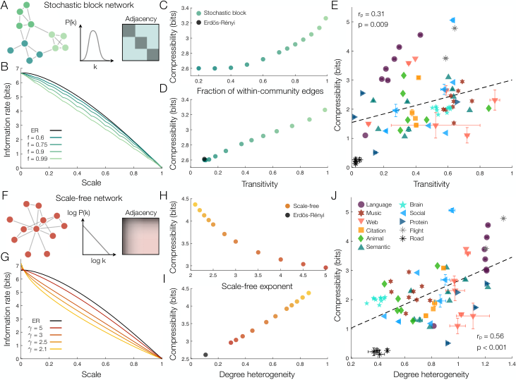
Based on the properties of optimal compressions (Fig. 4), we hypothesized that the compressibility of a network should increase with both (i) transitivity and (ii) degree heterogeneity. These two features are frequently observed across an array of real-world networks, from social, scientific, and biological interactions Ravasz and Barabási 2003; Tomassini and Luthi 2007; Ravasz 2009 to the Internet Vázquez et al. 2002, language Ravasz and Barabási 2003, music Farbood et al. 2015, and the brain Bassett et al. 2008. Moreover, the combination of transitivity (with tightly-connected modules) and heterogeneous degrees (with well-connected hubs) defines hierarchical organization Ravasz and Barabási 2003, which has been shown to support multi-scale representations of complex networks Sales-Pardo et al. 2007; Rosvall and Bergstrom 2011 and enable efficient information processing in neural and communication systems Bassett et al. 2010; Lynn et al. 2020. In fact, when encoding information about the world, the brain itself often employs hierarchical representations Balaguer et al. 2016; Diaconescu et al. 2014; Friston 2008. If correct, our hypotheses will lend to these perspectives a new outlook on the role of hierarchical structure: that it supports the efficient compression of complex networks.
To investigate the impact of transitivity and modular structure on compressibility, we consider a class of stochastic block networks (Fig. 5A), wherein nodes are grouped into modules of equal size and a specified fraction of the edges in the network connect nodes within the same module. We find that optimal compressions take advantage of this modular structure by clustering together nodes within the same module (see Supporting Fig. 3). Indeed, strengthening the modular structure – that is, increasing the fraction of within-module edges – decreases the rate-distortion curve (Fig. 5B). We therefore find that compressibility increases with both modularity (Fig. 5C) and transitivity (Fig. 5D). Importantly, these results on stochastic block networks generalize to real networks, with increases in transitivity yielding significant improvements in network compressibility (Fig. 5E).
To examine the dependence of compressibility on degree heterogeneity, we study scale-free networks (Fig. 5F), which have heavy-tailed degree distributions characterized by a power-law exponent Barabási and Albert 1999. Optimal compressions exploit this heterogeneous structure by clustering together high-degree hub nodes (see Supporting Fig. 3). As decreases, accentuating the heterogeneity in node degrees, the rate-distortion curve increases at small scales and decreases at intermediate and large scales (Fig. 5G). Both of these rate-distortion effects serve to improve the compressibility of scale-free networks (Fig. 5H). Moreover, rather than indirectly investigating the impact of heavy-tailed structure via the scale-free exponent , we can directly quantify the degree heterogeneity of a given network , where is the absolute difference in degrees averaged over all pairs of nodes and is the average degree. We find that the compressibility of scale-free networks grows linearly with degree heterogeneity (Fig. 5I), a result that generalizes to real networks (Fig. 5J). Furthermore, we confirm that the dependencies of compressibility on both transitivity and degree heterogeneity extend to directed networks (Supporting Fig. 5) and are robust to our choice of clustering heuristics (Supporting Fig. 6).
Together, the above results demonstrate that transitivity and degree heterogeneity – the two defining features of hierarchical organization – increase the compressibility of complex networks. Indeed, in networks with explicit hierarchical organization (such as those examined in Ref. Ravasz and Barabási 2003), we verify that optimal compressions capitalize on both modular structure and heterogeneous degrees in order to reduce the information rate (see Supporting Fig. 3). By contrast, for networks with uniform structure (such as Erdös-Rényi or -regular networks), natural groupings of nodes do not exist (see Supporting Fig. 3), and therefore such networks are highly incompressible (Fig. 5D,I).
Interestingly, by focusing on specific families of networks, we discover variations in compressibility that reflect a network’s specific function. Road networks, for example, exhibit the lowest transitivity and degree heterogeneity, and therefore the lowest compressibility, among the networks studied. This low compressibility is likely due to the fact that, unlike the other networks, road networks are confined to exist in two dimensions, severely constraining their topology Sperry et al. 2017. Besides road networks, we find that protein interactions have the lowest transitivity and brain networks have the lowest degree heterogeneity, leading both classes of networks to be relatively incompressible. Interestingly, these two families are unique among the networks studied in that they are only encoded genetically and need not be represented cognitively by a human or animal. By contrast, language networks are highly compressible, perhaps reflecting the primary function of language as a means for encoding and communicating information. Thus, although many networks are encoded biologically, the pressure for these encodings to be efficient manifests to varying degrees in different families of networks, yielding a spectrum of compressibilities.
Discussion
Complex networks perform an astonishing array of functions, which are supported by a multitude of topological structures. Many networks, however, are unified by a common constraint: that they rely on biological entities to encode them and pass them on. Encoding a network efficiently – that is, striking an optimal balance between simplicity and accuracy – requires compression, an insight that has provided information-theoretic perspectives on network structure Rosvall and Bergstrom 2008; Rosvall and Bergstrom 2007; Slonim et al. 2005. Naturally, some networks should be more compressible than others, with structural regularities enabling efficient representations across multiple scales. To investigate this hypothesis, here we introduce a rate-distortion theory of network compression (Fig. Compressing random walks) and propose a quantitative definition for the compressibility of a network (Eq. 2; Fig. 2A). Applying our framework to a number of real and model networks, we demonstrate that network compressibility increases with both transitivity and degree heterogeneity (Fig. 5), two features that together characterize hierarchical organization Ravasz and Barabási 2003.
The interplay between network structure and compressibility hints at one possible factor contributing to the hierarchical organization observed in many real networks Ravasz and Barabási 2003; Sales-Pardo et al. 2007; Ravasz et al. 2002; Dodds et al. 2003; Bassett et al. 2010; Lynn et al. 2020; Farbood et al. 2015; Vázquez et al. 2002; Bassett et al. 2008; Tomassini and Luthi 2007; Ravasz 2009: that it enables efficient representations across scales. But do the actual encodings themselves – from representations in the minds of humans and animals to the information stored in the genetic code – take advantage of this hierarchical organization? Moreover, do the encodings employed in nature approach the limit of optimal efficiency specified by rate-distortion theory? Answering these questions will require new exciting investigations into the information-theoretic forces that shape complex networks.
Entropy of random walks
Given a (possibly weighted, directed) network with adjacency matrix , the probability of one node transitioning to another node in a random walk is , where is the (out) degree of node (Fig. Compressing random walksA). The entropy of random walks is given by
| (5) |
where is the stationary distribution defined by the condition (which we note is uniquely defined if the network is strongly-connected and aperiodic). For undirected networks, Eq. 5 simplifies significantly. In this case, the stationary distribution is proportional to the node degrees , where is the number of edges in the network, and thus the entropy takes the form
| (6) |
If, in addition, the nodes have uniform degree (as in the -regular networks in Fig. 2) then the entropy equals . For example, in the simple network in Fig. Compressing random walks, the nodes have uniform degree 4, and thus the entropy is 2 bits.
Bounding the information rate
After clustering a network, a random walk gives rise to a new sequence , where is the cluster containing node (Fig. Compressing random walksB). The information rate of this sequence is given by the mutual information , which for deterministic clusterings (such as those considered here) is equivalent to the entropy . However, even though the random walk is Markovian (yielding a simple form for the entropy (Eq. 5)), the clustered sequence need not be Cover and Thomas 2012, and thus it is generally difficult to derive an analytic form for .
Despite this hurdle, there exist simple bounds on the information rate , summarized by the inequalities
| (7) |
where and are the conditional entropies of on and , respectively Cover and Thomas 2012. These bounds are tight at the minimum scale , when each cluster contains one node and so . The bounds are also tight at the maximum scale , when there is one cluster and so .
To compute the lower bound at intermediate scales, we begin with the conditional probability of node in the random walk transitioning to cluster in the clustered sequence , . Then, the lower bound is given by
| (8) |
where the second sum runs over all clusters . Similarly, to compute the upper bound, we consider the probability of one cluster transitioning to another cluster ,
| (9) |
where is the stationary distribution over clusters. We then arrive at the following upper bound,
| (10) |
which is exact if the clustered sequence is Markovian. In practice, when estimating the optimal information rate for a network, we minimize the upper bound in Eq. 10 over clusterings, resulting in an upper bound on the rate-distortion curve.
The upper bound simplifies significantly for unweighted, undirected networks. In this case, the cluster transition probabilities take the form , where is the induced network of clusters and is the sum of the degrees of the nodes in . Recalling that the stationary distribution simplifies to , one can manipulate Eq. 10 into the form
| (11) |
Under the further simplification of a clustering with one large cluster and minimal clusters of one node each (Fig. 4), this upper bound can be fashioned into Eq. 1.
Clustering algorithm
To compute the rate-distortion curve , we use an agglomerative clustering algorithm. Beginning with clusters (corresponding to the minimum scale ), each containing an individual node, we iteratively combine pairs of clusters until we eventually arrive at one large cluster containing the entire network (corresponding to the maximum scale ). At each step, we greedily select the pair of clusters to combine that minimizes the information rate (Eq. 10). However, rather than searching through all pairs of clusters at each iteration (which would limit applications to small networks), we instead focus on a subset of pairs chosen through one of two heuristics.
The first heuristic, motivated by the observation that optimal clusterings tend to combine clusters with large degrees (Fig. 4E), selects the pairs of clusters and with the largest combined stationary probabilities . For unweighted, undirected networks, we note that this choice is equivalent to selecting the pairs of clusters with the largest combined degrees, since . The second heuristic, motivated by the fact that optimal compressions tend to form clusters with tight intra-cluster connectivity (Fig. 4D), selects the pairs of clusters and with the largest combined joint transition probabilities . For unweighted, undirected networks, we remark that this second heuristic is equivalent to selecting the pairs of clusters with the largest number of connecting edges, since . In practice, we consider pairs of clusters at each iteration. In Supporting Fig. 1, we compare these two heuristics to the brute-force approach that searches through all pairs of clusters at each iteration of the clustering algorithm. In addition to significantly speeding up the algorithm, we find that these two heuristics often yield more accurate estimates of the rate-distortion curve than the brute-force implementation.
Network datasets
The networks analyzed in this paper are listed and described in Supporting Table 1. While we study unweighted, undirected versions of the networks in Figs. 4, 2E, 5E, and 5J, similar results hold for directed versions of the networks (Supporting Figs. 2 and 3). For networks of size , we perform analyses directly. For larger networks with , we analyze 50 subnetworks of nodes each. Each subnetwork is generated by performing a random walk beginning at a randomly-selected node until nodes have been reached. This sampling method has been shown to give accurate estimates of network statistics Leskovec and Faloutsos 2006.
Data and code availability
The data analyzed in this paper and the code used to perform the analyses are openly available at github.com/ChrisWLynn/Network_compressibility.
The authors thank Christopher Kroninger, Lia Papadopoulos, Dr. Pragya Srivastava, Mathieu Ouellet, and Dale Zhou for helpful feedback on earlier versions of this manuscript. C.W.L. acknowledges support from the James S. McDonnell Foundation 21 Century Science Initiative Understanding Dynamic and Multi-scale Systems - Postdoctoral Fellowship Award. The authors also acknowledge support from the John D. and Catherine T. MacArthur Foundation, the ISI Foundation, the Paul G. Allen Family Foundation, the Army Research Laboratory (W911NF-10-2-0022), the Army Research Office (Bassett-W911NF-14-1-0679, Falk-W911NF-18-1-0244, Grafton-W911NF-16-1-0474, DCIST- W911NF-17-2-0181), the Office of Naval Research, the National Institute of Mental Health (2-R01-DC-009209-11, R01-MH112847, R01-MH107235, R21-M MH-106799), and the National Science Foundation (NSF PHY-1554488, BCS-1631550, and NCS-FO-1926829).
CITATION DIVERSITY STATEMENT
Recent work in several fields of science has identified a bias in citation practices such that papers from women and other minorities are under-cited relative to the number of such papers in the field Mitchell et al. 2013; Dion et al. 2018; Caplar et al. 2017; Maliniak et al. 2013; Dworkin et al. 2020; Bertolero et al. 2020. Here we sought to proactively consider choosing references that reflect the diversity of the field in thought, form of contribution, gender, and other factors. We obtained predicted gender of the first and last author of each reference by using databases that store the probability of a name being carried by a woman Dworkin et al. 2020; Zhou et al. 2020. By this measure (and excluding self-citations to the first and last authors of our current paper), our references contain woman(first)/woman(last), man/woman, woman/man, and man/man. This method is limited in that a) names, pronouns, and social media profiles used to construct the databases may not, in every case, be indicative of gender identity, and b) it cannot account for intersex, non-binary, or transgender people. Second, we obtained predicted racial/ethnic category of the first and last author of each reference by databases that store the probability of a first and last name being carried by an author of color Ambekar et al. 2009; Sood and Laohaprapanon 2018. By this measure (and excluding self-citations), our references contain author of color(first)/author of color(last), white author/author of color, author of color/white author, and white author/white author. This method is limited in that a) names, Census entries, and Wikipedia profiles used to make the predictions may not be indicative of racial/ethnic identity, and b) it cannot account for Indigenous and mixed-race authors, or those who may face differential biases due to the ambiguous racialization or ethnicization of their names. We look forward to future work that could help us to better understand how to support equitable practices in science.
Supporting Information
1 Introduction
In this Supporting Information, we provide extended analysis and discussion to support the results presented in the main text. In Sec. 2, we discuss the information costs of the different edge types in Fig. 2C in the main text. In Sec. 3, we derive an analytic approximation of the rate-distortion curve for -regular networks (Eq. 3 and Fig. 3C in the main text). In Sec. 4, we discuss the different heuristics used to speed up the clustering algorithm and compare their estimates of optimal information rates with those of a brute-force implementation. In Sec. 5, we demonstrate that the tractable upper bound on the rate-distortion curve used throughout the main text provides a reasonable approximation to the true rate-distortion curve. In Sec. 6, we study the structure of optimal compressions for the model networks analyzed in the main text. In Sec. 7, we demonstrate that the central results from the main text generalize to directed networks. In Sec. 8, we show that the dependencies of compressibility on average degree, transitivity, and degree heterogeneity do not depend on the heuristics used to speed up the clustering algorithm. Finally, in Sec. 9, we list the real networks analyzed in this work and describe how we sample large networks.
2 Information content of different edges
When analyzing optimal clusterings (that is, clusterings that minimize the information rate , Eq. 9 in the main text), we find that they tend to consist of one large cluster containing nodes and clusters containing one node each (see Fig. 2A, B in the main text). This observation allows us to group the edges in a network into three categories (Fig. 2C in the main text): those connecting nodes within , those connecting nodes outside of , and those on the boundary of (connecting nodes within to nodes outside of ).
In order to predict the structure of the one large cluster , we wish to compare the contributions of different edge types to the information rate . For an unweighted, undirected network with adjacency matrix , and a clustering with one large cluster , the information rate can be written as
| (12) |
where the sums run over all nodes not in , is the number of edges in the network, is the degree of node , is the combined degrees of nodes in , is the number of edges connecting a node to nodes in , and is the number of edges connecting nodes within (see Materials and Methods in the main text).
Within versus boundary edges
If we add an edge between two nodes within , then both and increase by two, and the change in the information rate is given by
| (13) |
where the approximation follows by letting and . By contrast, adding an edge on the boundary of (say, connecting a node outside of to a node in ) yields a contribution to the information rate of
| (14) |
where the approximation follows from , , and .
It is clear that will be less than if . Given a random selection of nodes to include in , both the fraction of edges emanating from that end in and the fraction of edges emanating from that end in are approximated by the proportional size of ; namely, . Because , for a randomly-selected cluster we have . Thus, the information cost of edges within () is likely to be lower than the cost of an edge on the boundary of (), leading to the prediction that optimal clusters will seek to include tightly-knit communities with sparse connectivity to the rest of the network. We confirm this prediction in real networks (Fig. 2D in the main text), and we further demonstrate that modular structure and tight clustering serve to increase network compressibility (Fig. 4A-E in the main text).
Within versus outside edges
Now consider an edge connecting two nodes and outside of . Adding such an edge increases the information rate by an amount
| (15) |
where the approximation follows from and . Comparing Eqs. 2 and 2, we see that will be less than if . Based on the above result that optimal clusters tend to include tight within-cluster connectivity, we know that the proportion is greater than the scale (see Fig. 2D in the main text). Thus, we will have (and therefore ) across most scales (specifically, for all scales ). This result indicates that optimal clusters will seek to include high-degree nodes and exclude low-degree nodes, which we confirm in Fig. 2E in the main text. Moreover, because compression leverages differences in node degrees, we find that networks with heterogeneous (or heavy-tailed) degrees are highly compressible (Fig. 4F-J in the main text).
3 Rate-distortion curve for -regular networks
We wish to derive an analytic approximation to the rate-distortion curve for -regular networks (Fig. 3B in the main text). For unweighted, undirected networks and a clustering including one large cluster of size , the information rate is given in Eq. 2. Let us examine each term individually:
- •
The large cluster contains nodes, and so the number of nodes outside of is . Since each node in the network has degree , we have
(16) and
(17) - •
Assuming that each edge has a probability of connecting to nodes in , we can approximate and . Thus, we can approximate
(18) and
(19)
Plugging Eqs. 16-19 into Eq. 2, and noting that , after some algebra we arrive at an analytic approximation to the rate-distortion curve for a -regular network,
| (20) |
We demonstrate that this prediction provides a good approximation to true rate-distortion curves, and becomes accurate in the high-degree limit (Fig. 3C in the main text).
4 Speeding up the clustering algorithm
To compute the rate-distortion curve for a given network, one must identify clusterings that minimize the information rate across all scales (equivalently, for all numbers of clusters ). Here, we employ a greedy clustering algorithm that iteratively combines pairs of clusters so as to minimize the information rate (see Materials and Methods in the main text). Specifically, beginning with clusters (one for each node in the network), we attempt to combine different pairs of clusters and compute the resulting changes to the information rate . Combining the pair of clusters that yields the largest reduction in information rate, we arrive at a new clustering with clusters. Repeating this process for all numbers of clusters , we arrive at estimates of the optimal clusterings and information rates across all scales .
A brute force implementation of this algorithm would attempt to combine all pairs of clusters at each iteration. For each pair of clusters, one would then compute the new information rate
| (21) |
where is the stationary distribution over clusters, and
| (22) |
is the conditional probability of transitioning from cluster to cluster . Since Eq. 21 involves summing over all pairs of clusters and , computing the information rate requires computations. Finally, the algorithm repeats this process for all numbers of clusters , requiring a total of computations. This dependence limits a naïve implementation of our clustering algorithm to small networks. In what follows, we will show how to reduce this size dependence to , significantly improving the efficiency of the algorithm and enabling applications to networks of reasonable size.
Change in information rate
As discussed above, a naïve implementation of the algorithm would re-compute the information rate (Eq. 21) after attempting to combine each pair of clusters, requiring computations. However, we only require the change in the information rate, a computation that we will see takes time.
Consider attempting to combine two clusters and . Before combining the clusters, the information rate is given by
| (23) |
After combining the clusters and , the new information rate is given by
| (24) |
Thus, the change in the information after combining clusters and is given by
| (25) |
Although Eq. 4 appears more complicated than Eq. 21, we remark that it only requires summing over the different clusters rather than all pairs of clusters and . Therefore, by computing the change in information rate rather than the information rate itself, we reduce the number of computations from to .
Heuristics for cluster selection
In the naïve implementation of the clustering algorithm, one searches through all pairs of clusters at each iteration to find the pair whose combination yields the largest decrease in the information rate. Here, we instead propose two heuristics for selecting a subset of pairs of clusters at each iteration, thereby reducing the number of pairs from to . For all results here and in the main text, we consider pairs of clusters at each iteration of the clustering algorithm.
The first heuristic is motivated by the observation that optimal clusterings tend to include one large cluster with high-degree nodes (Fig. 2E in the main text). In undirected networks, the stationary distribution over clusters is proportional to the cluster degrees, such that , where is the degree of cluster and is the number of edges in the network. We therefore select the pairs of clusters and with the largest combined stationary probabilities ; for undirected networks, this process is equivalent to selecting the pairs of clusters with the largest combined degrees .
The second heuristic is motivated by the observation that the one large cluster tends to include nodes that are tightly connected to one another (Fig. 2D in the main text). In undirected networks, the joint transition probability from one cluster to another is proportional to the number of edges between the clusters, such that , where is the number of edges connecting nodes in to nodes in . We therefore select the pairs of clusters and with the largest joint transition probabilities ; for undirected networks, this process is equivalent to selecting the pairs of clusters with the largest number of connecting edges .
To evaluate the performance of these two heuristics, we compare the rate-distortion curves for the real networks in Supporting Table 1 computed using (i) the brute-force approach that attempts to combine all pairs of clusters, (ii) the stationary distribution heuristic, and (iii) the joint transition probability heuristic. Since each algorithm computes an upper bound on the rate-distortion curve for a given network, whichever algorithm returns a smaller upper bound will have achieved a more accurate estimate of the true rate-distortion curve . Consider, for example, the social network of bottlenose dolphins Lusseau et al. 2003. For scales , we find that the stationary distribution heuristic provides a lower (and thus more accurate) upper bound on the rate-distortion curve than both the brute-force algorithm and the joint transition probability heuristic (Supporting Fig. 1A). By contrast, for scales , the joint transition probability heuristic provides the most accurate estimate of the rate-distortion curve (Supporting Fig. 1A). Notably, even though both heuristics only consider a limited set of cluster pairs, they both produce rate-distortion estimates that are comparable in accuracy to, if not more accurate than, the brute-force approach that searches through all pairs at each iteration.
To compare the accuracy of the different algorithms (that is, to determine which algorithm provides a lower upper bound across all scales) we can compare their compressibility estimates,
| (26) |
If one algorithm produces a lower (that is, more accurate) rate-distortion estimate on average across all scales , then one will arrive at a larger lower bound on the compressibility . In Supporting Fig. 1B, we see that the compressibility computed using the stationary distribution heuristic is almost always as large as (if not larger than) that computed using all pairs of clusters for the real networks in Supporting Table 1. Similarly, in Supporting Fig. 1C we see the joint transition probability heuristic provides compressibility estimates that are nearly as accurate as across most of the real networks. In fact, the brute-force compressibility estimates are significantly larger (that is, more accurate) than both of the heuristic estimates and for only 10 of the 69 real networks.
Together, these results demonstrate that the two cluster-selection heuristics provide rate-distortion estimates that are comparable, if not more accurate, than the brute-force clustering algorithm. Moreover, these heuristics reduce the search for an optimal pair of clusters at each iteration from pairs to pairs. In combination with the speed-up in Sec. 4, this reduces the total run-time of the clustering algorithm from to , thereby allowing applications to networks of reasonable size.
5 Errors in information bounds
In the main text, rather than computing the information rate of a given clustering directly, we instead consider a tractable upper bound (see Materials and Methods in the main text). For a given network, we minimize across all scales to arrive at an upper bound on the rate-distortion curve , which we then use to compute a lower bound on the compressibility (Eq. 2). The upper bound on the rate-distortion curve and the corresponding lower bound on the compressibility together form the basis of our main results (Figs. 3 and 4 in the main text). Therefore, it is important to verify that these bounds provide reasonable approximations to the true rate-distortion curves and compressibilities of the networks analyzed in the main text.
To investigate the accuracy of the upper bound on the rate-distortion curve , we consider a tractable lower bound (see Materials and Methods in the main text). Importantly, the true rate-distortion curve lies between the upper and lower bounds, such that . Thus, the error in the upper bound () is no larger than the difference between the upper and lower bounds (). Put simply, if the difference between the bounds is small, then we know that the error is even smaller.
For all networks, one can show that the upper and lower bounds are equal (and therefore exact) at both the minimum scale and the maximum scale (see Materials and Methods in the main text). Moreover, in the main text, we demonstrated for Zachary’s karate club Zachary 1977 that the upper bound remains close to the lower bound across all intermediate scales (Fig. 2A in the main text). In order to compare the rate-distortion bounds across different networks, here we normalize and by the entropy of each network. Notably, we find that a tight correspondence between the upper and lower bounds is not unique to Zachary’s karate club, but instead is a general feature of the real networks in Supporting Table 1 (Supporting Fig. 2A). Indeed, the maximum difference between the upper and lower bounds tends to only reach about 10% of the entropy of a network (Supporting Fig. 2B). For comparison, the difference between bounds is actually larger in Zachary’s karate club (reaching 15% of the entropy) than the typical network in Supporting Table 1 (Supporting Fig. 2B). These results establish that the upper bound provides a good approximation to the true rate-distortion curve .
We now investigate the accuracy of the lower bound on the compressibility (Eq. 2). To do so, we consider the upper bound on the compressibility induced by the lower bound on the rate-distortion curve. We find that the lower bound remains close to the upper bound across almost all networks in Supporting Table 1 (Supporting Fig. 2C). For comparison, Zachary’s karate club exhibits a difference that is typical for the networks in Supporting Table 1 (Supporting Fig. 2C, right). Interestingly, among the five outliers with an abnormally large difference , four are the road networks in Supporting Table 1 (Supporting Fig. 2C, right). As discussed in the main text, the abnormal compression properties of road networks likely reflects the unique physical constraints on their structure. Together, the results of this section verify that the upper bound on the rate-distortion curve and the corresponding lower bound on the compressibility provide reasonable estimates of the true information properties of the real networks analyzed in the main text.
6 Compressing model networks
In our investigations of network compressibility, we analyzed a number of model networks, including Erdös-Rényi, -regular (Fig. 3B in the main text), stochastic block (Fig. 4A in the main text), and scale-free (Fig. 4F in the main text) networks. Here, we study the structure of optimal compressions in these model networks, as well as networks with hierarchical structure, wherein small tightly-connected groups of nodes connect to form larger, but looser groups Ravasz and Barabási 2003.
To recall, based on the information content of different edges (see Sec. 2), we predicted that optimal compressions would tend to maximize the number of edges within the one large cluster and minimize the number of edges on the boundary and outside of the cluster. In the main text, we confirmed these predictions for the real networks in Supporting Table 1 (see Fig. 2 in the main text). In Supporting Fig. 3, we verify that these results extend to all of the model networks listed above.
First, across all model networks considered, we find that the edges emanating from the one large cluster tend to connect to nodes within the cluster (Supporting Fig. 3A) and avoid crossing over to nodes outside of the cluster (Supporting Fig. 3B). Interestingly, we observe stark differences in the properties of optimal compressions between different network models. For example, although Erdös-Rényi and -regular networks do not contain large-scale structure, optimal compressions are still able to identify groups of nodes that are slightly more strongly connected to each other than to the rest of the network. Meanwhile, optimal compressions in stochastic block, scale-free, and hierarchical networks identify groups of nodes with much stronger within-group connectivity. In fact, for stochastic block networks, it is clear that optimal compressions identify the built-in modules, with the one large cluster iteratively enveloping each module one by one as the scale increases (Supporting Fig. 3A-B).
Second, for Erdös-Rényi, scale-free, and hierarchical networks, we confirm that optimal compressions select groups of nodes with higher degrees than average (Supporting Fig. 3C) while omitting low-degree nodes (Supporting Fig. 3D). As expected, this effect is much stronger in scale-free and hierarchical networks (which exhibit large heterogeneities in node degree) than in Erdös-Rényi networks (which do not contain large-scale structure). We remark that in -regular networks, there are no differences in node degrees by definition. Similarly, for stochastic block networks, we find a negligible difference between the degrees of nodes inside versus outside the large cluster. This final result once again suggests that optimal compressions in stochastic block networks focus on their modular, rather than heterogeneous, structure. Together, the results of this section demonstrate that the structure of optimal compressions observed in real networks (Fig. 2 in the main text) extends to a range of model networks. Moreover, for hierarchical networks, we establish that optimal compressions cluster together groups of nodes that are more tightly connected than scale-free networks (Supporting Fig. 3A), yet higher in degree than stochastic block networks (Supporting Fig. 3C), thereby capitalizing on both the modular and heterogeneous properties of hierarchical organization.
7 Directed networks
In the main text, in order to develop analytic predictions for the structure of optimal clusterings and the impact of network structure on compressibility, we focused on the special case of undirected networks. Specifically, we predicted (and confirmed) that optimal compressions would tend to maximize the number of edges within the one large cluster and minimize the number of edges on the boundary and outside of the cluster (Fig. 2D-E in the main text). In turn, these findings led to the predictions that network compressibility (Eq. 26) should increase with both modular structure and heavy-tailed degrees, which we confirmed in undirected real and model networks (Fig. 4 in the main text). Here we demonstrate that these central results from the main text are not limited to undirected networks, but in fact generalize to directed networks.
Structure of optimal compressions
Our clustering algorithm described in the main text is general, applying to any weighted, directed network. We can therefore use the algorithm to compute optimal compressions and rate-distortion curves for the directed real networks listed in Supporting Table 1. We remark that among the 69 real networks studied in the main text, 38 have directed versions (see Supporting Table 1), which we analyze here.
As was the case for undirected networks (Fig. 2B in the main text), we find that optimal compressions in directed networks tend to form one large cluster with the maximum possible size , where is the scale of description, and minimal clusters containing one node each (Supporting Fig. 4A). To analyze the structure of the large cluster, in the main text we divided the edges in an undirected network into three categories (Fig. 2C in the main text): those within the cluster, those outside of the cluster, and those on the cluster boundary. For directed networks, we can further divide boundary edges into two categories – those connecting from inside to outside the cluster and those connecting from outside to inside the cluster – thereby resulting in a total of four edge types (Supporting Fig. 4B).
For undirected networks, in the main text we demonstrated that the one large cluster had tight within-cluster connectivity (maximizing the number of edges inside the cluster) and sparse connectivity to the rest of the network (minimizing the number of boundary edges; Fig. 2D in the main text). Indeed, this result generalizes to directed networks, with the one large cluster favoring within-cluster edges over both outgoing (Supporting Fig. 4C) and incoming (Supporting Fig. 4D) boundary edges. In the main text, we also demonstrated that the one large cluster sought to include high-degree nodes and exclude low-degree nodes in undirected networks (Fig. 2E in the main text). Here, we confirm that this result also applies to directed networks, with the one large cluster containing nodes with both larger out-degrees (Supporting Fig. 4E) and in-degrees (Supporting Fig. 4F) than the rest of the network. Together, these results establish that our predictions about the structure of optimal compressions (see Sec. 2) generalize to directed networks.
Impact of network structure on compressibility
We are now prepared to study the compressibility of directed networks. In the main text, we demonstrated that the compressibility of undirected networks increases with the logarithm of the average degree (Fig. 3E in the main text). Moreover, based on the structure of optimal clusterings (Fig. 2 in the main text), we hypothesized (and confirmed) that the compressibility of undirected networks increases with both transitivity and degree heterogeneity (Fig. 4 in the main text). Here, we demonstrate that each of these results about the impact of network structure on compressibility generalizes to directed networks.
We begin by analyzing the dependence of network compressibility on average degree. For a directed network with adjacency matrix , where if there is a directed edge from node to node , the out-(in-)degree of node is given by (). Despite each node possibly having different out- and in-degrees, the average out- and in-degrees in a network are equal, since
| (27) |
Therefore, even for directed networks, we can simply discuss the average degree. In Supporting Fig. 5A, we demonstrate that the compressibility (Eq. 26) of real directed networks grows logarithmically with the average degree, confirming that our prediction for undirected networks (Fig. 3D-E in the main text) extends to directed networks.
We now consider the impact of transitivity on the compressibility of directed networks. As in the main text, we quantify transitivity using the average clustering coefficient. For undirected networks, the clustering coefficient of a node is the number of edges connecting the neighbors of divided by the possible connections, and the average clustering coefficient is given by averaging over the nodes in a network. Although the clustering coefficient was originally defined for undirected networks, this definition has since been extended to directed networks Fagiolo 2007. In a directed network, the clustering coefficient of a node is the number of connected pairs among its out- and in-neighbors divided by the possible connections. Just as we found for undirected networks (Fig. 4A-E in the main text), the compressibility of directed networks is significantly correlated with the average clustering coefficient (Supporting Fig. 5B), thereby indicating that transitivity and the presence of tightly-knit communities serve to make networks more compressible.
Finally, we study the impact of heterogeneous (or heavy-tailed) degrees on the compressibility of directed networks. For directed networks, there are two definitions of degree heterogeneity: that of out-degrees and that of in-degrees . We find that the compressibility of directed networks is significantly correlated with both the out-degree (Supporting Fig. 5C) and in-degree (Supporting Fig. 5D) heterogeneities. Thus, even in directed networks, heavy-tailed degree distributions with well-connected hubs serve to increase network compressibility. Together, these results demonstrate that the central conclusions from the main text generalize to directed networks; namely, that strong transitivity and degree heterogeneity – the two defining features of hierarchical organization Ravasz and Barabási 2003 – increase the compressibility of complex networks.
8 Robustness to clustering heuristics
In the main text, we computed rate-distortion curves using our clustering algorithm with the pair-selection heuristics described in Sec. 4. We found that network compressibility increased with average degree (Fig. 3D-E in the main text), transitivity (quantified by average clustering coefficient; Fig. 4D-E in the main text), and degree heterogeneity (Fig. 4I-J in the main text). Here, we confirm that these results are not simply due to our choices of clustering heuristics. To do so, we recompute the compressibilities of the networks in Supporting Table 1 using the brute-force implementation of our clustering algorithm that searches through all pairs of clusters at each iteration (see Sec. 4). We remark that, in order to employ the brute-force implementation, for each network of size we analyze 50 randomly-sampled subnetworks of 100 nodes each. Using the brute-force algorithm, we confirm that the compressibility increases with average degree (Supporting Fig. 6A), transitivity (Supporting Fig. 6B), and degree heterogeneity (Supporting Fig. 6C). These observations demonstrate that the central results from the main text are robust to our choice of pair-selection heuristic in the clustering algorithm.
9 Network datasets and processing
The real-world networks analyzed in the main text are listed and briefly described in Supporting Table 1. The web, citation, animal, semantic, social, protein, flight, and road networks are gathered from online network repositories. The language and music networks were generated by the authors previously (see below) Lynn et al. 2020. The brain networks are generated from structural and functional data gathered and analyzed previously (see below)Van Essen et al. 2013; Bertolero and Bassett 2020.
For the language networks, we developed code to (i) remove punctuation and white space, (ii) filter words by their part of speech, and (iii) record the transitions between the filtered words Lynn et al. 2020. Here we focus on networks of transitions between nouns, noting that the same methods can be used to record transitions between other parts of speech. The raw text was gathered from Project Gutenberg (gutenberg.org/wiki/Main_Page).
| Type | Name | Description | Reference | ||
| Language | Shakespeare: Combined works∗ | 11,234 | 97,892 | Noun transitions. | Shakespeare 2007 |
| Homer: Iliad∗ | 3,556 | 23,608 | Noun transitions. | Pope et al. 1891 | |
| Plato: Republic∗ | 2,271 | 9,796 | Noun transitions. | Jowett 1888 | |
| Jane Austen: Pride and Prejudice∗ | 1,994 | 12,120 | Noun transitions. | Austen 2001 | |
| William Blake: Songs of Innocence…∗ | 370 | 781 | Noun transitions. | Blake 1998 | |
| Miguel de Cervantes: Don Quixote∗ | 6,090 | 43,682 | Noun transitions. | Cervantes 2018 | |
| Walt Whitman: Leaves of Grass∗ | 4,791 | 16,526 | Noun transitions. | Whitman 2017 | |
| Music | Michael Jackson: Thriller∗ | 67 | 446 | Note transitions. | Jackson 1984 |
| Beatles: Hard Day’s Night∗ | 41 | 212 | Note transitions. | The Beatles 1964 | |
| Queen: Bohemian Rhapsody∗ | 71 | 961 | Note transitions. | Queen 1975 | |
| Toto: Africa∗ | 39 | 163 | Note transitions. | Toto 1982 | |
| Mozart: Sonata No 11∗ | 55 | 354 | Note transitions. | Mozart 1784 | |
| Beethoven: Sonata No 23∗ | 69 | 900 | Note transitions. | Beethoven 1807 | |
| Chopin: Nocturne Op 9-2∗ | 59 | 303 | Note transitions. | Chopin 1832 | |
| Bach: Clavier Fugue 13∗ | 40 | 143 | Note transitions. | Bach 1722 | |
| Brahms: Ballade Op 10-1∗ | 69 | 670 | Note transitions. | Brahms 1854 | |
| Web | Google internal∗ | 12,354 | 142,296 | Hyperlinks between internal Google cites. | Palla et al. 2007; Kunegis 2013 |
| Education | 2,622 | 6,065 | Hyperlinks between education webpages. | Gleich et al. 2004; Rossi and Ahmed 2015 | |
| EPA | 2,232 | 6,876 | Hyperlinks between pages linking to www.epa.gov. | De Nooy et al. 2011; Rossi and Ahmed 2015 | |
| Indochina | 9,638 | 45,886 | Hyperlinks between pages in Indochina. | Boldi et al. 2004; Rossi and Ahmed 2015 | |
| 2004 Election blogs∗ | 793 | 13,484 | Hyperlinks between blogs on US politics. | Adamic and Glance 2005; Kunegis 2013 | |
| Spam | 3,796 | 36,404 | Hyperlinks between spam pages. | Castillo et al. 2008; Rossi and Ahmed 2015 | |
| WebBase | 6,843 | 16,374 | Hyperlinks gathered by web crawler. | Boldi et al. 2004; Rossi and Ahmed 2015 | |
| Citation | arXiv Hep-Ph∗ | 12,711 | 139,500 | Citations in Hep-Ph section of the arXiv. | Leskovec et al. 2007; Kunegis 2013 |
| arXiv Hep-Th∗ | 7,464 | 115,932 | Citations in Hep-Th section of the arXiv. | Leskovec et al. 2007; Kunegis 2013 | |
| Cora∗ | 3,991 | 16,621 | Citations between scientific papers. | Šubelj and Bajec 2013; Kunegis 2013 | |
| DBLP∗ | 240 | 858 | Citations between scientific papers. | Ley 2002; Kunegis 2013 | |
| Animal | Dolphins | 62 | 159 | Social relationships. | Lusseau et al. 2003; Kunegis 2013 |
| Little Rock Lake | 183 | 2,434 | Food web of animal consumption. | Martinez 1991; Kunegis 2013 | |
| Macaques | 62 | 325 | Dominance relationships. | Takahata 1991; Kunegis 2013 | |
| Sheep | 24 | 91 | Dominance relationships. | Hass 1991; Kunegis 2013 | |
| Wetlands∗ | 128 | 2,075 | Food web of animal consumption. | Ulanowicz and DeAngelis 1999; Kunegis 2013 | |
| Zebras | 23 | 105 | Social interactions. | Sundaresan et al. 2007; Kunegis 2013 | |
| Semantic | Game of Thrones | 796 | 2,823 | Character co-occurrences. | Kunegis 2013 |
| Algebra | 278 | 3,553 | Concept co-occurrences. | Christianson et al. 2020 | |
| Bible | 1,707 | 9,059 | Pronoun co-occurrences. | Kunegis 2013 | |
| Les Miserables | 77 | 254 | Character co-occurrences. | Kunegis 2013 | |
| Edinburgh Thesaurus∗ | 7,754 | 226,518 | Word similarities in human experiments. | Kiss et al. 1973; Batagelj and Mrvar 2006 | |
| Roget Thesaurus∗ | 904 | 3,447 | Linked semantic categories. | Roget 1911; Batagelj and Mrvar 2006 | |
| Glossary terms | 60 | 114 | Words used in definitions of other words. | Batagelj and Mrvar 2006 | |
| FOLDOC∗ | 13,274 | 90,736 | Same as above (computing terms). | Howe 1993; Batagelj and Mrvar 2006 | |
| ODLIS∗ | 1,802 | 12,378 | Same as above (information science terms). | Reitz 2010; Batagelj and Mrvar 2006 | |
| Brain | Structural connectivity 1∗ | 100 | 806 | Structural connections between brain regions. | Van Essen et al. 2013 |
| Structural connectivity 2∗ | 100 | 858 | Structural connections between brain regions. | Van Essen et al. 2013 | |
| Structural connectivity 3∗ | 100 | 865 | Structural connections between brain regions. | Van Essen et al. 2013 | |
| Structural connectivity 4∗ | 100 | 916 | Structural connections between brain regions. | Van Essen et al. 2013 | |
| Structural connectivity 5∗ | 100 | 906 | Structural connections between brain regions. | Van Essen et al. 2013 | |
| Functional connectivity 1 | 100 | 811 | Functional correlations between brain regions. | Van Essen et al. 2013 | |
| Functional connectivity 2 | 100 | 800 | Functional correlations between brain regions. | Van Essen et al. 2013 | |
| Functional connectivity 3 | 100 | 830 | Functional correlations between brain regions. | Van Essen et al. 2013 | |
| Functional connectivity 4 | 100 | 854 | Functional correlations between brain regions. | Van Essen et al. 2013 | |
| Functional connectivity 5 | 100 | 799 | Functional correlations between brain regions. | Van Essen et al. 2013 | |
| Social | Zachary’s karate club | 34 | 78 | Interactions between karate club members. | Zachary 1977; Kunegis 2013 |
| 13,130 | 75,562 | Subset of the Facebook network. | Viswanath et al. 2009; Kunegis 2013 | ||
| arXiv Astr-Ph | 17,903 | 196,972 | Coauthorships in Astr-Ph section of arXiv. | Leskovec et al. 2007; Kunegis 2013 | |
| arXiv Hep-Th | 22,721 | 2,672,975 | Coauthorships in Hep-Th section of arXiv. | Leskovec et al. 2007; Kunegis 2013 | |
| Adolescent health∗ | 2,155 | 8,970 | Friendships between students. | Moody 2001; Kunegis 2013 | |
| Highschool∗ | 67 | 267 | Friendships between highschool students. | Coleman et al. 1964; Kunegis 2013 | |
| Jazz | 198 | 2,742 | Collaborations between jazz musicians. | Gleiser and Danon 2003; Kunegis 2013 | |
| Protein | C. elegans | 453 | 2,025 | Interactions between metabolites. | Duch and Arenas 2005; Kunegis 2013 |
| Human (Figeys) | 2,239 | 6,452 | Protein interactions. | Ewing et al. 2007; Kunegis 2013 | |
| Human (Stelzl)∗ | 1,706 | 6,207 | Protein interactions. | Stelzl et al. 2005; Kunegis 2013 | |
| Yeast | 1,870 | 2,277 | Protein interactions. | Jeong et al. 2001; Kunegis 2013 | |
| Flight | US Flights∗ | 1,574 | 28,236 | Flights between US airports. | Kunegis 2013 |
| OpenFlights∗ | 2,939 | 30,501 | Flights between world cities. | Opsahl et al. 2010; Kunegis 2013 |
| Type | Name | Description | Reference | ||
|---|---|---|---|---|---|
| Road | EuroRoad | 1,174 | 1,417 | Network of roads between European cities. | Šubelj and Bajec 2011; Kunegis 2013 |
| Chicago∗ | 12,982 | 39,018 | Network of roads in Chicago. | Eash et al. 1979; Kunegis 2013 | |
| New York City | 264,346 | 730,100 | Network of roads in New York. | Kunegis 2013 | |
| Bay Area | 321,270 | 794,830 | Network of roads in San Francisco area. | Kunegis 2013 |
For the music networks, we read in audio files in MIDI format using the readmidi function in MATLAB (R2018a). For each song, we split the notes by their channel, which represents the different instruments. For each channel, we created a network of note transitions. We then create a transition network representing the entire song by aggregating the transitions between notes across the different channels. The MIDI files were gathered from midiworld.com and from kunstderfuge.com. Our code and data are available upon request from the corresponding author.
For the brain networks, we study the structural and functional connectivity of five randomly-selected subjects from the Human Connectome Project Van Essen et al. 2013. For all subjects, the brain is divided into 100 predefined cortical regions Thomas Yeo et al. 2011. The structural connectivity networks reflect physical white-matter tracts between brain regions measured using diffusion tensor imaging (DTI). We threshold the structural networks to only include connections between regions that are stronger than the mean. The functional connectivity networks reflect Pearson correlations between regional brain activity. Specifically, the activity is defined by blood-oxygen-level-dependent (BOLD) functional magnetic resonance imagining (fMRI) signals. To ensure that the functional networks have approximately the same edge density as the structural networks, we threshold the functional networks to only include connections stronger than the mean plus one standard deviation.
References
- Sizemore et al. (2018) Ann E Sizemore, Elisabeth A Karuza, Chad Giusti, and Danielle S Bassett. Knowledge gaps in the early growth of semantic feature networks. Nat. Hum. Behav., 2(9):682, 2018.
- Vázquez et al. (2002) Alexei Vázquez, Romualdo Pastor-Satorras, and Alessandro Vespignani. Large-scale topological and dynamical properties of the Internet. Phys. Rev. E, 65(6):066130, 2002.
- Liu et al. (2010) Xiao Fan Liu, K Tse Chi, and Michael Small. Complex network structure of musical compositions: Algorithmic generation of appealing music. Physica A, 389(1):126–132, 2010.
- Girvan and Newman (2002) Michelle Girvan and Mark EJ Newman. Community structure in social and biological networks. Proc. Natl. Acad. Sci., 99(12):7821–7826, 2002.
- Brush et al. (2018) Eleanor R Brush, David C Krakauer, and Jessica C Flack. Conflicts of interest improve collective computation of adaptive social structures. Sci. Adv., 4(1):e1603311, 2018.
- Kalakoski and Saariluoma (2001) Virpi Kalakoski and Pertti Saariluoma. Taxi drivers’ exceptional memory of street names. Mem. Cogn., 29(4):634–638, 2001.
- Lynn and Bassett (2020) Christopher W Lynn and Danielle S Bassett. How humans learn and represent networks. In press, Proc. Natl. Acad. Sci. <arxiv.org/abs/1909.07186 >, 2020.
- Gavin et al. (2006) Anne-Claude Gavin, Patrick Aloy, Paola Grandi, Roland Krause, Markus Boesche, Martina Marzioch, Christina Rau, Lars Juhl Jensen, Sonja Bastuck, Birgit Dümpelfeld, et al. Proteome survey reveals modularity of the yeast cell machinery. Nature, 440(7084):631–636, 2006.
- Lynn and Bassett (2019) Christopher W Lynn and Danielle S Bassett. The physics of brain network structure, function and control. Nat. Rev. Phys., 1, 2019.
- Vértes et al. (2016) Petra E Vértes, Timothy Rittman, Kirstie J Whitaker, Rafael Romero-Garcia, František Váša, Manfred G Kitzbichler, Konrad Wagstyl, Peter Fonagy, Raymond J Dolan, Peter B Jones, et al. Gene transcription profiles associated with inter-modular hubs and connection distance in human functional magnetic resonance imaging networks. Philos. Trans. R. Soc. B, 371(1705):20150362, 2016.
- Whitaker et al. (2016) Kirstie J Whitaker, Petra E Vértes, Rafael Romero-Garcia, František Váša, Michael Moutoussis, Gita Prabhu, Nikolaus Weiskopf, Martina F Callaghan, Konrad Wagstyl, Timothy Rittman, et al. Adolescence is associated with genomically patterned consolidation of the hubs of the human brain connectome. Proc. Natl. Acad. Sci., 113(32):9105–9110, 2016.
- Shannon (1948) Claude E. Shannon. A mathematical theory of communication. Bell Syst. Tech. J., 27(3):379–423, 1948.
- Cover and Thomas (2012) Thomas M Cover and Joy A Thomas. Elements of information theory. John Wiley & Sons, 2012.
- Rosvall and Bergstrom (2008) Martin Rosvall and Carl T Bergstrom. Maps of random walks on complex networks reveal community structure. Proc. Natl. Acad. Sci., 105(4):1118–1123, 2008.
- Rosvall and Bergstrom (2007) Martin Rosvall and Carl T Bergstrom. An information-theoretic framework for resolving community structure in complex networks. Proc. Natl. Acad. Sci., 104(18):7327–7331, 2007.
- Slonim et al. (2005) Noam Slonim, Gurinder Singh Atwal, Gašper Tkačik, and William Bialek. Information-based clustering. Proc. Natl. Acad. Sci., 102(51):18297–18302, 2005.
- Leskovec et al. (2009) Jure Leskovec, Kevin J Lang, Anirban Dasgupta, and Michael W Mahoney. Community structure in large networks: Natural cluster sizes and the absence of large well-defined clusters. Internet Math., 6(1):29–123, 2009.
- Archer et al. (2013) Evan Archer, Il Memming Park, and Jonathan W Pillow. Bayesian and quasi-bayesian estimators for mutual information from discrete data. Entropy, 15(5):1738–1755, 2013.
- Zachary (1977) Wayne W Zachary. An information flow model for conflict and fission in small groups. J. Anthropol. Res., 33(4):452–473, 1977.
- Buluç et al. (2016) Aydın Buluç, Henning Meyerhenke, Ilya Safro, Peter Sanders, and Christian Schulz. Recent advances in graph partitioning. In Algorithm Engineering, pages 117–158. Springer, 2016.
- Newman and Reinert (2016) Mark EJ Newman and Gesine Reinert. Estimating the number of communities in a network. Phys. Rev. Lett., 117(7):078301, 2016.
- Benson et al. (2016) Austin R Benson, David F Gleich, and Jure Leskovec. Higher-order organization of complex networks. Science, 353(6295):163–166, 2016.
- Barabási and Albert (1999) Albert-László Barabási and Réka Albert. Emergence of scaling in random networks. Science, 286(5439):509–512, 1999.
- Goh et al. (2001) K-I Goh, Byungnam Kahng, and Doochul Kim. Universal behavior of load distribution in scale-free networks. Phys. Rev. Lett., 87(27):278701, 2001.
- Ravasz and Barabási (2003) Erzsébet Ravasz and Albert-László Barabási. Hierarchical organization in complex networks. Phys. Rev. E, 67(2):026112, 2003.
- Tomassini and Luthi (2007) Marco Tomassini and Leslie Luthi. Empirical analysis of the evolution of a scientific collaboration network. Physica A, 385(2):750–764, 2007.
- Ravasz (2009) Erzsébet Ravasz. Detecting hierarchical modularity in biological networks. In Computational Systems Biology, pages 145–160. Springer, 2009.
- Farbood et al. (2015) Morwaread M Farbood, David J Heeger, Gary Marcus, Uri Hasson, and Yulia Lerner. The neural processing of hierarchical structure in music and speech at different timescales. Front. Neurosci., 9:157, 2015.
- Bassett et al. (2008) Danielle S Bassett, Edward Bullmore, Beth A Verchinski, Venkata S Mattay, Daniel R Weinberger, and Andreas Meyer-Lindenberg. Hierarchical organization of human cortical networks in health and schizophrenia. J. Neurosci., 28(37):9239–9248, 2008.
- Sales-Pardo et al. (2007) Marta Sales-Pardo, Roger Guimera, André A Moreira, and Luís A Nunes Amaral. Extracting the hierarchical organization of complex systems. Proc. Natl. Acad. Sci., 104(39):15224–15229, 2007.
- Rosvall and Bergstrom (2011) Martin Rosvall and Carl T Bergstrom. Multilevel compression of random walks on networks reveals hierarchical organization in large integrated systems. PLoS One, 6(4):e18209, 2011.
- Bassett et al. (2010) Danielle S Bassett, Daniel L Greenfield, Andreas Meyer-Lindenberg, Daniel R Weinberger, Simon W Moore, and Edward T Bullmore. Efficient physical embedding of topologically complex information processing networks in brains and computer circuits. PLoS Comput. Biol., 6(4):e1000748, 2010.
- Lynn et al. (2020) Christopher W Lynn, Lia Papadopoulos, Ari E Kahn, and Danielle S Bassett. Human information processing in complex networks. Nat. Phys., pages 1–9, 2020.
- Balaguer et al. (2016) Jan Balaguer, Hugo Spiers, Demis Hassabis, and Christopher Summerfield. Neural mechanisms of hierarchical planning in a virtual subway network. Neuron, 90(4):893–903, 2016.
- Diaconescu et al. (2014) Andreea O Diaconescu, Christoph Mathys, Lilian AE Weber, Jean Daunizeau, Lars Kasper, Ekaterina I Lomakina, Ernst Fehr, and Klaas E Stephan. Inferring on the intentions of others by hierarchical bayesian learning. PLoS Comput. Biol., 10(9):e1003810, 2014.
- Friston (2008) Karl Friston. Hierarchical models in the brain. PLoS Comput. Biol., 4(11):e1000211, 2008.
- Sperry et al. (2017) Megan M Sperry, Qawi K Telesford, Florian Klimm, and Danielle S Bassett. Rentian scaling for the measurement of optimal embedding of complex networks into physical space. J. Complex Netw., 5(2):199–218, 2017.
- Ravasz et al. (2002) Erzsébet Ravasz, Anna Lisa Somera, Dale A Mongru, Zoltán N Oltvai, and A-L Barabási. Hierarchical organization of modularity in metabolic networks. Science, 297(5586):1551–1555, 2002.
- Dodds et al. (2003) Peter Sheridan Dodds, Duncan J Watts, and Charles F Sabel. Information exchange and the robustness of organizational networks. Proc. Natl. Acad. Sci., 100(21):12516–12521, 2003.
- Leskovec and Faloutsos (2006) Jure Leskovec and Christos Faloutsos. Sampling from large graphs. In Proceedings of the 12th ACM SIGKDD international conference on Knowledge discovery and data mining, pages 631–636, 2006.
- Mitchell et al. (2013) Sara McLaughlin Mitchell, Samantha Lange, and Holly Brus. Gendered citation patterns in international relations journals. Int. Stud. Perspect., 14(4):485–492, 2013.
- Dion et al. (2018) Michelle L Dion, Jane Lawrence Sumner, and Sara McLaughlin Mitchell. Gendered citation patterns across political science and social science methodology fields. Polit. Anal., 26(3):312–327, 2018.
- Caplar et al. (2017) Neven Caplar, Sandro Tacchella, and Simon Birrer. Quantitative evaluation of gender bias in astronomical publications from citation counts. Nat. Astron., 1(6):1–5, 2017.
- Maliniak et al. (2013) Daniel Maliniak, Ryan Powers, and Barbara F Walter. The gender citation gap in international relations. Int. Organ., 67(4):889–922, 2013.
- Dworkin et al. (2020) Jordan D Dworkin, Kristin A Linn, Erin G Teich, Perry Zurn, Russell T Shinohara, and Danielle S Bassett. The extent and drivers of gender imbalance in neuroscience reference lists. Nat Neurosci., 23(8):918–926, 2020.
- Bertolero et al. (2020) Maxwell A Bertolero, Jordan D Dworkin, Sophia U David, Claudia López Lloreda, Pragya Srivastava, Jennifer Stiso, Dale Zhou, Kafui Dzirasa, Damien A Fair, Antonia N Kaczkurkin, et al. Racial and ethnic imbalance in neuroscience reference lists and intersections with gender. bioRxiv, 2020.
- Zhou et al. (2020) Dale Zhou, Maxwell A. Bertolero, Jennifer Stiso, Eli J. Cornblath, Erin G. Teich, Ann S. Blevins, Virtualmario, Christopher Camp, Jordan D Dworkin, and Danielle S. Bassett. Diversity statement and code notebook v1.1. 2020. 10.5281/zenodo.4062888.
- Ambekar et al. (2009) Anurag Ambekar, Charles Ward, Jahangir Mohammed, Swapna Male, and Steven Skiena. Name-ethnicity classification from open sources. In Proceedings of the 15th ACM SIGKDD international conference on Knowledge Discovery and Data Mining, pages 49–58, 2009.
- Sood and Laohaprapanon (2018) Gaurav Sood and Suriyan Laohaprapanon. Predicting race and ethnicity from the sequence of characters in a name. arXiv preprint arXiv:1805.02109, 2018.
- Lusseau et al. (2003) David Lusseau, Karsten Schneider, Oliver J Boisseau, Patti Haase, Elisabeth Slooten, and Steve M Dawson. The bottlenose dolphin community of Doubtful Sound features a large proportion of long-lasting associations. Behav. Ecol. Sociobiol., 54(4):396–405, 2003.
- Fagiolo (2007) Giorgio Fagiolo. Clustering in complex directed networks. Phys. Rev. E, 76(2):026107, 2007.
- Van Essen et al. (2013) David C Van Essen, Stephen M Smith, Deanna M Barch, Timothy EJ Behrens, Essa Yacoub, Kamil Ugurbil, Wu-Minn HCP Consortium, et al. The WU-Minn Human Connectome Project: An overview. Neuroimage, 80:62–79, 2013.
- Bertolero and Bassett (2020) Maxwell A Bertolero and Danielle S Bassett. Deep neural networks carve the brain at its joints. arXiv preprint arXiv:2002.08891, 2020.
- Shakespeare (2007) William Shakespeare. The complete works of William Shakespeare. Wordsworth Editions, 2007.
- Pope et al. (1891) Alexander Pope, Theodore Alois Buckley, et al. The Iliad of Homer. WW Gibbings, 1891.
- Jowett (1888) Benjamin Jowett. The republic of Plato. Clarendon press, 1888.
- Austen (2001) Jane Austen. Pride and prejudice. Broadview Press, 2001.
- Blake (1998) William Blake. Songs of Innocence and of Experience, volume 5. Princeton University Press, 1998.
- Cervantes (2018) Miguel Cervantes. Don Quixote. LBA, 2018.
- Whitman (2017) Walt Whitman. Leaves of grass. Oregan Publishing, 2017.
- Jackson (1984) Michael Jackson. Thriller, 1984.
- The Beatles (1964) The Beatles. A hard day’s night, 1964.
- Queen (1975) Queen. Bohemian rhapsody, 1975.
- Toto (1982) Toto. Africa, 1982.
- Mozart (1784) Wolfgang Amadeus Mozart. Piano sonata no. 11, 1784.
- Beethoven (1807) Ludwig van Beethoven. Piano sonata no. 23, 1807.
- Chopin (1832) Frédéric Chopin. Nocturnes, op. 9, no. 2, 1832.
- Bach (1722) Johann Sebastian Bach. The well-tempered clavier, book I, no. 13, 1722.
- Brahms (1854) Johannes Brahms. Ballades, op. 10, no. 1, 1854.
- Palla et al. (2007) Gergely Palla, Illés J Farkas, Peter Pollner, Imre Derényi, and Tamás Vicsek. Directed network modules. New J. Phys., 9(6):186, 2007.
- Kunegis (2013) Jérôme Kunegis. Konect: The Koblenz network collection. In Proceedings of the 22nd International Conference on World Wide Web, pages 1343–1350. ACM, 2013.
- Gleich et al. (2004) David Gleich, Leonid Zhukov, and Pavel Berkhin. Fast parallel pagerank: A linear system approach. In Yahoo! Research Technical Report YRL-2004-038, volume 13, page 22, 2004.
- Rossi and Ahmed (2015) Ryan A. Rossi and Nesreen K. Ahmed. The network data repository with interactive graph analytics and visualization. In Proceedings of the Twenty-Ninth AAAI Conference on Artificial Intelligence, 2015.
- De Nooy et al. (2011) Wouter De Nooy, Andrej Mrvar, and Vladimir Batagelj. Exploratory social network analysis with Pajek, volume 27. Cambridge University Press, 2011.
- Boldi et al. (2004) Paolo Boldi, Bruno Codenotti, Massimo Santini, and Sebastiano Vigna. UbiCrawler: A scalable fully distributed web crawler. Software Pract. Exper., 34(8):711–726, 2004.
- Adamic and Glance (2005) Lada A Adamic and Natalie Glance. The political blogosphere and the 2004 us election: Divided they blog. In Proceedings of the 3rd international workshop on Link discovery, pages 36–43. ACM, 2005.
- Castillo et al. (2008) Carlos Castillo, Kumar Chellapilla, and Ludovic Denoyer. Web spam challenge 2008. In Proceedings of the 4th International Workshop on Adversarial Information Retrieval on the Web, 2008.
- Leskovec et al. (2007) Jure Leskovec, Jon Kleinberg, and Christos Faloutsos. Graph evolution: Densification and shrinking diameters. ACM Trans. Knowl. Discov. Data, 1(1):2, 2007.
- Šubelj and Bajec (2013) Lovro Šubelj and Marko Bajec. Model of complex networks based on citation dynamics. In Proceedings of the 22nd international conference on World Wide Web, pages 527–530. ACM, 2013.
- Ley (2002) Michael Ley. The dblp computer science bibliography: Evolution, research issues, perspectives. In International symposium on string processing and information retrieval, pages 1–10. Springer, 2002.
- Martinez (1991) Neo D Martinez. Artifacts or attributes? Effects of resolution on the little rock lake food web. Ecol. Monogr., 61(4):367–392, 1991.
- Takahata (1991) Yukio Takahata. Diachronic changes in the dominance relations of adult female Japanese monkeys of the Arashiyama B group. The monkeys of Arashiyama, pages 123–139, 1991.
- Hass (1991) Christine C Hass. Social status in female bighorn sheep (Ovis canadensis): Expression, development and reproductive correlates. J. Zool., 225(3):509–523, 1991.
- Ulanowicz and DeAngelis (1999) Robert E Ulanowicz and Donald L DeAngelis. Network analysis of trophic dynamics in south Florida ecosystems. US Geological Survey Program on the South Florida Ecosystem, page 114, 1999.
- Sundaresan et al. (2007) Siva R Sundaresan, Ilya R Fischhoff, Jonathan Dushoff, and Daniel I Rubenstein. Network metrics reveal differences in social organization between two fission-fusion species, Grevy’s zebra and onager. Oecologia, 151(1):140–149, 2007.
- Christianson et al. (2020) Nicolas H Christianson, Ann Sizemore Blevins, and Danielle S Bassett. Architecture and evolution of semantic networks in mathematics texts. Proc. R. Soc. Lond., 476(2239):20190741, 2020.
- Kiss et al. (1973) George R Kiss, Christine Armstrong, Robert Milroy, and James Piper. An associative thesaurus of English and its computer analysis. In The computer and literary studies, pages 153–165. Edinburgh University Press, 1973.
- Batagelj and Mrvar (2006) Vladimir Batagelj and Andrej Mrvar. Pajek datasets. <vlado.fmf.uni-lj.si/pub/networks/data/ >, 2006.
- Roget (1911) Peter Mark Roget. Roget’s Thesaurus of English Words and Phrases. TY Crowell Company, 1911.
- Howe (1993) Denis Howe. The free on-line dictionary of computing. <foldoc.org >, 1993.
- Reitz (2010) Joan M Reitz. Online dictionary for library and information science. Libraries Unlimited, 2010.
- Viswanath et al. (2009) Bimal Viswanath, Alan Mislove, Meeyoung Cha, and Krishna P Gummadi. On the evolution of user interaction in facebook. In Proceedings of the 2nd ACM workshop on Online social networks, pages 37–42. ACM, 2009.
- Moody (2001) James Moody. Peer influence groups: Identifying dense clusters in large networks. Soc. Netw., 23(4):261–283, 2001.
- Coleman et al. (1964) James Samuel Coleman et al. Introduction to mathematical sociology. London Free Press Glencoe, 1964.
- Gleiser and Danon (2003) Pablo M Gleiser and Leon Danon. Community structure in jazz. Adv. Complex Syst., 6(04):565–573, 2003.
- Duch and Arenas (2005) Jordi Duch and Alex Arenas. Community detection in complex networks using extremal optimization. Phys. Rev. E, 72(2):027104, 2005.
- Ewing et al. (2007) Rob M Ewing, Peter Chu, Fred Elisma, Hongyan Li, Paul Taylor, Shane Climie, Linda McBroom-Cerajewski, Mark D Robinson, Liam O’Connor, Michael Li, et al. Large-scale mapping of human protein–protein interactions by mass spectrometry. Mol. Syst. Biol., 3(1):89, 2007.
- Stelzl et al. (2005) Ulrich Stelzl, Uwe Worm, Maciej Lalowski, Christian Haenig, Felix H Brembeck, Heike Goehler, Martin Stroedicke, Martina Zenkner, Anke Schoenherr, Susanne Koeppen, et al. A human protein-protein interaction network: a resource for annotating the proteome. Cell, 122(6):957–968, 2005.
- Jeong et al. (2001) Hawoong Jeong, Sean P Mason, A-L Barabási, and Zoltan N Oltvai. Lethality and centrality in protein networks. Nature, 411(6833):41–42, 2001.
- Opsahl et al. (2010) Tore Opsahl, Filip Agneessens, and John Skvoretz. Node centrality in weighted networks: Generalizing degree and shortest paths. Soc. Netw., 32(3):245–251, 2010.
- Šubelj and Bajec (2011) Lovro Šubelj and Marko Bajec. Robust network community detection using balanced propagation. Eur. Phys. J. B, 81(3):353–362, 2011.
- Eash et al. (1979) R Eash, K Chon, Y Lee, and D Boyce. Equilibrium traffic assignment on an aggregated highway network for sketch planning. Transp. Res., 13:243–257, 1979.
- Thomas Yeo et al. (2011) BT Thomas Yeo, Fenna M Krienen, Jorge Sepulcre, Mert R Sabuncu, Danial Lashkari, Marisa Hollinshead, Joshua L Roffman, Jordan W Smoller, Lilla Zöllei, Jonathan R Polimeni, et al. The organization of the human cerebral cortex estimated by intrinsic functional connectivity. J. Neurophysiol., 106(3):1125–1165, 2011.