Positive arborealization of polarized Weinstein manifoldsThanks: DA was partially supported by NSF grant DMS-1638352 and the Simons FoundationThanks: YE was partially supported by NSF grant DMS-1807270. Thanks: DN was partially supported by NSF grant DMS-1802373.
Abstract.
Let be a Weinstein manifold. We show that the existence of a global field of Lagrangian planes in is equivalent to the existence of a positive arboreal skeleton for the Weinstein homotopy class of .
1. Introduction
1.1. Arborealization program
The symplectic topology of the cotangent bundle of a smooth manifold is determined by the smooth topology of its Lagrangian zero-section . A general Weinstein symplectic manifold (see precise definitions below), which is the symplectic counterpart of a Stein complex manifold, can be viewed as a symplectic thickening of its skeleton, which is a singular isotropic subcomplex . By analogy with the special case , , one would like to view as the “cotangent bundle” of , and characterize the smooth symplectic topology of in terms of the differential topology of . However, in general the singularities of are too complicated to be amenable to a differential topological treatment.
In the paper [N13], the third author introduced a class of Lagrangian singularities, called arboreal. For arboreal singularities, the smooth topology of the singularity determines the symplectic topology of its neighborhood. In particular, it is possible to calculate the local symplectic invariants of a neighborhood of an arboreal singularity in terms of the singularity. This was shown in [N13] for microlocal sheaves; for Fukaya categories, one can apply Lefschetz fibration calculations [Se08] to the plumbing characterization of [Sh18]. Going further, if a Weinstein manifold has a skeleton with arboreal singularities, then its global symplectic invariants can be effectively computed knowing the smooth topology of the skeleton, see [N16] for microlocal sheaves and [GPS17] for Fukaya categories.
The paper [N13] initiated a program to determine which Weinstein manifolds admit arboreal skeleta, or as we say, which Weinstein manifolds could be arborealized. As evidence that this program might achieve the arborealization of a large class of Weinstein manifolds, it was shown in [N15] that germs of Whitney stratified Lagrangians can always be deformed to arboreal Lagrangians in a non-characteristic fashion, i.e. without changing their microlocal invariants.
The question of whether a Weinstein manifold can be arborealized via a homotopy of its Weinstein structure is more subtle. In two dimensions, the story is classical: generic ribbon graphs provide arboreal skeleta. In four dimensions, Starkston proved that arboreal skeleta always exist [St18]. In this paper, we establish that any Weinstein manifold admitting a polarization, i.e. a Lagrangian plane field, or equivalently a reduction of structure group of the tangent bundle from to , can be arborealized, see Theorem 1.5 below. Moreover, our proof yields skeleta with the more specific class of positive arboreal singularities. Conversely, Weinstein manifolds with positive arboreal skeleta admit polarizations. On the other hand it turns out not all Weinstein manifolds can be arborealized, see the discussion in Section 1.3 below. Perhaps this is not surprising: there are homotopical obstructions to defining many symplectic invariants, and so any combinatorial route to realizing them must also encounter these obstructions.
1.2. Main results
Let be a -dimensional Liouville domain. We recall the definition: is a compact -manifold with boundary; is a 1-form, called the Liouville form, such that is a symplectic form; and the corresponding vector field , called the Liouville vector field, is outward transverse to .
By definition, the skeleton of a Liouville domain is the attractor of the negative flow of the Liouville vector field:
While the -dimensional Lebesgue measure of is equal to , in general can be quite large if no additional conditions are imposed.
A Weinstein domain is a Liouville domain which admits a Morse Lyapunov function , i.e. the critical points of are non-degenerate and is gradient-like for . Sometimes it is convenient to relax the Morse condition to generalized Morse or Morse-Bott. We do not consider the Lyapunov function as part of the defining data of a Weinstein domain, we merely require its existence.
The skeleton of a Weinstein domain is known to be the union of stable manifolds
Each stable manifold is -isotropic, hence -isotropic and so at most half-dimensional. A result of F. Laudenbach [L92] states that if is Morse-Smale, i.e. its stable and unstable manifolds intersect transversely, and if moreover is the Euclidean gradient near critical points with respect to the coordinates which give the Morse normal form, then can be Whitney stratified.
However, even if satisfies the above conditions, in general the singularities of are quite complicated, and their smooth topology does not determine the symplectic topology of their neighborhoods. For example, in the simplest case when is obtained by attaching a handle to a ball along a Legendrian sphere, the skeleton has a unique conical singular point and the symplectic topology depends on the Legendrian isotopy class of the link, not its smooth isotopy class (which is always trivial for manifolds of dimension ). However, for the class of arboreal singularities described in Definition 1.1 below the situation is different.
First, we introduce some auxilliary notions. A closed subset of a symplectic or contact manifold is called isotropic if it is stratified by isotropic submanifolds. It is called Lagrangian or Legendrian if it is isotropic and purely of the maximal possible dimension. The germ at the origin of a locally simply-connected isotropic subset of the cotangent bundle with its standard Liouville structure admits a unique lift to an isotropic germ at the origin of the 1-jet bundle. Given an isotropic subset of the cosphere bundle, its Liouville cone , i.e. the closure of its saturation by trajectories of the Liouville vector field , is an isotropic subset.
Definition 1.1.
Arboreal Lagrangian (resp. Legendrian) singularities form the smallest class (resp. ) of germs of closed isotropic subsets in -dimensional symplectic (resp. -dimensional contact) manifolds such that the following properties are satisfied:
- (i)
(Invariance) is invariant with respect to symplectomorphisms and is invariant with respect to contactomorphisms.
- (ii)
(Base case) contains .
- (iii)
(Stabilizations) If is in , then the product is in .
- (iv)
(Legendrian lifts) If is in , then its Legendrian lift is in .
- (v)
(Liouville cones) Let be a finite disjoint union of arboreal Legendrian germs from centered at points . Let be the front projection. Suppose
- -
.
- -
For any , and smooth submanifold , the restriction is an embedding (or equivalently, an immersion, since we only consider germs).
- -
For any distinct , and any smooth submanifolds , the restriction is self-transverse.
Then the union of the Liouville cones with the zero-section form an arboreal Lagrangian germ from .
- -
With the above classes defined, we can also allow boundary by additionally taking the product for any arboreal Lagrangian , and similarly for arboreal Legendrians.


In our paper [AGEN20a] we proved that for fixed dimension the class of arboreal singularities contains only finitely many local models up to ambient symplectomorphism or contactomorphism. More precisely, to each member of the class one can assign a signed rooted tree with at most vertices. Here is a finite acyclic graph, is a distinguished root vertex, and is a sign function on the edges of not adjacent to . This discrete data completely determines the germ:
Theorem 1.2 ( [AGEN20a]).
If two arboreal singularities , have the same dimension and signed rooted tree , then there is (the germ of) a symplectomorphism identifying and .
Within all arboreal singularities, there is the distinguished class with positive sign .

Definition 1.3.
An arboreal Lagrangian (with boundary) in a symplectic manifold is a piecewise smooth Lagrangian with arboreal singularities (with boundary), i.e. locally modeled on the above class (with boundary). When is an arboreal Lagrangian whose boundary is a smooth manifold, we will say that has smooth boundary.
A positive arboreal Lagrangian (with boundary) in a symplectic manifold is a Lagrangian with positive arboreal singularities (with boundary), i.e. locally modeled on the distinguished class with positive sign .
Given any positive arboreal Lagrangian , possibly with boundary, its neighborhood admits a canonical, up to homotopy, Lagrangian plane field . This homotopy class admits a representative which is transverse to , i.e. transverse to the closure of each smooth piece.
Definition 1.4.
A polarization of a symplectic manifold is the choice of a Lagrangian plane field .
If is a Weinstein domain with positive arboreal skeleton, then , which retracts onto an arbitrarily small neighborhood of its skeleton, admits a polarization. The main result of this paper is that the converse also holds:


Theorem 1.5.
A Weinstein domain is homotopic to a Weinstein domain whose skeleton is positive arboreal with smooth boundary if and only if admits a polarization.
Remark 1.6.
The conclusion of Theorem 1.5 can be refined in several ways, some of which we sketch below. For precise formulations see Theorem 6.16 and its corollaries, which use the language of Wc-manifolds, see Definition 2.24.
- (i)
In fact, for a polarization of we can arrange it so that is the canonical polarization in the neighborhood of the positive arboreal skeleton, so in particular is transverse to the skeleton.
- (ii)
If so desired, the smooth boundary of the positive arboreal skeleton can be pushed out to the boundary of , in which case it serves as a skeleton for a Weinstein pair, see Section 2.4. The Weinstein hypersurface in the pair is thus the ribbon of a smooth Legendrian, and can also be thought of as a stop.
- (iii)
Theorem 1.5 also holds with input a Weinstein pair instead of a Weinstein domain. In this case the conclusion is that the Weinstein hypersurface can be enlarged by the ribbon of a smooth Legendrian so that the resulting Weinstein pair has a positive arboreal skeleton.
- (iv)
Moreover, the version of Theorem 1.5 for Weinstein pairs also holds in relative form if the Weinstein hypersurface in the Weinstein pair already has a positive arboreal skeleton and the polarization restricts on it to the canonical polarization. In this case the Weinstein structure can be kept fixed near the Weinstein hypersurface.
- (v)
Theorem 1.5 and its refinements hold more generally for arbitrary Weinstein manifolds, not necessarily of finite type (i.e. not completions of Weinstein domains), and the result is proved in the same way since the inductive argument stabilizes. We restrict the discussion to the finite type case for simplicity of exposition.
Existence of a polarization for a symplectic manifold is equivalent to asking that the classifying map of the tangent bundle lifts to , where we endow with the homotopically unique almost complex structure compatible with .
Definition 1.7.
A stable polarization of a symplectic manifold is the choice of a Lagrangian plane field for some .
The existence of a stable polarization is equivalent to asking that the classifying map of the stable tangent bundle lifts to . Recall that a Weinstein domain has the homotopy type of a half-dimensional CW complex. Recall also that is -connected and is -connected. Therefore, it follows that for Weinstein domains the existence of a polarization is equivalent to the existence of a stable polarization. From the above, one can check that many Weinstein domains admit polarizations, notably smooth complete intersections in complex affine space. Indeed, if is a smooth complete intersection, then its normal bundle is trivial, hence its tangent bundle is stably trivial and in particular admits a stable polarization. This proves:
Corollary 1.8.
Let be a complete intersection. Then is Weinstein homotopic to a Weinstein manifold whose skeleton is positive arboreal with smooth boundary.
An arboreal skeleton with boundary comes with a natural additional orientation structure, induced from the ambient symplectic structure. We formalize this in the notion of an arboreal space and prove the following counterpart to Theorem 1.5.
Theorem 1.9.
Any compact arboreal space with boundary arises as the skeleton of a Weinstein domain , unique up to Weinstein homotopy.

Hence, up to Weinstein homotopy, those Weinstein domains which admit polarizations are precisely the Weinstein thickenings of positive arboreal spaces. Moreover, the relative form of Theorem 1.5 implies a uniqueness result for positive arboreal skeleta. To state it we need the notion of a Weinstein concordance, which is best defined in the language of Wc-manifolds, see Definition 2.24. Briefly, if and are two Weinstein structures on the same symplectic domain with Liouville fields , respectively, then a Weinstein concordance between them is a Weinstein-type primitive for on such that the Liouville field of is tangent to the boundary and restricts to and over and respectively.
Definition 1.10.
A positive arboreal concordance is a Weinstein concordance whose skeleton is a positive arboreal Lagrangian with boundary. We assume that the boundary of the skeleton is smooth in the interior of but we allow simple corners with one face contained in or and the other face transverse to it.
Remark 1.11.
We must allow simple corners so that for example if is a Weinstein manifold whose skeleton is a positive arboreal with nonempty smooth boundary, then the trivial product is a positive arboreal concordance.
The uniqueness statement then reads as follows:
Theorem 1.12.
Suppose that and are two homotopic Weinstein structures on whose skeleta are positive arboreal Lagrangians with smooth boundary, transverse to polarizations and respectively. Then and are stably homotopic if and only if there is a positive arboreal concordance between and .
We remark that the classification of polarizations on a Weinstein manifold up to stable homotopy is in general weaker than the classification up to homotopy.
1.3. Further development of the arborealization program
Work in progress of the authors extends the results of this paper in two directions. First, in our forthcoming work [AGEN21] we consider a -parametric version of the problem, by introducing a suitable notion of “arboreal homotopy of positive arboreal spaces”, i.e. the minimal sequence of combinatoral Reidemeister type moves necessary to connect two homotopic Weinstein structures with positive arboreal skeleta that have homotopic canonical polarizations. Note that substantial progress in this direction appeared in Zorn’s thesis [Z18], where local mutations of arboreal skeleta are classified.
The second direction is an extension of the arborealization program to a more general class of Weinstein manifolds. While most Weinstein manifolds considered in applications such as mirror symmetry are complete intersections and hence polarized, not all Weinstein manifolds admit polarizations. For example a cohomological obstruction to existence of a polarization is that all odd Chern classes are 2-torsion. However, this cohomological condition does not obstruct existence of a not necessarily positive arboreal skeleton.
But even allowing for non-positive arboreal skeleta, there are still obstructions to their existence. Indeed, while existence of a polarization is not a necessary condition for existence of a non-positive arboreal skeleton, there is a closely related necessary condition: existence of an -polarization. This is, roughly speaking, a polarization which is allowed to degenerate to an -dimensional isotropic subspace. More precisely, it is defined as follows.
Given a symplectic vector space let denote its Lagrangian Grassmanian of non-oriented Lagrangian planes, and denote the Grassmanian of non-oriented isotropic (n-1)-dimensional subspaces. We further denote by the flag manifold . Let and be the tautological projections and . Consider the double cone Given any symplectic vector bundle , we will use the notation for the associated cone bundle. An -polarization on a symplectic manifold is by definition a section of the cone bundle .
One can show that for any -dimensional Weinstein manifold admits a -polarization, while for there are obstructions (e.g. one must have ).11 1 We thank John Pardon for suggesting to us the notion of a -polarization, and to Søren Galatius for computations of obstructions. It is possible that this condition is also sufficient for existence of an arboreal skeleton. Note in particular that a Weinstein manifold of dimension four always admits an -polarization, so this discussion is consistent with Starkston’s result [St18] that four-dimensional Weinstein manifolds always admit arboreal skeleta.
For completely arbitrary Weinstein manifolds it is not clear whether one should expect there to be a simple class of singularities which the skeleton can always be arranged to have, but if it exists such a class would have to be more general than the arboreal class. In any case, even the most optimistic hopes of constructing a reasonable skeleton for a Weinstein manifold will in all likelihood require the existence of “Maslov data”, i.e. the homotopical trivialization required to define Fukaya categories or microlocal sheaves.
1.4. Flexibility of caustics and the ridgification theorem
We discuss a toy example to illustrate our strategy of proof. Consider a Weinstein domain which is obtained from the standard Darboux ball by attaching an index handle, i.e. the neighborhood of a Lagrangian disk, along a Legendrian sphere . The skeleton of is homeomorphic to the -sphere: it consists of the Lagrangian disk union the Liouville cone on with respect to the radial Liouville field on , union the origin.
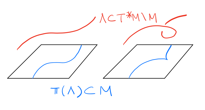
Replace the radial Liouville structure on with the Morse-Bott canonical Liouville structure on the cotangent bundle , or rather on for a Lagrangian -disk bounding a Legendrian unknot which we assume disjoint from . Then the radial Liouville cone on in gets replaced with the fibrewise Liouville cone on in , where denotes the cosphere bundle, see Figure 1.8.
Observe that as a result, the singularity gets spread out over the disk, i.e. instead of a cone on a point it is now a fibrewise cone over the disk. The skeleton of the new Weinstein structure on consists of the Lagrangian handle, union the Liouville cone on with respect to the canonical Liouville structure on , union the zero section . The singularities of this new Lagrangian skeleton are thus related to the singularities of the map , where is the front projection. These singularities correspond to the tangencies of with the distribution and are also known as caustics in the literature. For example, if has no caustics, then it is an immersion and so by axiom (v) of Definition 1.1, after a generic perturbation (to ensure self-transversality), the skeleton of is arboreal.

The idea of blowing up conical Lagrangian singularities was already present at the inception of the arborealization program, but for our purposes it is necessary to perform the blowing up procedure globally, at the level of Weinstein structures. This strategy was successfully implemented by Starkston in [St18] for the -dimensional case. Starkston moreover showed how to explicitly arborealize the semi-cubical cusp singularities which generically appear in the front projections of 1-dimensional Legendrians, thus leading to her result that 4-dimensional Weinstein manifolds always admit arboreal skeleta. In higher dimensions this strategy encounters the difficulty that there is no classification theorem for the generic singularities of front projections, nor can anything remotely close to a satisfactory classification be hoped for.
Nevertheless, there holds an h-principle for the simplification of caustics. The h-principle states that if there is no homotopy theoretic obstruction to the simplification of caustics, then the simplification can be achieved by means of a Legendrian isotopy (or for Lagrangians, by means of a Hamiltonian isotopy). Results in this direction first appeared in work of Entov [En99], and the full h-principle was established in work of the first author [AG18a], [AG18b]. Returning to our toy example, if we know that admits a polarization as in the hypothesis of our main Theorem 1.5 and we further assume that the dimension of is congruent to modulo , then it follows from the h-principle that there exists a Legendrian isotopy which deforms to a Legendrian whose front projection only has cusp singularities. In this case we can proceed as in [St18] to conclude that the skeleton of can be arborealized by a Weinstein homotopy. When the dimension of is congruent to modulo there is an additional homotopical subtlety to consider, even in this toy example, but we do not pursue this further since one also encounters additional and more serious difficulties when attempting to implement the above strategy on a Weinstein manifold with a more complicated handlebody presentation. For example, one would need to know that the relevant homotopical obstruction to applying the h-principle vanishes for every handle, yet it is unclear how to arrange for this even under the global assumption of existence of a polarization.
So instead of attempting a direct application of the h-principle, we will exploit the fact that for the purposes of arborealization we can allow deformations which are more general than a Hamiltonian isotopy, namely we can deform the skeleton of a Weinstein manifold by any homotopy of the Weinstein structure. This allows the skeleton to develop genuine singularities (i.e. non-smooth points) along which its field of tangent planes jumps discontinuously. By introducing these jumps we destroy the homotopical obstruction to simplifying the singularities with the distribution , and in fact we can always completely eliminate these tangencies.
This strategy was made precise in [AGEN19], where we introduced a class of singular Lagrangians, called ridgy, and proved an h-principle without pre-conditions, which allows one to deform any Lagrangian so that it becomes transverse to any given Lagrangian distribution, at the expense of developing ridgy singularities. This result, which we refer to as the ridgification theorem, uses the h-principle for the simplification of caustics as one of the key ingredients in its proof, but is better suited for the task at hand since there are no hypotheses needed for its application.


Ridgy singularities are extremely simple: they consist of the corner together with its products and stabilizations. Moreover, ridgy singularities can be explicitly arborealized while maintaining transversality to any given Lagrangian distribution, see Figure 1.11. So our revised strategy to arborealize a Weinstein manifold is the following: (1) blow up the singularities as before to replace Liouville cones on a point with Liouville cones on Lagrangian disks, (2) apply the ridgification theorem to get rid of all singularities of the resulting front projections, and finally (3) arborealize the ridgy Lagrangians produced by the ridgification theorem, while maintaining transversality to the relevant distributions, to obtain an arboreal skeleton for .


Finally, a word on how we deal with the issue of compatibility at the interaction of three or more strata of the skeleton: this is where the notion of positivity comes up in an essential way. The key fact is that if a Lagrangian distribution on corresponds to a family of positive definite quadratic forms, then it is transverse to the conormal of any immersed hypersurface in a neighborhood of the zero section. For the interaction of say three strata, we use the ridgification theorem to achieve transversality for two strata at a time and then conclude that transversality also holds for the third stratum for free using the above observation on positivity. This yields the desired compatibility. The existence of a global polarization for will play a key role in guiding the positivity condition globally, thus enabling the successful implementation of the above strategy.
1.5. Structure of the article
The paper is organized as follows:
In Section 2 we give the necessary preliminaries regarding Weinstein manifolds. This includes a review of notions in the literature as well as the introduction of a new framework for working with Weinstein structures. The key notions are that of a Weinstein manifold with boundary and corners, which we call a Wc-manifold, and that of a cotangent building, which provides a way of presenting a Wc-manifold in terms of successive attachments of cotangent bundles. The concept of a cotangent building gives an alternative to the standard Weinstein handlebody presentation for Weinstein manifolds, and is better suited for our purposes.
In Section 3 we prove the existence and uniqueness of symplectic neighborhoods of arboreal spaces. The existence part is an easy consequence of the stability theorem for arboreal singularities, which we proved in [AGEN20a]. The uniqueness part consists of a Darboux-Weinstein theorem for the symplectic neighborhoods of arboreal Lagrangians.
In Section 4 we discuss the notion of positivity, which is the key ingredient that allows us to control the interaction of three or more strata in the Lagrangian skeleta under consideration. We first discuss the notion of positivity for ordered tuples of Lagrangian planes, then discuss positivity for cotangent buildings and finally we relate this to the notion of positivity for arboreal spaces. We show that existence of a positive arboreal skeleton for the homotopy class of a Weinstein structure implies the existence of a polarization, proving one half of our main theorem 1.5.
In Section 5 we recall the notion of a ridgy Lagrangian from our previous work [AGEN19] and state the main result of that paper, which we call the ridgification theorem, as well as its non-integrable counterpart, which we call the formal ridgification theorem. The formal ridgification theorem also plays an important role since it holds in extension form. The main point is that by allowing for ridgy singularities we can deform any Lagrangian submanifold so that it becomes transverse to any given Lagrangian distribution, and moreover the deformation can be achieved by means of a Weinstein homotopy.
Finally, in Section 6 we show how the ridgy singularities produced by the ridgification theorem can be further deformed into arboreal singularities. Furthermore, the deformation is realized by a Weinstein homotopy and the end result is a positive arboreal Lagrangian which serves as skeleton for the deformed Weinstein structure. This proves the other half of our main theorem 1.5.
1.6. Acknowledgements
We are very grateful to Laura Starkston who collaborated with us on the initial stages of this project. We are also grateful to John Pardon who helped us to crystalize the notion of an -polarization and to Søren Galatius who explained to us how to compute obstructions to its existence.
The first author thanks the Institute for Advanced Study and Princeton University for a great research environment and thanks CRM Montreal for its hospitality. The second author thanks RIMS Kyoto and ITS ETH Zurich for their hospitality. The third author thanks MSRI for its hospitality.
Finally, we are very grateful for the support of the American Institute of Mathematics, which hosted a workshop on the arborealization program in 2018 from which this project has greatly benefited.
2. Wc-manifolds and cotangent buildings
In this section we recall the basic definitions concerning Liouville and Weinstein manifolds, and introduce the language of Wc-manifolds and cotangent buildings, which will be used throughout the text.
2.1. Liouville manifolds
2.1.1. Liouville domains
An exact symplectic manifold is a compact manifold with boundary equipped with an exact symplectic form , together with a choice of primitive , i.e. . Since is non-degenerate, the 1-form corresponds to a vector field under the contraction .
Definition 2.1.
A Liouville domain is an exact symplectic manifold such that is outwards transverse to .
Equivalently, is Liouville if is a contact form and the orientation defined on by the volume form coincides with the orientation of as the boundary of , where is itself oriented by the volume form .
We call the Liouville form and the Liouville field. By Cartan’s formula for the Lie derivative, the condition is equivalent to . This means that the vector field is symplectically conformally expanding, i.e. , , for the flow of . Equivalently, the vector field is symplectically conformally contracting and this viewpoint will sometimes be more natural in what follows. Note that we also have . The object of interest in this paper is the following.
Definition 2.2.
The skeleton of a Liouville domain is the subset
In other words, is the attractor of the positive flow of the contracting field . We will be going back and forth between Liouville domains and the closely related notion of a Liouville manifold, whose definition we recall next.
2.1.2. Liouville manifolds
Recall that the symplectization of a contact manifold equipped with a contact form for is the exact symplectic manifold equipped with the primitive , where . We can equivalently consider with for the multiplicative coordinate.
The symplectization of a contact manifold can be defined invariantly without choosing a contact form. Assuming that is connected and is co-oriented, we define as follows. Let be the total space of the conormal line bundle to and the component of consisting of -forms defining the given co-orientation of . Then is a primitive of the exact symplectic form and we define as endowed with this structure. A choice of a contact form for identifies with and with . For example, the symplectization of the cosphere bundle is the complement of the zero section in .
In the other direction, the contactization of an exact symplectic manifold is the manifold equipped with the contact form , where . For example, the contactization of the cotangent bundle is the 1-jet bundle .
Definition 2.3.
A finite type Liouville manifold consists of a (non-compact) boundaryless exact symplectic manifold such that the following conditions hold.
- (L1)
The vector field which is -dual to is complete for .
- (L2)
There exists a compact domain such that is outward transverse to the boundary , i.e. is a Liouville domain, and such that the union of forward trajectories of starting at is equal to .
We call Liouville domains as in (L2) defining.
Definition 2.4.
The skeleton of a finite type Liouville manifold is defined to be
Clearly, for any defining Liouville domain . Hence the skeleton of a finite type Liouville manifold is compact. Note that for any such we may use the Liouville flow starting at to parametrize as . Since the Liouville field conformally expands we have for the coordinate parametrizing the Liouville flow, so is the positive part of the symplectization of the contact manifold .
Conversely, any Liouville domain can be completed to a Liouville manifold by attaching to it the positive part of the symplectization of . Explicitly:
where the Liouville form on extends to to as .
Definition 2.5.
The ideal boundary of a finite type Liouville manifold is defined to be , where the action is given by the positive flow of .
Since , the form descends to as a contact structure . A choice of a contact form for yields an isomorphism which maps contactomorphically onto the boundary of a defining Liouville domain. We denote by the projection along the trajectories of .
2.1.3. Deformations of Liouville structures
Definition 2.6.
A homotopy of finite type Liouville structures is a family , , of finite type Liouville structures on a manifold admitting a smooth family of defining Liouville domains.
Given such a homotopy there exists an isotopy such that , where . Moreover, one can always arrange that for uniformly compactly supported functions , see [CE12], Sections 11.1 and 11.2. In particular, it is always sufficient to consider homotopies fixing the symplectic form, and moreover changing the Liouville form by adding a compactly supported exact form. Note that for any fixed the space of Liouville structures on which are fixed at infinity is convex, hence any two such Liouville structures are canonically homotopic.
Remark 2.7.
Unless explicitly stated otherwise, all Liouville structures under consideration in this paper are of finite type and hence we will stop mentioning this below.
We will often abuse terminology and say that two Liouville manifolds and are Liouville homotopic if there exists a symplectomorphism such that is a Liouville manifold which is Liouville homotopic to . In all cases where such terminology will be abused, the symplectomorphism will be obvious and unique up to contractible choice.
If on the nose, we say that and are Liouville isomorphic. For and Liouville domains or manifolds we call a smooth, proper embedding a Liouville embedding if .
2.1.4. Liouville germs
It will often be convenient to express our constructions in the language of germs.
Definition 2.8.
A Liouville germ is the equivalence class of defining Liouville domains for a fixed Liouville manifold .
Definition 2.9.
A Liouville embedding of a Liouville germ into a Liouville domain or manifold is an equivalence class of Liouville embeddings , where is a defining domain for and we identify with if they agree on a defining domain for contained in both and .
Example 2.10.
The cotangent bundle of a closed manfiold is a Liouville manifold with the canonical 1-form. The Liouville field is the fibrewise radial vector field and the skeleton is the zero section . As a Liouville domain we can take the unit disk bundle relative to any Riemannian metric on . The ideal boundary is the cosphere bundle , i.e the (positively) projectivized cotangent bundle, which is contactomorphic to the unit sphere bundle for any choice of Riemannian metric. We will use the notation for the germ of the cotangent bundle .
2.2. Weinstein manifolds
2.2.1. Lyapunov functions
Let be a Liouville manifold. While always has its -dimensional Lebesgue measure equal to , its dimension can nonetheless be quite large if no extra conditions are imposed on the Liouville structure. For example, McDuff constructed in [MD91] a Liouville structure on for a closed surface of genus whose skeleton has codimension 1. To tame the dynamics of the Liouville flow we require existence of a Lyapunov function.
Definition 2.11.
We say that is a Lyapunov function for the Liouville manifold if is gradient-like for , i.e. if there holds
- (W1)
for some Riemannian metric on and some constant .
Note that the space of Lyapunov functions for a given Liouville structure is convex, hence contractible as soon as it is nonempty. Consider the set of critical points of the Lyapunov function, which by (W1) is the same as the zero set of the Liouville form. The conditions (L1) and (W1) imply that is the union of the -stable manifolds of the critical points of , i.e. points converging to in forward time. However, as far as we know, we have to add some further constraints on the Lyapunov function in order to deduce any meaningful properties.
Definition 2.12.
A Morse-Weinstein manifold is a Liouville manifold for which there exists a Morse Lyapunov function .
Under this assumption it was shown in [CE12], see also [EG91, E95], that
- (W2)
is the union of submanifolds which are isotropic for , and hence for .

Remark 2.13.
Note that -isotropic is equivalent to -isotropic and -conic.
Without any assumptions on , is not known whether a triple which satisfies (L1), (L2) and (W1) is homotopic in the class of such triples to one with a Morse Lyapunov function. However, condition (W2) holds for a larger class of taming functions, for example when is generalized Morse, see [CE12]. Moreover, it is often most natural to consider a Lyapunov function which is not Morse or even generalized Morse, such as the Morse-Bott function on .
2.2.2. Morse-Bott Lyapunov functions
In this paper we will consider a version of Morse-Bott Weinstein structures which allows the critical set of the Lyapnuov function to have nonempty boundary, and even corners. Our definition is a slight variation of Starkston’s definition in [St18] of a Weinstein structure which is Morse-Bott with boundary.
Let be the decomposition of the tangent space to at a zero of into generalized eigenspaces of the differential with eigenvalue having positive, zero or negative real part respectively. Suppose first that a connected component of is a smooth, proper submanifold of without boundary. Then the Morse-Bott condition on a triple along the component is the following:
- (MB1)
is non-degenerate in the directions normal to , i.e. .
When we moreover demand that in a neighborhood of the triple takes a special form, which we now describe. Recall the Weinstein normal form for Morse critical points in a Weinstein manifold of dimension . There are two possibilities depending on the index: or .
- ()
, .
- )
, .
We also recall the standard Morse-Bott normal form corresponding to the canonical Liouville structure on .
- (std)
, .
We construct local models for Morse-Bott with boundary Weinstein structures on with the half line as the critical set. The construction consists of patching up the above Morse normal forms on the half plane with the standard Morse-Bott normal form on the half plane . Take any smooth function satisfying the following properties:
- (i)
on
- (ii)
on for some .
- (iii)
and on for that same .
In the case we set and in the case we set . In both cases the patched up model is then given by , which has Liouville field for the Hamiltonian vector field of . Explicitly, when we have
Since the coefficient which multiplies is positive, we deduce that admits a Lyapunov function. For example, if we set for
then is the Euclidean gradient of along and we have on all of , from which the claim follows. Similarly, one verifies that also admits a Lyapunov function.
Definition 2.14.
We call the Weinstein normal form for Morse-Bott boundary of index .

The space of permissible is convex, hence the normal form is well defined up to a contractible choice. Note that the behavior of the Liouville flow along the half line , which shares its boundary point with the critical set , can be either repelling or attracting depending on whether or . We also consider products of these normal forms. Thus we obtain Weinstein structures on where the critical set is the positive quadrant , which not only has boundary but also has corners of all orders .
Definition 2.15.
The Weinstein normal form for Morse-Bott -fold corners of index is the product of copies of and copies of .
Going back to a triple as before, consider a component of the critical set of such that is a smooth, proper submanifold of with nonempty boundary and possibly with higher order corners. By definition, if is a corner of order , then there is a collar neighborhood of in , where is the germ of the interval at and is a neighborhood of in the order corner locus. For such a collar neighborhood we have a local symplectomorphism near between and , with corresponding to . The condition we require is that for each such -fold point there exists a collar neighborhood as above such that with respect to the splitting there holds:
- (MB2)
splits as a direct sum with the summand corresponding to given by the canonical Liouville form and the summand corresponding to given by the Weinstein normal form for Morse-Bott -fold corners for some .
Definition 2.16.
A generalized Morse-Bott Weinstein manifold is a Liouville manifold which admits a Lyapnuov function whose critical set is a union of smooth, proper submanifolds with corners satisfying (MB1) and (MB2).
Remark 2.17.
It was shown by Starkston [St18] that in the boundary repelling Morse-Bott case the intersection of the -stable manifold of a component of the critical set of with a neighborhood of is a smoothly embedded isotropic submanifold of , even without requiring standard local models. To check that this property also holds near the boundary attracting or mixed behavior points of the Morse-Bott structures considered above is straightforward, since it suffices to consider the explicit local model.
Lemma 2.18.
Suppose that is a generalized Morse-Bott Weinstein manifold. Then there exists a homotopy , fixed outside of a compact subset, such that is Morse-Weinstein for .
Proof.
We give the proof in the case where each component of the critical set of is of the critical dimension , the general case is similar and in any case will not be needed for our purposes. Suppose first that has empty boundary. Since is Lagrangian, by the Weinstein neighborhood theorem it has a neighborhood in symplectomorphic to a neighborhood of the zero section in . Therefore we may from the onset replace by with the pulled back Liouville form which we still denote by .
Let be a Morse function and let be a cutoff function such that on and outside of a slightly bigger neighborhood. Fix an auxiliary Riemannian metric on and put , a function on . The restriction of the Hamiltonian vector field of the function to is . Hence is a Lyapunov function for in a neighborhood of and therefore on all of if is taken sufficiently small. Moreover, for such the Liouville form is Morse-Weinstein for any .
If is non-empty, then we need to modify the construction somewhat. Consider a slight enlargement of in obtained by attaching an isotropic collar along so that the Liouville field is tangent to . Then we should require that our function is Morse on , compactly supported in , has no critical points on and moreover has the following behavior on . Let be the closure of a component of the order 1 corner locus . If the Liouville structure is boundary attracting along , then we demand that for any inwards pointing vector . If the Liouville structure is boundary repelling () along , then we demand that for any outwards pointing vector . With this restriction on the proof proceeds just as before. ∎
Remark 2.19.
As we will see, if a Morse-Bott Weinstein manifold has arboreal skeleton, then one can choose the Morsifying homotopy such that for all .
2.2.3. Weinstein manifolds
It is easy to check that Lemma 2.18 also holds for the generalized Morse condition instead of Morse-Bott, see Proposition 9.13 in [CE12]. Therefore we will take the following as our working definition, which includes Morse, generalized Morse and Morse-Bott Weinstein structures.
Definition 2.20.
A Liouville manifold is called Weinstein if there exists a Liouville homotopy and a family of Lyapunov functions for such that is Morse-Weinstein for .
The notions of a Weinstein domain, defining Weinstein domain for a Weinstein manifold and a Weinstein germ are entirely analogous to the corresponding notions in the Liouville case. We emphasize that the Lyapunov function is not part of the structure of a Weinstein manifold, we merely require its existence. For example, Weinstein embeddings are just Liouville embeddings of Weinstein type Liouville manifolds (or domains, or germs). We do not require the embedding to pull back one Lyapunov function to the other. Similarly, a Weinstein isomorphism (resp. homotopy) is a Liouville isomorphism (resp. homotopy) of Liouville manifolds of Weinstein type.
Example 2.21.
The standard Liouville structure on the cotangent bundle of a closed manifold is Weinstein. Given a Riemannian metric on , the function is a Morse-Bott Lyapunov function for . By the procedure explained in Lemma 2.18, we can Morsify the Lyapunov function using a Morse function on . By inspection, this procedure does not change the skeleton of , which is the zero section.
Remark 2.22.
Although Definition 2.20 allows for rather degenerate Weinstein structures, in the Weinstein homotopies constructed in this paper for the purposes of arborealization of a Morse-Weinstein manifold the Weinstein structures are always of Morse-Bott type except for a finite number of times at which there is a birth/death of Morse-Bott critical components.
2.3. Wc-manifolds
2.3.1. Manifolds with boundary and corners
Recall that an -dimensional smooth manifold has a corner of order at if there is a neighborhood of in diffeomorphic to a neighborhood of the origin in , where denotes the germ of the interval at . We denote the locus of order corners by . The closure of a connected component of is called a boundary -face. For we will more simply call a boundary face. Sometimes we will call a manifold with boundary and corners (of any order) a bc-manifold for short.
We always assume that each component of is regularly embedded, so that each -face is itself a manifold with corners. Under this assumption, if is a -face, then there is an embedded collar neighborhood . We consider the germs of these collars as part of the structure. In particular, near each point we have canonical collar coordinates , where and . Note that in a neighborhood of we have cut out by . More generally, for the components of whose closure contains are given by setting exactly of the coordinates equal to zero.
We demand compatibility of these collars in the sense that the remaining coordinates give the collar structure for near . We call such a compatible system of collar germs a corner structure on . Henceforth all manifolds with corners will be implicitly equipped with a fixed but otherwise arbitrary corner structure.

Let us choose a partial ordering of the boundary faces of a manifold with corners such that the faces at all corners are ordered in a compatible way, i.e. the order is that induced by the order of the coordinates in the collar structure. We will assume this order to be part of the structure of a manifold with corners.
Given manifolds with corners and , we consider embeddings of into which satisfy the property that each -face of is properly embedded into some -face of , where .
2.3.2. Liouville manifolds with boundary and corners
We now give an inductive definition of the notion of a Liouville manifold with corners of order , starting with the base case which is just our previous definition.
Definition 2.23.
A Liouville manifold with corners of order consists of an exact symplectic manifold with smooth corners of order such that the following properties hold.

- (L1)
The vector field which is -dual to is complete for .
- (L2)
There exists a compact domain with corners such that such that is outwards transverse to its vertical boundary , which is defined to be the closure of , and such that the union of forward trajectories of starting at is equal to .
- (L3)
For , each -face of the horizontal boundary , which is defined to be , contains a Liouville submanifold with corners , called the nucleus of , such that the collar neighborhood of in is of the form , where is the product of with the cotangent fibre over , and in this neighborhood the form is the direct sum of a Liouville form on and the canonical 1-form on .
It follows from the definition that the Liouville field is tangent to every component of , . A Liouville manifold with corners has a horizontal boundary and an ideal vertical boundary , where just as before the action of is defined by the flow of and the skeleton is defined to be the attractor of the negative flow of .
We call as in (L2) a defining Liouville domain with corners for the Liouville manifold with corners . Note that the horizontal boundary of is and its vertical boundary , the closure of , is a contact manifold with corners which is naturally contactomorphic to under the projection . Just as before, the equivalence class of defining domains for Liouville manifold with corners is called the Liouville germ of and is denoted by . Notions of isomorphism and homotopy of Liouville manifolds with corners are defined exactly the same way as without corners.
2.3.3. Wc-manifolds
We now introduce Weinstein structures for Liouville manifolds with corners, which we call Wc-manifolds. We restrict our discussion to the Morse-Bott category since this is the framework in which we will work throughout this paper.
Definition 2.24.
A Wc-manifold is a Liouville manifold with corners whose Liouville vector field admits a Morse-Bott Lyapunov function , i.e. satisfying (MB1) and (MB2) in the interior of , and such that on the collars of (L3) has the form for a Morse-Bott Lyapunov function on and the momentum coordinates on .

Defining Liouville domains for Wc-manifolds will be called defining Wc-domains, and the equivalence class of such will be called a Wc-germ. Notions of Wc-isomorphism, embedding and homotopy are the same as the corresponding notions for Liouville manifolds with corners, but demanding that all objects in sight are of Weinstein type.
Example 2.25.
Let be a smooth -dimensional manifold with corners. Then is a Liouville manifold with corners, where the structure (L3) is induced by a corner structure on . We call the germ of a cotangent block. The corresponding Lagrangian distribution tangent to cotangent fibers will be denoted by . We denote by and the corresponding Liouville form and the Liouville vector field. The notation will be used for the positively projectivized cotangent bundle of , which is the ideal boundary of . For a -face of we have a -face of and is the nucleus of . The collar coordinates near yield the decomposition . A choice of Riemannian metric on yields defining Liouville domain with corners and a Morse-Bott Lyapunov function .
The rest of this section can be equally discussed in the Liouville and Weinstein categories. We restrict the discussion only to the Weinstein case as this is the one needed for our further applications.
2.4. Wc-hypersurfaces
2.4.1. Weinstein hypersurfaces
We now turn our attention to Weinstein hypersurfaces with corners, or Wc-hypersurfaces. They were introduced (without corners) in [E18]. These are special cases of the Liouville hypersurfaces introduced by Avdek in [A12]. This notion is similar to the “stops” of Sylvan, [Sy16] and the Liouville sectors of Ganatra-Pardon-Shende, [GPS17]. Related constructions are also considered in Ekholm-Lekili’s paper [EL17]. We first recall the definition without corners.
Definition 2.26.
A Weinstein hypersurface in a Weinstein manifold is a Weinstein embedding such that is an embedding.
Note that any Weinstein hypersurface is contained in a boundary of some defining domain . Note also that the Reeb vector field of the contact form is transverse to . Note also that the boundary is a codimension 2 contact submanifold of . By the assumption that is Weinstein, the skeleton can be decomposed as a union of isotropic submanifolds, which in the top dimension are Legendrian for the contact structure .
Lemma 2.27.
The skeleton depends only on the projection .
Proof.
Indeed, the Liouville fields corresponding to the Liouville structures and for a positive function are proportional. In fact, as computed in Lemma 12.1 of [CE12] the form is symplectic if and only if , where is the expanding field for , and in that case the restriction of the form to is automatically Liouville, with the expanding vector field for equal to . Therefore only depends on the contact structure . ∎
Note that the space of functions for which is Liouville (and hence in the considered case Weinstein) is convex, therefore contractible.
Definition 2.28.
We say that two Weinstein hypersurfaces in a Weinstein manifold are related by a translation if for some function .
Note that given a defining domain , any Weinstein hypersurface of can be translated to a Weinstein hypersurface contained in . However, it may not be possible to translate it to a Weinstein hypersurface contained in . Indeed, this is equivalent to the condition for the conformal factor between the contact forms corresponding to and .
Definition 2.29.
A Weinstein hypersurface germ is an equivalence class of Weinstein hypersurfaces for defining domains for a fixed Liouville manifold, where two embeddings are equivalent if they agree on a smaller defining domain, possibly after translation.
One can think of as living in the ideal boundary , or one can think of as the germ of a Weinstein embedding . The two viewpoints are equivalent and we will go back and forth between them.
Example 2.30.
An important example of a Weinstein hypersurface is the ribbon of a Legendrian submanifold. Let be a Legendrian submanifold in the contact boundary of a Liouville domain . Then it admits a Darboux neighborhood contactomorphic to for some Riemannian metric on . The strip is a Weinstein hypersurface symplectomorphic to the cotangent disk bundle of , whose skeleton is precisely . The space of all ribbon extensions of a given Legendrian is contractible. An important example to keep in mind is the case where for a smooth manifold, with respect to any Riemannian metric on and is the unit conormal to a co-oriented hypersurface .

2.4.2. Weinstein pairs
Definition 2.31.
A Weinstein pair consists of a Weinstein manifold together a Weinstein hypersurface .
We will also call a Weinstein pair when is the germ of a Weinstein hypersurface .
Definition 2.32.
Let be a Liouville manifold and any subset. The Liouville cone on is the saturation of by the Liouville trajectories:
The positive Liouville cone on is the saturation of by the backwards Liouville trajectories:
Note that if is compact, then has compact closure while does not. The skeleton of a Weinstein pair is defined as the compact subset:
Note that for any defining domain such that , moreover . The notion of a pair at the level of germs is defined as follows.
Definition 2.33.
A Weinstein (germ) pair consists of a Weinstein germ together with a Weinstein hypersurface germ .
Note that for any representative of we may take a representative for contained in . The skeleton of a Weinstein pair is defined as the non-compact subset:
Equivalently in terms of germs, we can think of as the equivalence class of the compact subsets for all defining domains and representatives for such that .
2.4.3. Wc-hypersurfaces
Finally, we extend the above to include boundary and corners.
Definition 2.34.
A Wc-hypersurface in a Wc-manifold is an equivalence class of embeddings of Wc-germs such that is an embedding, with the equivalence given by translation.
All the previous discussion carried over word by word to the Wc-setting. The notion of a Weinstein pair in the Wc-category is called a Wc-pair.
Definition 2.35.
A Wc-pair consists of a Wc-germ together with a Wc-hypersurface germ .
2.5. Conversion between Wc-hypersurfaces and face nuclei
2.5.1. Nucleus-to-hypersurface conversion
We start with a Wc-manifold . Let be a boundary face of and its nucleus. Let be a collar neighborhood of in as in the definition of a Wc-manifold. So is of the form , with where is the defining coordinate for . Attach to the half-infinite collar along their common intersection and on the union consider the Weinstein structure given by the direct sum of and the Weinstein normal form for Morse-Bott boundary of index , which agrees with on . The existence of a Morse-Bott Lyapnuov function is immediate from the local model. Hence the result is a Wc-manifold . Let be the germ of . For note that is a Wc-hypersurface for . Any two differ by a translation and all are canonically identified with . We will denote this Wc-hypersurface by .
Note that by construction we have . The operation only depends on the contractible choice of a collar neighborhood and the contractible choice of the Weinstein normal form for Morse-Bott boundary. Hence it produces a Wc-germ which is well defined up to Wc-homotopy.
Definition 2.36.
The Wc-pair is called the nucleus-to-hypersurface conversion of the Wc-germ and the boundary nucleus .
2.5.2. Underlying Weinstein manifold of a Wc-manifold
Let be a Wc-manifold and let be a boundary face. The resulting of converting the nucleus of to a Wc-hypersurface is a Wc-manifold which has one less boundary face than . We can continue this process inductively over all faces. After forgetting the resulting Wc-hypersurfaces, we end up with a Weinstein manifold without boundary which we denote . It is clear that the Weinstein homotopy class of the Weinstein manifold does not depend on the order in which the boundary faces are chosen. If one wishes to, one can further deform the Weinstein structure on , which at this point is generalized Morse-Bott, so that it becomes Morse-Weinstein.
Definition 2.37.
The Weinstein manifold obtained from a Wc-manifold by converting all of its boundary nuclei to Wc-hypersurfaces is called the underlying Weinstein manifold.
Example 2.38.
the underlying Weinstein manifold of the Wc-manifold is Weinstein homotopic to .
Remark 2.39.
A Wc-manifold may be thought of as a Weinstein manifold with ‘stops’. From this viewpoint, taking the underlying Weinstein manifold of a Wc-manifold is simply removing the stops.
2.5.3. Hypersurface-to-nucleus conversion
The converse operation to the nucleus-to-hypersurface conversion is the hypersurface-to-nucleus conversion, which we discuss next. Here and below we denote .
Lemma 2.40.
The inclusion of a Wc-hypersurface extends, uniquely up to contractible choice, to a Liouville embedding , where is identified with .
Proof.
Let be a defining domain such that and let be its contact surrounding, as in [E18], so that the restriction of to this neighborhood is of the form , where is the projection and . For every , let denote the backwards flow of starting at , where . For every , let denote the backwards flow of starting at , where . We extend the contact embedding which sends to a Liouville embedding by sending , so that by construction is identified with . It is clear that the embedding is determined by the contact surrounding and its parametrization, which are unique up to contractible choice. ∎
We now explain the hypersurface-to-nucleus conversion. Let be a Wc-manifold and let be a Wc-hypersurface. Fix defining Wc-domains and for and respectively so that we have an embedding which extends to an embedding as in Lemma 2.40. Consider the exact symplectic manifold which is the result of gluing and along . Consider the Weinstein structure on , thought of as the -neighborhood of the zero section in , which is the restriction of the Weinstein normal form for Morse-Bott boundary of index translated two units in the direction, so that the critical set is . The restriction of this structure to is , hence we obtain a patched up structure on the union of and . Moreover, by inspection the new Liouville field points outwards at the boundary. So we may replace with a smoothing for a function satifying
- (i)
as
- (ii)
on
- (iii)
on
and the Liouville field is still outwards pointing for the smoothed boundary. Thus we obtain a defining domain for a Wc-manifold . Indeed the only think that needs to be checked is the existence of a Morse-Bott Lyapunov function, which is clear from the local models since without loss of generality we can start with a defining domain for such that is a regular level set of the Morse-Bott Lypanuov function for . Note that is the nucleus of the new boundary face of .
By construction we have , or more precisely
In other words, the backwards -Liouville cone on has a trivial collar attached to it, which does not change the topology of . Note that the space of possible smoothings is convex, hence contractible. The choice of Morse-Bott Weinstein normal form is also contractible. Similarly the choice of collars used in the construction is contractible. Hence we get a Wc-germ which is well defined up to Wc-homotopy. Finally, note that different representatives for will also result in homotopic Wc-manifolds . Hence the conversion operation only depends on the Wc-hypersurface germ up to Wc-homotopy.
Definition 2.41.
The Wc-germ is called the hypersurface-to-nucleus conversion of the Wc-germ and the Wc-hypersurface .
2.5.4. Cancellation of conversions
The hypersurface-to-nucleus conversion is inverse to the nucleus-to-hypersurface conversion at the level of Weinstein homotopy classes, as follows from a parametric Smale cancellation of Morse-Bott index and critical points, the existence of which is immediate from the local models. This implies the following obvious but important lemma.
Lemma 2.42.
Let be the result of hypersurface-to-nucleus conversion of a Wc-hypersurface . Then the underlying Weinstein manifolds of and are Wc-homotopic.
2.6. Gluing and splitting
2.6.1. Horizontal gluing
We will now describe the basic gluing operation for Wc-manifolds. Given two Wc-manifolds and , we define their horizontal gluing as follows. Pick some non-adjacent boundary faces of and of , and for each suppose we are given a Liouville isomorphism , where and are the nuclei or and respectively. We have collar neighborhoods and and we extend to as .
Definition 2.43.
The horizontal gluing of and along is defined to be the Wc-germ of the Wc-manifold where we identify via .
Example 2.44.
Suppose are two manifolds with boundary and we have a diffeomorphism . Then lifts to a Liouville isomorphism between and and we can perform the horizontal gluing which is the same as for the smooth gluing of and given by .

Note that the skeleton of the horizontal gluing of and is equal to the union of the skeleta of and .
2.6.2. Vertical gluing
We can also glue two Wc-manifolds and in a different way.
Definition 2.45.
Suppose we have a Wc-hypersurface in and a Liouville isomorphism for the germ of the nucleus of a boundary face of . The vertical gluing of and is defined to be the composition of two steps: a conversion a Wc-hypersurface into a boundary hypersurface, see Section 2.5 above, followed by a horizontal gluing.

Indeed, if we first convert into a boundary nucleus, we can then apply the horizontal gluing determined by as descibed above. The resulting Wc-germ is well defined up to Wc-isomorphism. Note that the skeleton of the vertical gluing is equal to the union of the skeleton of the pair and the skeleton of . We record for future reference the following slight strengthening of this observation, where we denote by the Liouville form for the defining coordinate of a boundary face .
Lemma 2.46.
Let , be two Wc-germs, a Wc-hypersurface, the nucleus of a boundary face of and its germ, a Liouville isomorphism and the result of vertically gluing to along . Then there exists a symplectic embedding of germs such that the following properties hold, where we denote by the restriction of the inclusion to the interior of .
- (i)
- (ii)
.
- (iii)
and .
Proof.
We recall from the gluing construction that we attached to the top of a cylinder . Since a neighborhood of in is symplectomorphic to , we can map symplectomorphically to , relative to say, so that the symplectomorphism extends to the rest of as the identity. Moreover, the symplectomorphism can be obtained from a reparametrization of the coordinate, hence the Liouville forms pull back as desired. ∎
2.6.3. Splitting
The converse operation to gluing is splitting.
Definition 2.47.
Given a Wc-manifold , a regularly embedded hypersurface with corners called splitting for if it satisfies the following conditions:
- (i)
divides into two parts, and , which are manifolds with corners.
- (ii)
the Liouville vector field of is tangent to .
- (iii)
there exists a hypersurface with corners tangent to .
- (iv)
is a Wc-manifold and there exists a retraction such that .
Remark 2.48.
That is regularly embedded implies in particular that .
We will refer to as the soul of the splitting hypersurface and denote it by . Note that .
Example 2.49.
Let be a manifold with corners and a regularly embedded codimension submanifold with corners, so that . Assume that divides into two parts: and , so that . Then is a splitting hypersurface. Given a decomposition of the tubular neighborhood of , , we have the soul of .
The splitting hypersurface can be used to split into two Wc-manifolds in two ways, horizontal and vertical. For the horizontal splitting we view as Wc-manifolds with an additional component of . The Wc-manifold serves as the nucleus of the additional boundary component . The vertical splitting consists of a horizontal splitting followed by a nucleus-to-hypersurface conversion operation, transforming the nucleus into a Wc-hypersurface.
2.6.4. Partial horizontal gluing
One more basic operation that we will need is the creation of corners and its associated partial horizontal gluing. Let be a Wc-manifold, a boundary face of and the nucleus of . Let be a splitting hypersurface with soul . Then there is a deformation of the Wc-structure on which creates an additional corner along with its nucleus .
More precisely, take a collar neighborhood , so that and extend it to with the same Liouville form. Let be a tubular neighborhood of in and consider a smooth function satisfying the following properties:
- (i)
as .
- (ii)
on
- (iii)
on .
Set and consider the subset consisting of points such that . Then the union of and along is a new Wc-manifold which has a new corner along a parallel copy of .

Next, consider two Wc-manifolds with boundary faces and respective nuclei . Let be a dividing hypersurface for with its soul , which splits into Wc-manifolds and , which share a common face with the nucleus . Suppose there is a Liouville isomorphism .
Definition 2.50.
The partial horizontal gluing of to using is the Wc-germ obtained from the following two operations:
- (a)
Creating a corner along , i.e. adding to , and replacing the face with two faces ;
- (b)
The horizontal gluing and along .
As before, the partial horizontal gluing is well defined up to Wc-homotopy.
2.7. Wc-buildings
2.7.1. Iterated gluing
We now introduce the iterated vertical gluing of Wc-manifolds, which will be a convenient notion for the constructions in this paper. Consider Wc-germs . We inductively define a -level Wc-building, which we will denote by , as the following presentation of a Wc-germ.
Definition 2.51.
A -level Wc-building is itself. Suppose that the Wc-building
is already defined. Consider a nucleus of one of the boundary faces of and let be an embedding as a Wc-hypersurface in . The building
is by definition the result of a vertical gluing of and along .

So a Wc-building is a Wc-germ equipped with a choice of presentation of its Wc-deformation class as the iterated vertical gluing .
2.7.2. Distinguished cover of a Wc-building
A Wc-building come equipped with a symplectic cover by the Wc-manifolds it is built out of. The relevant properties of this cover are summarized in the following lemma. Recall that given a Wc-manifold the Liouville form restricted to a neighborhood of a face has the form where is the nucleus of and is the defining coordinate for the face . We recall the notation for the form on .
Lemma 2.52.
Suppose is presented as a -level building . Then there exist symplectic embeddings , , such that
- (i)
;
- (ii)
if ;
- (iii)
If for then there exists a nucleus of a boundary face of such that and

Proof.
We inductively construct the maps , , as follows, at the end of the inductive process we will set . The map is just the inclusion on into . Suppose we have defined maps for . Recall that is vertically glued to by a Liouville isomorphism between the nucelus of a boundary face of and a Wc-hypersurface in . Let be the symplectic embedding from Lemma 2.46, set and set to be the restriction of the inclusion to the interior of . The desired properties for the resulting follow from the properties stated in Lemma 2.46. ∎
Remark 2.53.
Note that on the overlap the pushed-forward Liouville fields coming from all commute with each other.
2.7.3. Cotangent buildings
Finally, we introduce a particular class of Wc-buildings which will be particularly relevant for our purposes.
Definition 2.54.
A Wc-building for which each Wc-germ consists of a cotangent block is called a cotangent building.
We will later show that any finite type Weinstein manifold can be realized as the underlying Weinstein manifold of a cotangent building.
2.8. Legendrian submanifolds
2.8.1. Legendrians in cotangent bundles
Consider first a cotangent bundle , where an -dimensional compact manifold with corners. Let be an -dimensional manifold with corners.
Definition 2.55.
An embedding is called Legendrian if its projection to is a Legendrian embedding.
With every Legendrian we associate its Lagrangian Liouville cone formed by forward and backwards trajectories of the Liouville field . Note that is embedded.
The splitting near a -face of provide canonical splittings
| (1) |
We will call a Legendrian embedding adapted to the block if and for each stratum we have for a Legendrian .
By conical Lagrangians we will always mean Lagrangian Liouville cones over Legendrians.
Denote by the cotangent bundle projection.
Definition 2.56.
An adapted Legendrian is called regular if is an immersion with transverse self-intersections.
2.8.2. Legendrians in Wc-manifolds
Let be a -dimensional Wc-manifold.
Definition 2.57.
An -dimensional submanifold is called Legendrian if it projects to as an embedded Legendrian submanifold of . Its Liouville cone is a called a conical Lagrangian.
We say that a Legendrian is adapted to the Wc-structure of if and moreover in a neighborhood of any corner we have , where is a Legendrian in the nucleus of the corner .

Example 2.58.
Let be a manifold and a co-oriented hypersurface. Then any submanifold which 1-1 projects to the conormal lift of in (and is never tangent to the Liouville flow) is Legendrian. If is adapted for the corner structure of , then one can construct a Legendrian lift which is adapted for the Wc-structure of .
We can also think of Legendrians in as equivalence classes of Legendrian embeddings into defining domains for , where the equivalence is given by translation along the Liouville flow. This gives us the notion of a Legendrian in a cotangent block . Similarly, we have the notion of a Legendrian in a Wc-germ . For a Legendrian in a defining domain for , we only take its positive Liouville cone , which is contained in . One can think of the equivalence class of all positive Liouville cones over all Legendrians equivalent to as the whole Liouville cone .
2.9. Gluing and splitting of Legendrians
2.9.1. Gluing Legendrians
Lemma 2.59.
Let be a Wc-germ, an adapted Legendrian and the -Liouville cone over . Let be the result of a nucleus-to-hypersurface conversion of the nucleus of one of the boundary faces of . Then remains Legendrian and its -Liouville cone coincides with .
Proof.
In a neighborhood of the face of whose nucleus we convert to a boundary face we have and . The conversion changes only by the differential of a function of , moreover the resulting Liouville field on is tangent to (and outwards pointing at the boundary). Hence remains Legendrian and its Liouville cone is unchanged. ∎
Lemma 2.60.
Let be two Wc-germs, two of their boundary faces and the nuclei of . Let and be two adapted Legendrians. Denote , . Let be a Liouville isomorphism such that . Then the horizontally glued Wc-manifold contains a glued Legendrian
Proof.
This is obvious by definition of adapted. ∎
2.9.2. Splitting Legendrians
Let be a Wc-manifold and a splitting hypersurface with the soul . A Legendrian is called in in splitting position if is transverse to and .
Lemma 2.61.
Let be a Wc-manifold, a splitting hypersurface and consider a Legendrian which is in splitting position. Then under a horizontal splitting of we can arrange it so that splits into Legendrians with corners .
Proof.
It suffices to take a neighborhood of in so that is of product form with respect to the neighborhood, which is clearly possible. ∎
Let us recall that given a contact manifold a hypersurface is called convex if it admits a tranverse to it contact vector field . Consider a split a tubular neighborhood of a contact hypersurface such that the contact vector field coincides with , where is the coordinate corresponding to the second factor. The contact structure on can be then defined by a contact form , where is a smooth function and is a 1-form on . The set is called the dividing set. It is always a regular level set of the function . Denote . We also denote
and call it the dividing wall. The contact condition implies that is a contact form on and that the form is Liouville on . The corresponding Liouville fields are complete of both halves and and for any point there exists a limit . We say that the pair , where is a convex hypersurface and a transverse vector field, is of Weinstein type, if is Weinstein.
Lemma 2.62.
Let be a contact manifold, a Weinstein type convex hypersurface and a Legendrian transverse to . Then there exists a contact isotopy , such that
- (i)
fixes ;
- (ii)
leaves invariant;
- (iii)
there exists such that ;
- (iv)
is supported in a neighborhood .
Proof.
Note that a contact vector field on smoothly extends to as equal to on . Let us choose sufficiently small so that the coordinate has no critical points. Denote . A general position argument allows us to -perturb so that and the projection of along Liouville trajectories of is an embedding. Note that , and hence is Legendrian for the contact structure on . Let us parameterize by an embedding such that . Define a Legendrian isotopy , by the formula
Let us observe that , with flowing a -isotropic submanifold to along trajectories of . The flow is fixed on . Let us analyze the isotopy in a neighborhood of . The form on can be written as for the coordinate on , and hence, . The flow is given by . Assuming that is large enough so that we get as . Hence by reparameterizing the isotopy to the interval and extending it to the end-point as . we get a smooth Legendrian isotopy such that . The isotopy can be realized by an ambient contact isotopy which keeps invariant. By cutting off this isotopy outside a smaller neighborhood of we get the required Legendrian isotopy of . ∎
Lemma 2.63.
Consider a Wc-manifold with a dividing hypersurface and its soul . Let be any Legendrian. Then there exists a Legendrian isotopy , , such that is in a splitting position.
Proof.
We can realize as a smooth boundary of a neighborhood of and view and as submanifolds of . Then the boundary is a convex hypersurface in the contact manifold , and its dividing set divides into two copies of . Therefore the conclusion follows from the previous lemma. ∎
2.9.3. Legendrians in Wc-buildings
Let be a Wc-germ with a structure of a -block building . We say that a Legendrian is compatible with the building structure if its Liouville cone is invariant with respect to all Liouville fields , , which we can think of as living in via Lemma 2.52.
Lemma 2.64.
Let be presented as a Weinstein building . Let be a Legendrian. Then there exists a Legendrian isotopy starting from such that is compatible with the building, i.e. its -Liouville cone is invariant with respect to all Liouville fields where they are defined.
Proof.
By definition we have filtration by Wc-manifolds , where . Note that we equivalently view as a 2-block building . By definition the building can be split into the blocks and along a splitting hypersurface which can be defined as follows. Recall that is obtained from and by taking the nucleus of one of the boundary faces of , realizing it as Wc-hypersurface in , converting it to a nucleus of a boundary face and then performing the horizontal gluing along the face of and the converted face of . The collar neighborhood of the face in is split as . The inverse splitting can be done by using the as a splitting surface. Note that making the Legendrian compatible with the building is equivalent to moving it to a splitting position with respect to the splitting hypersurface . Hence, using Lemma 2.64 we can move by a Legendrian isotopy to make it compatible with the building . The splitting defines a Legendrian . We continue by applying again 2.64 we move by a Legendrian isotopy to make it compatible with the building . Continuing the process we prove the lemma. ∎
2.10. Weinstein handlebodies revisited
2.10.1. Rounded handles
Consider an -ball and denote
Thus, is manifold with two boundary components and .
Consider a Weinstein manifold with boundary . It has two boundary faces and with nuclei and .
Definition 2.65.
We call a rounded subcritical Weinstein handle.
Remark 2.66.
Our rounded handles have nothing to do with round handles of index .
Lemma 2.67.
Let be Weinstein domain and a Legendrian embedding, . Let be the Weinstein domain obtained by a subcritical index Weinstein handle attachment along the isotropic sphere with the framing given by the Legendrian extension. Suppose that the embedding is extended to a Legendrian embedding . Let be the Weinstein ribbon of this embedding. Then the Weinstein structure obtained by the vertical gluing of the rounded handle along is homotopic to the Weinstein structure on .
Proof.
The vertical gluing consists of the conversion of to a boundary nucleus and the horizontal gluing to along the new nucleus. The conversion is achieved by taking the union of with a collar and deforming the Liouville field of near so that the result is a Weinstein manifold with boundary. Hence the vertical gluing is the union of with the cotangent bundle of . Let be attached to along , i.e. the image of . Then is diffeomorphic to after smoothing corners. The underlying Weinstein structure of the vertically glued Weinstein manifold is given along the boundary of by the Weinstein normal form for Morse-Bott boundary of index . Before smoothing, on this corresponds to the Weinstein normal form for Morse-Bott boundary, also of index 0. By a Weinstein homotopy we can deform the structure to cancel the critical points on along the direction, similar to a parametric Smale cancellation, where we think of as the parameter space. We are left with the Weinstein normal form for Morse-Bott boundary and corners on which has index on the boundary face and index on the boundary face . This Weinstein structure is evidently homotopic to the standard Morse-Weinstein normal form of index on , which is by definition the Weinstein surgery of index . ∎
2.10.2. Weinstein manifolds as cotangent buildings
Recall that a cotangent building is a Wc-building consisting of cotangent blocks .
Proposition 2.68.
Any Weinstein manifold germ admits the structure of a cotangent building with blocks , where each is diffeomorphic to either a disc or one of the manifolds , with corners added to its boundary.
Proof.
Consider a handle decomposition of a Weinstein germ . If then we just replace the first index handle by . Suppose that the Weinstein structure on the handlebody is already compatible with a structure of a cotangent building. If the index of the handle is equal for we use Lemma 2.67 to replace the handle by the rounded handle . If we keep it as is equal to . In both cases we denote by the block we need to attach with the nucleus of the attaching face equal to in the latter case and in the former one. For the attaching, is realized as a Weinstein hypersurface in . We denote by the core Legendrian of that hypersurface. Let be the -cone of . Using Lemma 2.64 we deform via a Legendrian isotopy to make the cone invariant with respect to the contracting fields on the blocks . Note that this automatically gives a new structure of a Wc-manifold with additional corners. The neighborhood of then gets the structure of a cotangent block and can be obtained from the vertical gluing of to . ∎

More generally, we have the following result:
Proposition 2.69.
Any Wc-manifold admits the structure of a cotangent building.
To prove this we will inductively apply the following lemma.
Lemma 2.70.
Given any Wc-pair , where and are Wc-germs which admit the structure of a cotangent building, the hypersurface-to-nucleus conversion also admits the structure of a cotangent building.
Proof.
Suppose that is a Wc-manifold which admits the structure of a cotangent building and is a Wc-hypersurface which also admits the structure of a cotangent building . Then it is straightforward to verify that the hypersurface-to-nucleus conversion inherits an induced structure of a cotangent building . ∎
Proof of Proposition 2.69 .
Given any Wc-manifold , we may convert all of its boundary nuclei to Wc-hypersurfaces to obtain its underlying Weinstein manifold , and can be recovered from by converting back the Wc-hypersurfaces to face nuclei. By Proposition 2.68 we know that admits the structure of a cotangent building, and we may assume by induction on dimension that the Wc-hypersurfaces also admit the structure of a cotangent building. Hence it follows from Lemma 2.70 that admits the structure of a cotangent building. ∎
3. Symplectic neighborhoods of arboreal Lagrangians
In this section we introduce the notion of an arboreal space and prove that any arboreal space has a unique symplectic thickening.
3.1. Arboreal spaces
3.1.1. Pre-Ac spaces
In [AGEN20a] we associated to each signed rooted tree , an arboreal Lagrangian which is a union of smooth pieces, .
For fixed , and , set , and consider the product
We also have the smooth pieces .
We equip with the structure sheaf of functions restricted from smooth functions on by the inclusion .
Definition 3.1.
An -dimensional pre-arboreal space with corners (pre-Ac space) is a locally ringed Hausdorff topological space locally modeled on
for varying signed rooted trees , and .
A smooth sheet of a pre-Ac space is a finite proper map from a manifold with corners such that the map is an embedding on the interior of , and locally the map identifies the local connected components of with smooth pieces
for varying .
In this paper we shall only need to consider the cases where or . When , we write in place of .

Remark 3.2.
Given a pre-Ac space , we can speak about a closed embedding into a smooth manifold . These are embeddings with closed image with a surjective map of sheaves of local rings .
Remark 3.3.
One can relax the definition of a pre-arboreal space by choosing the alternative structure sheaf of continuous real-valued functions on whose restrictions to each smooth piece for , are smooth. One can show that every such “weak” pre-arboreal space is diffeomorphic to a strong one, and any weak diffeomorphism between strong pre-arboreals is isotopic to a strong one.
3.1.2. Ac spaces
In [AGEN20a] we proved that any germ of an arboreal Lagrangian is symplectomorphic to exactly one of the canonical models , hence in particular isomorphic as the germ of a locally ringed Hausdorff topological space to the corresponding . Going the other way, if we are given a local model it is not possible to reconstruct the symplectic geometry of unless we keep track of additional structure. This is due to the fact that not every automorphism of can be lifted to an automorphism of , i.e. a germ of a symplectomorphism preserving . We now explain the additional structure that we need to keep track of.
For a signed rooted tree , recall if we remove the root what remains is a disjoint union of rooted trees with signs along their edges. Let us write for the signed rooted tree where we negate all of the signs along the edges in any collection of components of . Then negating corresponding coordinates in our local models provides an isomorphism of pre-Ac spaces
that does not extend to an ambient symplectomorphism unless . Additionally, in the case of the tree with a single unsigned edge, the nontrivial involution of the pre-Ac space that reverses the orientation on the smooth base piece can only be extended to an ambient anti-symplectomorphism. We will see in Lemma 3.10 below these are the only ambiguities.
We introduce here additional structure to overcome the above ambiguities and hence enable us to reconstruct from . Let us first mention some simple data we could add. Given , consider the base smooth piece , and the hypersurface . Then a coorientation of provides an embedding as the corresponding positive conormal of . In particular, there is the specific choice of coorientation that gives the canonical embedding of the local model.
To go forward, we will introduce a version of the above coorientation data that can be easily glued in a global setting. For a signed rooted tree , and vertex , consider the orientation bundle
Let , denote the space of real line bundles equipped with identifications
Note that given such a , we can extract from it a coorientation of the hypersurface in the base smooth piece . Namely, we can take the coorientation of to be that glued under with the positive Liouville direction.
Lemma 3.4.
Each connected component of is contractible, and is a -torsor.
Proof.
Suppose the lemma is proved for signed rooted trees with fewer vertices than .
Fix , let denote the radius open ball bundle, and the corresponding open neighborhood of the zero-section . Note the Liouville flow of deformation retracts back to the zero-section.
Consider the Čech cover of given by the open along with the disjoint opens
where denotes the set of vertices adjacent to the root , or equivalently the set of edges adjacent to , is the signed rooted tree given by the connected component of containing , and the last factor of each open is given by Liouville flow. Note each intersection , for , is homeomorphic to , in particular connected.
We see that to give a line bundle on , given its restriction to the above opens, is to give a sign on each intersection , for . This inductively establishes the lemma. ∎
We will now use the symplectic geometry to specify a distinguished element of , i.e. a trivialization of the -torsor of the lemma
Given the canonical model , we have a canonical coorientation of the hypersurface in the base smooth piece . To identify the orientation bundles of the smooth pieces along this intersection it suffices to specify that the positive codirection to the co-oriented front is glued to the positive Liouville direction. Note this choice is invariant under symplectomorphism.
Definition 3.5.
The neutral element is given by the above inductively specified gluing.
Remark 3.6.
Let us mention a characterization (we will not use) of when an arboreal model is positive. Assume for simplicity has a single vertex adjacent to the root. Then the Legendrian at infinity projects homeomorphically to its front , and the front has a natural “tangent” bundle given by the orthogonal to the coorientation. In the case of positive , the restriction of to coincides with the top exterior power of the “tangent” bundle of the front under the above homeomorphism.
Definition 3.7.
An orientation structure for a pre-Ac space is a real line bundle equipped with identifications for each smooth sheet , locally modeled on the neutral elements .
Definition 3.8.
An -dimensional arboreal space with corners (Ac space) is an -dimensional pre-arboreal space equipped with an orientation structure .
Remark 3.9.
When , one can compare the notion of orientation structure with ribbon structure for a trivalent graph. At each trivalent vertex we have a “T” singularity and in this case an orientation structure is equivalent to a cyclic orientation of the three edges. In particular, the orientation structure rigidifies the pre-Ac space .

Recall from [AGEN20a] that an arboreal Lagrangian in a symplectic manifold is locally symplectomorphic to a standard model. Since this model has an orientation structure given by its neutral element, and this element is invariant under symplectomorphism, we conclude that any arboreal Lagrangian has an orientation structure induced by the ambient symplectic structure. Hence every arboreal Lagrangian has the structure of an arboreal space.
Finally, let us return to the discussion at the beginning of this section, and observe that, locally, orientation structures are nothing more than choices of coorientations.
Lemma 3.10.
Let be a signed rooted tree.
There are precisely isomorphism classes of orientation structures on the pre-Ac space , where is the number of edges adjacent to the root .
Proof.
By construction, an orientation structure on the local model must result by pullback of the neutral orientation structure under an isomorphism for some . Moreover, note that is determined by the hypersurface , and so we must have an isomorphism of hypersurfaces. So we must have where results from by negating all of the signs along the edges in some collection of components of . These choices correspond to the choices of coorientations of the hypersurface . Each such choice provides a distinct Lagrangian realization with corresponding orientation structure. ∎
Remark 3.11.
Note therefore that the data of an orientation structure on an arboreal singularity is equivalent to a fully signed rooted tree, i.e. a signed rooted tree in the previous sense together with additional signs on each of the edges of adjacent to the root, so that now every edge in has a sign. We will however not use this notion of a fully signed rooted tree and will always use the term signed rooted tree for rooted trees with signs on those edges not adjacent to the root.
3.2. Arboreal Darboux-Weinstein neighborhood theorem
3.2.1. Lagrangian subsets
Let be a path connected and locally simply-connected closed subset in a symplectic manifold . We call a Lagrangian subset if each point of has a Darboux neighborhood such that for every loop in . Clearly, any arboreal Lagrangian is a Lagrangian subset. If is (the germ at a point of) a diffeomorphism , then is (the germ of) a Lagrangian subset if and only if the image under of each smooth piece of is Lagrangian.
If is a pre-Ac space embedded as a Lagrangian subset in a symplectic manifold , then inherits an orientation structure as follows. Returning to the inductive description of orientation structures given in Lemma 3.4, along a smooth Lagrangian piece , given a Lagrangian half-plane with codimension 1 clean intersection with , we specify that the inward normal direction to in is glued to the normal direction to in which pairs positively with under . With this structure, any pre-Ac space embedded as a Lagrangian subset gets an induced structure of an Ac space.
Note the above orientation structure on as a Lagrangian subset agrees with the previously defined orientation structure on as an arboreal Lagrangian, i.e. the one defined using local models.
3.2.2. Darboux-Weinstein theorem
The main result of this section is the following:
Theorem 3.12.
Let be a manifold with two symplectic forms . Suppose is a compact arboreal space embedded as a Lagrangian subset for both symplectic forms. Let be the induced orientation structures on .
If the orientation structures are isomorphic , then there exists a diffeomorphism , preserving as a subset, such that . If and coincide on for a closed subset then can be chosen to be the identity on .
Corollary 3.13.
Any arboreal space embeds into a symplectic manifold as an arboreal Lagrangian such that the orientation structure induced from the ambient symplectic structure is isomorphic to the given orientation structure.
Proof.
By definition, any point of an arboreal space has a model neighborhood. On overlaps, these local symplectic structures have the same orientation structure, and hence according to Theorem 3.12 they are diffeomorphic via a diffeomorphism preserving the arboreal. Moreover, the relative form of that theorem allows us to construct a symplectic neighborhood inductively extending it over neighborhoods of strata of certain stratification. ∎
In Theorem 3.27, proved below in Section 3.27 below, we find a Weinstein structure on a symplectic neighborhood of on arboreal space for which serves as the skeleton. Moreover, Theorem 3.27 ensures uniqueness of this structure up to Weinstein homotopy fixing the skeleton.
Theorem 3.12 is a corollary of the following two propositions.
Proposition 3.14.
Let be a manifold with two symplectic forms . Suppose is a compact arboreal space which is a Lagrangian subset for both symplectic forms. Let be the induced orientation structures on . If the orientation structures are isomorphic , then there exists a diffeomorphism of preserving pointwise such that the linear interpolation is a family of symplectic forms on so that is a Lagrangian subset for each . If and coincides on for a closed subset then can be chosen to be the identity on .
Proposition 3.15.
Let be an arboreal subspace which is a Lagrangian subset for a family , , of symplectic forms on . Then there exists a diffeotopy , , such that and . If on for a closed subset then the isotopy can be chosen fixed on .
Indeed, to prove Theorem 3.12 we can apply Proposition 3.15 to the output of Proposition 3.14. We will prove Propositions 3.14 and 3.15 in the next two subsections.
Remark 3.16.
As the proof of Proposition 3.14 will show, the conclusion holds more generally for two symplectic manifolds , , together with embeddings of a compact arboreal space onto a Lagrangian subset of , . In particular it follows that the smooth topology of a neighborhood of a Lagrangian compact arboreal space in a symplectic manifold is uniquely determined by the compact arboreal space.
3.2.3. Proof of Proposition 3.14
Let us revisit the notion of an orientation structure. Consider a full flag of subspaces in a -dimensional vector space , . Let be the space of all symplectic forms on such that is isotropic for , is coisotropic for , and for .
We begin with following elementary assertion.
Lemma 3.17.
The connected components of are determined by orientations of the symplectic quotients , for . Any sequence of orientations can occur and each connected component is convex.
Proof.
Represent as a matrix with respect to a basis of such that . It has a block form with four by blocks, the two diagonal blocks being zero and the two off-diagonal blocks being and . Moreover, is a triangular matrix and its diagonal elements must be non-zero. Their signs naturally correspond to orientations of the symplectic quotients. ∎
We use the notation of [AGEN20a] for the explicit construction of the extended local model
in terms of equations in the canonical coordinates . Introduce the flag given by the assignments
Here is a submanifold of , in fact a linear subspace of , and denotes its tangent space at the origin; is not a submanifold, but has a tangent sheaf in the sense of algebraic geometry, and denotes its fiber at the origin. Note these characterizations imply is preserved by diffeomorphisms of preserving as a subset hence preserving each as a subset, i.e. only depends on the sheaf of smooth functions on . Note also is isotropic for , is coisotropic for , and for for any symplectic form on such that is Lagrangian.
Recall that the local model for an -arboreal Lagrangian is a subset of the extended local model: . We have the following reformulation of orientation structures for Ac-space structures on the germ of at its central point:
Lemma 3.18.
Let be a symplectic form on for which is a Lagrangian subset.
If is another such form, then the orientation structures induced by , respectively on are isomorphic if and only and lie in the same connected component of .
Proof.
Let be a symplectic structure on such that is Lagrangian. The sign of the leading diagonal element of the matrix in the proof of Lemma 3.17 applied to is precisely the pairing used to define the orientation structure on as a Lagrangian subset of . The other signs are uniquely determined by quadratic information. For example, for the third stratum is the positive conormal to . Therefore, the vectors and should span a Lagrangian subspace. Their symplectic product is where is the first diagonal term of the matrix and is the second diagonal term of the matrix . So in fact . The general case can be proved similarly by induction. The conclusion is that the connected component of is uniquely determined by the orientation structure, which in this case is just a single sign. ∎
For more general trees , one can apply the above argument to each factor in corresponding to each -subtree of with the same root and deduce the general version:
Lemma 3.19.
Let be a signed rooted tree and a symplectic form on for which is Lagrangian.
If is another such form, then the orientation structures induced by , respectively on are isomorphic if and only if for any -type subtree with the same root , the restrictions of and to the factor of corresponding to the -subtree lie in the same connected component of .
So we have proved Proposition 3.14 for the germ of the central point of the pre-Ac space with , i.e. not stabilized. In the case , the situation changes as follows. Given a symplectic form on for which the standard model is Lagrangian, consider , the -dimensional coisotropic subspace of which is symplectically orthogonal to the isotropic . Since is assumed to be Lagrangian, note that is spanned by those directions tangent to the smooth part of and is spanned by those directions tangent to at , hence both are independent of the symplectic form .
The symplectic reduction of is a -dimensional symplectic vector space . The quotient is canonically identified via the fixed symplectic form with the dual of . Therefore there exists a canonical symplectic isomorphism between and .
Now suppose that we have two such symplectic forms and on for which is Lagrangian.
Lemma 3.20.
Consider , the space of linear isomorphisms such that:
- (i)
.
- (ii)
and agree on .
Then is nonempty and contractible.
Example 3.21.
For the smooth arboreal singularity, consists of a single element.
Proof.
For the existence, write . Consider a linear isomorphism which is the identity on the first two factors. This induces a linear isomorphism between the and corresponding to and . The further condition that respects the identification uniquely determines a linear isomorphism satisfying (i) and (ii).
For the contractibility, fix . For any other , we will write the matrix for in block form with respect to the decomposition , with the canonical basis. The matrix will have block form, with the diagonal factors the identity, and with all off-diagonal blocks zero except for the block, which is an arbitrary symmetric matrix . The space of such is contractible, so this completes the proof. ∎
Lemma 3.22.
Let be symplectic forms on such that is Lagrangian and which induce isomorphic orientation structures. Let . Then is symplectic for all .
Proof.
On , the symplectic forms induced by and agree. On the problem is reduced to the non-stabilized case as discussed above: the homotopy will be through symplectic forms whenever the induced orientation structures agree. Indeed, the argument is unaffected by the symplectic isomorphism since it is the identity on . ∎
Now we are ready to prove Proposition 3.14. Let be a compact arboreal space which is Lagrangian for two symplectic forms and . By Lemmas 3.20 and 3.22 we may construct a family of linear isomorphisms , , such that is the identity on directions tangent to at , and such that is symplectic for all and . We may then integrate the family to a diffeomorphism such that and such that is a homotopy of symplectic forms on . This completes the proof.
3.2.4. Proof of Proposition 3.15
Lemma 3.23.
Let be a Lagrangian subset which is the union where is the Liouville cone over a Legendrian . Let be a 1-form on such that and on . Then there exists a smooth function vanishing on together with its differential , and such that coincides with on vectors tangent to .
Proof.
For any point denote by the path . Define the function by the formula
For the path is contained in , and hence on tangent vectors to the forms and coincide. ∎
Lemma 3.24.
Let be a Lagrangian subset which is the union . Let be a closed subset and be a family of symplectic forms on such that , , and is -Lagrangian for all . Then there exists an isotopy which is fixed on , leaves invariant and such that .
Proof.
There exists a family of Liouville forms for such that , and . By Lemma 3.23 there exists a family of functions on such that and . Define . Then , , and . Then Moser’s homotopical method yields an isotopy which is fixed on , leaves invariant and such that . ∎
Note that any point of an arboreal space which is realized as a Lagrangian subset of a symplectic manifold has a neighborhood which has the conical form of Lemma 3.24. Hence, we can take a finite covering of by such neighborhoods and successively apply Lemma 3.24 to extend the isotopy. This concludes the proof of Proposition 3.15, and with it the proof of Theorem 3.12.
3.3. Weinstein thickening of an Ac-building
3.3.1. Ac-buildings
Similar to the notion of a Liouvllle or a Weinstein manifold with corners, by a symplectic manifold with corners we mean a possibly non-compact manifold with corners, such that near each corner point it is symplectomorphic to .
An arboreal Lagrangian with boundary with corners, or ac-Lagrangian for short, is a closed subset of a symplectic manifold with corners such that the germ of at a point is symplectomorphic to the germ of at the origin for some signed rooted tree and an integer . The is called the multiplicity of the corner. It follows from the definition that corners of are contained in the corresponding corners of . As in the case of manifolds with boundary with corners, we denote by the strata of corner points of order , and write . The closure of each component of is itself an ac-Lagrangian in a symplectic submanifold of of codimension . The closures of components of are called boundary faces of .
It will also be useful to consider the notion of an Ac-building, a special kind of Ac-space whose definition is analogous to that of a cotangent building as a special kind of Wc-manifold. Recall that an Ac-space is the union of smooth pieces , and each point of belongs to the interior of exactly one .
Definition 3.25.
An Ac-building is an Ac-space whose smooth pieces can be ordered so that:
- (i)
Each is an Ac-space with boundary and corners.
- (ii)
is obtained from by gluing a boundary component of to along a map .
Lemma 3.26.
Let be an Ac-building. Then the gluing maps can be canonically lifted to embeddings onto arboreal Legendrians.
Proof.
This follows from the characterization of orientation structures in terms of co-orientations of fronts, as discussed above. ∎
Theorem 3.27.
Suppose is a -dimensional symplectic manifold, and let be an Ac-bulding. Then
- (i)
a neighborhood of admits a Weinstein structure with as its skeleton,
- (ii)
the germ near of such a structure is unique up to Weinstein homotopy with fixed skeleton .
An assumption that is an Ac-building rather than a general Ac-space simplifies the proof, but is not necessary. We will not need the more general result and will not prove it in this paper.
3.3.2. Existence
Proof of (i).
Consider the building presentation of . We will inductively construct a cotangent building structure with as its skeleton. Using Theorem 3.12 this structure can be transported to .
We argue by induction in the number of blocks. Suppose that we already constructed a cotangent building with the skeleton which consists of blocks . By Lemma 3.26 there exists a boundary face of such that is obtained by attaching to using a front embedding , i.e. an embedding which factors as , where as an embedding onto a Legendrian arboreal. The Ac-space serves as the nucleus of a boundary face of . The embedding extends to an embedding as a Weinstein hypersurface. The required building can be now obtained by the vertical gluing of to . ∎
3.3.3. Liouville fields on cotangent bundles
Before proving the second part of Theorem 3.27 we need to review some facts about Liouville fields on cotangent bundles, see also [CE12, Sect. 12.3].
Let be an -dimensional bc-manifold, its cotangent bundle with the standard Liouville form and symplectic form , and Liouville field . Any other Liouville form has the form for a function . Respectively, the Liouville field of is given by , where is the Hamiltonian field of .
We will always suppose in this section that is tangent to . This is equivalent to the condition . Denote , .
Lemma 3.28.
Let a Liouville form on with . Let be a zero of . Choose local canonical coordinates centered at . Write . Then
The matrix of is equal to and the matrix of in the basis has the form
where , .
Proof.
Direct computation. ∎
Definition 3.29.
A zero of is called transversely non-degenerate if the matrix has no pure imaginary eigenvalues.
Lemma 3.30.
Let be a Liouville structure with an arboreal skeleton . Let be a zero of and the smooth piece corresponding to the root of the arboreal singularity at the point . Suppose that is transversely non-degenerate with respect to . Denote by the restriction . Then the eigenvalues of the differential have real parts .
Proof.
By assumption is tangent to , and hence can be written near the zero as
The transverse non-degeneracy condition means the matrix does not have pure imaginary eigenvalues. If for one of eigenvalues of , then the stable manifold of must contain a curve tangent to the corresponding eigenvector. But the arboreal cannot contain any (two-sided) curves transverse to the root smooth piece . ∎
Lemma 3.31.
Let be a compact manifold, a vector field, and a positive Lyapunov function for . Let be the set of critical points of . Then for any neighborhood and any constant there exists a function with such that on there holds:
| (2) |
Proof.
Let be critical values of . Choose a sufficiently small and denote , . Note that each is a trivial cobordism bounded by regular level sets and . Denote . Define a diffeomorphism by sending vertical intervals to the corresponding trajectories of parameterized by , so that we have . Denote . We have We will successively define on intervals. Assuming so small that we define on . Identifying with via , the inequality (2) takes the form
or
Choose a smooth positive function . Solving the equation
we get , where Note that we can assume that all the trajectories of in begin at and end at , i.e. there exists a diffeomorphism . Hence we can define on , by repeating the same argument successively to ∎
Lemma 3.32.
Let be a Liouville field on . Suppose the vector field is gradient like for some function . Suppose for all zeroes of the vector field the eigenvalues of the differential have real part . Then there exists a Riemannian metric on such that on a neighborhood of .
Proof.
Let us start with any background metric on . Recall that the vector field is gradient like for a function , which can be assumed positive. According to Lemma 3.32, near each zero we have
By assumption, all eigenvalues of the matrix have real parts , and hence the matrix has eigenvalues with the real part , which implies
| (3) |
on a neighborhood of the compact set of all zeroes of .
Let be the Hamiltonian extension of to with the Hamiltonian . Note that , where . Hence . We also note that . Hence, . Denote . Given any point we choose local coordinates centered at in a neighborhood and write .
Denote
Set . According to Lemma 3.31 there exists a function such that the function satisfies on the condition
Let us pull-back the function to via the projection . We will keep the notation for the extended function. Note that and .
Then we have
if is small enough.
We need to check that the conformal scaling did not destroy the estimate on .
But
while
Hence, we get
and for we get for a reduced . Hence, rescaling the metric with the conformal factor and possibly reducing the size of the neighborhood of we get the required metric which satisfies the inequality . ∎
Lemma 3.33.
Let and the norm be as in Lemma 3.32 We pull-back to via the projection and will keep the notation for the extended function. Then there exists a constant such that the function is a Lyapunov function for on .
Proof.
It is sufficient to check the Lyapunov condition only in s neighborhood of the zero locus of . Indeed, elsewhere it is true by assumption along , and hence, by openness of the taming condition in its neighborhood. As in the proof of Lemma 3.32 we extend to as a Hamiltonian vector field with the Hamiltonian function . Denote . We also assume that the function is extended to by pulling it back from by the projection . We have
Furthermore,
as is Lyapunov for .
We also have
Thus,
if is chosen large enough. We also have
Hence,
∎
3.3.4. Deformations
Proof of Theorem 3.27(ii).
We will construct a Weinstein homotopy between the given Weinstein structure and the cotangent building structure constructed in the proof of (i). Again, we will argue by induction in the number of blocks. The inductive argument will simultaneously establish the base case of the induction, which is simpler.
Assuming and choosing a sufficiently large we can find a Lyapunov function for such that
- -
on ;
- -
on ;
- -
on ;
- -
on .
We can apply the same argument to the function constructed in Lemma 3.33 to get a function which coincide with on and with on .
A convex combination of Lyapunov functions for is again a Lyapunov function for , and hence there is a fixed on deformation of to a Lyapunov function which is equal to on . We will keep the notation for the deformed function.
Recall that for a function vanishing on . Take a function which is equal to on and equal to on . Define a family of functions by the formula Thus, , on and on for all . Denote by the Hamiltonian field of , by the Hamiltonian field of and by the Liouville field . Then on and on , where we denoted by the Hamiltonian vector field of the Hamiltonian . Let us observe that the Liouville field is tangent to the arboreal . Then we have on and
on . On the other hand, on we have
Thus, is gradient like for for all .
According to Lemma 3.32 the vector field also satisfies the condition Hence, the vector field is gradient like for the function . Define for on by the formula
We claim that the Liouville field is gradient like for the function . Away from the -section both vector fields, and are gradient like for , and hence, so is . Hence, it is sufficient to check the Lyapunov condition in an arbitrary small neighborhood of the -section.
Note that we have . Hence,
Furthermore, and . Therefore,
We also note that the Liouville field is tangent to the arboreal for all .
All functions are proportional to on , and hence can be extended as proportional to Lyapunov functions for for all .
Finally, we observe that is equal to on , and therefore one can use splitting procedure, as it is described in Section 2.6 to split the Weinstein manifold along the hypersurface into the block and a Wc-manifold with the skeleton . Hence the induction hypothesis completes the proof. ∎
4. Positive cotangent buildings
In this section we discuss the positivity relation, first for Lagrangian planes and then for cotangent buildings.
4.1. The positivity relation
4.1.1. Polarizations
Let be a symplectic vector space and let be transverse linear Lagrangian subspaces. We will refer to the pair as a polarization of , and call and the respective horizontal and vertical spaces of the polarization. A polarization provides a canonical linear isomorphism given by and linear symplectomorphisms , where we define .
Let be a Lagrangian subspace transverse to . Via the identification , we can regard as the graph of the differential of a quadratic form denoted by . By construction, this differential is the composition of the canonical maps
Definition 4.1.
Let be a symplectic vector space with polarization . Let be a Lagrangian subspace transverse to the vertical space . We write
when the quadratic form is positive (resp. negative) definite.

Note that or implies that and are transverse.
One can check positivity by Hamiltonian reduction to smaller symplectic vector spaces, in particular two-dimensional symplectic planes. Given a coisotropic , and any subspace , denote the symplectic reduction by . Note that if is Lagrangian then is Lagrangian in even when the intersection is not transverse.
Lemma 4.2.
Let denote the Lagrangian Grassmanian of a symplectic space . Then the map defined by the formula , , is continuous.
Proof.
This is clear. ∎
Lemma 4.3.
Let be a symplectic vector space of dimension , a polarization of and a linear Lagrangian subspace. The following conditions are equivalent:
- (i)
Positivity:
- (ii)
Positivity restricted to subspaces:
for all coisotropics containing with .
- (iii)
Positivity restricted to lines:
for all coisotropics containing with .
- (iv)
Positivity of all reductions:
for all coisotropics .
- (v)
Sylvester’s criterion:
for any flag of coisotropics
with .
Proof.
Equivalence of (i) with (ii) (resp. (iii)) means that a quadratic form is positive definite if and only if it is positive definite on all subspaces (resp. on all lines), which is clear. Clearly (iv) implies (iii), and the converse implication follows from Lemma 4.2 together with the two fact that the positivity condition implies that and are pairwise transverse. Finally, (v) is a reformulation of Sylvester’s criterion that a quadratic form is positive definite if and only if its leading principal minors have positive determinant. ∎
4.1.2. Cyclic symmetries
Note that given a polarization of , we also have the polarization . Additionally, if is transverse to , we can regard as a polarization.
Lemma 4.4.
The following properties hold.
- (i)
Duality of polarization: .
- (ii)
Exchange of graphs: .
- (iii)
Transitivity: suppose is another Lagrangian subspace transverse to . Then
Proof.
Let denote the symplectic form of . For (i), by construction, , . Since , for we have
Hence if is positive definite, then is negative definite and vice versa. Next, let be a Lagrangian transverse to . Note that under the isomorphism . Both (ii) and (iii) follow immediately (for (ii) take so that and hence ). ∎
Lemma 4.5.
Suppose are Lagrangian subspaces transverse to . Then for any permutation we have
where denotes for an even composition of transpositions, and for an odd composition of transpositions.
Proof.
The case of (resp. ) is part (i) (resp. (ii)) of Lemma 4.7. These permutations generate. ∎
One can interpret Lemma 4.7, and in turn Lemma 4.5, as saying the ternary relation provides a partial cyclic order on triples of Lagrangian subspaces.
Definition 4.6.
We say an ordered list of Lagrangian planes is -cyclically ordered (resp. -cyclically ordered) when they are pairwise transverse and satisfy
whenever are cyclically ordered in . We will also write (resp. ).

We record the following useful assertions for future reference. The assertions and their proofs hold in any partial cyclic order.
Lemma 4.7.
The positivity relation satisfies the following properties.
- (i)
Suppose and either or . Then .
- (ii)
Suppose . Then . If additionally then .
- (iii)
If and , then .
Proof.
(i) By cyclic symmetry applied to , we have and . Suppose . Then by cyclic symmetry, we have and hence by transitivity . By transpositional symmetry, we conclude .
Similarly, suppose . Then by cyclic symmetry, we have and hence by transitivity . By transpositional symmetry, we conclude .
(ii) For the first assertion, (resp. ) implies (resp. ) by transpositional symmetry. Hence by transitivity we have , and so by transpositional symmetry .
For the second, suppose satisfies . By the previous part, we have , hence by cyclic symmetry. By transpositional symmetry, we then have . By assumption, we have and hence by transpositional symmetry so by transitivity . Finally, by transpositional symmetry, we obtain .
(iii) By cyclic symmetry, we have , and hence by transitivity . ∎
4.1.3. Positive zones
It is useful to reformulate positivity more geometrically.
Definition 4.8.
Let be a symplectic vector space with polarization . Let be the Lagrangian Grassmannian of . Denote by the subset consisting of those Lagrangians transverse to and satisfying . We refer to as a positive zone, and its closure, denoted by , as a closed positive zone.

Remark 4.9.
As justified by part (ii) of the following lemma, we will regard any single Lagrangian itself as a (degenerate) closed positive zone.
Lemma 4.10.
The positive zone satisfies the following properties.
- (i)
(resp. ) is non-empty, open (resp. closed), and geodesically convex for any homogenous metric on , hence contractible.
- (ii)
If approaches along a geodesic in , then and limit to itself.
Proof.
(i) is immediate from usual statements about quadratic forms. For (ii), we can put everything into a standard position so that we are contracting positive definite quadratic forms towards zero. ∎
Lemma 4.11.
The following properties hold.
- (i)
Suppose and either or . Then .
- (ii)
Suppose . Then and .
- (iii)
If and , then .
Proof.
This follows immediately from Lemma 4.7 by unwinding the definition. ∎
Lemma 4.12.
Let be a non-empty set of Lagrangian planes each transverse to a fixed Lagrangian plane . The set of Lagrangian planes such that is convex. If is compact, then is non-empty, hence contractible.
Proof.
The condition is equivalent to , and thus
Fix a Lagrangian plane transverse to . Then we can identify Lagrangian planes transverse to with quadratic forms on , and specifically, the set of Lagrangian planes with the convex set of those quadratic forms on satisfying . Hence is an intersection of convex sets so itself convex.
Finally, when is compact, the set of quadratic forms , for , is bounded, hence we may choose a quadratic form such that , for all . Thus is non-empty. ∎
Lemma 4.13.
Let be a coisotropic subspace. For any polarization of , the reduction map projects the positive zone to the positive zone .
Proof.
For any transverse to , the pre-composition of the quadratic form with the reduction map is equal to the quadratic form . Since is surjective, the lemma follows. ∎
4.2. Positivity of polarizations
4.2.1. Polarized Legendrians
Recall that a Legendrian embedding is said to be adapted to the block if and for each stratum we have for a Legendrian . Recall also that an adapted Legendrian is called regular if is an immersion with transverse self-intersections, where is the cotangent projection.
A polarization of a Lagrangian submanifold of a symplectic manifold is a field of Lagrangian planes transverse to . A polarization of a Legendrian in a contact manifold is a Lagrangian field transverse to (recall that has a well-defined conformal symplectic structure; hence, it makes sense to talk about Lagrangian fields in ).
Definition 4.14.
A polarization of a Legendrian is a field of Lagrangian planes which projects to a polarization of the projection of to .
Note that has to be tangent to the Liouville field .
In particular, the Lagrangian distribution which projects to the Legendrian distribution tangent to the spherical Legendrian fibration of , defines a canonical polarization of any regular Legendrian in . We will refer to this polarization as tautological.
The space of polarizations of a given Legendrian is contractible. Any given polarization of a Legendrian admits a ribbon, whose tangent planes to fibers along the -section form the given polarization. The space of germs of ribbons for a given polarization is contractible. Hence the space of germs of ribbons for a given Legendrian is contractible.
Definition 4.15.
A polarization of a regular Legendrian is called positive if at any point of , where is the tautological polarization.
4.2.2. Positivity implies transversality of conormals
Definition 4.16.
Let be a Wc-manifold. A polarization of is a global field of Lagrangian planes .
Let be the cotangent bundle of a compact manifold with corners, the tangent field along and the vertical field, where is the cotangent bundle projection.
Lemma 4.17.
Let be the Lagrangian cone over a regular Legendrian, and a polarization of whose restriction to the -section is positive with respect to the polarization . Then is transverse to the cone on a sufficiently small neighborhood of .
The statement is a corollary of the following linear algebra lemma.
Lemma 4.18.
Let be a quadratic form and the corresponding linear Lagrangian. If is positive or negative definite then for any co-oriented hyperplane through the origin, its conormal is transverse to . Conversely, if is transverse to conormal for all co-oriented hyperplanes through the origin, then is positive or negative definite.
Proof.
Indeed, the condition and is equivalent to , ∎
Proof of Lemma 4.17.
Indeed, the Liouville cone is the conormal of the immersed front projection of , and hence we can apply Lemma 4.18 in a sufficiently small neighborhood of the -section. ∎

4.3. Positive cotangent buildings
4.3.1. Reductions
Let be a cotangent building with blocks . The notions we introduce in this section will depend on sizes of blocks, so we deviate here from the point of view of germs and take to be a fixed defining domain for . Set , for . For each , consider the line bundle generated by , let denote the corresponding symplectic normal bundle, and consider the natural reduction diagram
Given a linear subspace , let be the reduction along the above correspondence
We will refer to as the -reduction of . More generally, given a multi-index (which could be empty), consider the natural reduction diagram
Given a linear subspace , we refer to as the -reduction of . If , then .
4.3.2. Positivity
Let be a cotangent building. Since the sizes of the blocks are fixed, we can assign a type to any point of as follows:
Definition 4.19.
We say that a point is of type where , if and , for and .
Note that we allow the type to be empty. For any multi-index and integer , where , denote .
Definition 4.20.
A cotangent building is positive if for any point of type , and any the tuple of Lagrangian planes
is -cyclically ordered.

Definition 4.21.
Let be a cotangent building with the notation as above. A Lagrangian distribution on is called positive if it is transverse to all the 0-sections and at any point of type (which could be empty), we have
4.3.3. Existence and uniqueness of positive distributions
Positive distributions exist and are unique up to a contractible choice on any positive cotangent building. Before we prove this we need two lemmas.
Lemma 4.22.
Let be a cotangent block and any Lagrangian distribution extending . Let be a conormal of a co-oriented hypersurface . For any Lagrangian plane , denote by the reduction with respect to the conormal of the Liouville field . Then the angle between and converges to as .
Proof.
The statement is local so we can assume that , , and . Moreover, it is sufficient to prove the lemma for a single particular extension , and hence we can choose . The Liouville field is , hence . Therefore , and so in fact and are identical along . ∎
Lemma 4.23.
Let be the base block of a positive cotangent building and a distribution on such that at any point the triple is cyclically -ordered. Then is positive for on .
Proof.
Take any extension of the distribution to . For any point of type the tuple
is cyclically -ordered. On the other hand, if the block is sufficiently thin then the triple
is also cyclically -ordered. Hence Lemma 4.22 implies that
is cyclically -ordered as well. Therefore,
is cyclically -ordered, i.e. is positive for on . ∎
Let us denote by the space of positive distributions on a positive cotangent building .
Proposition 4.24.
For any positive cotangent building the space is non-empty and (weakly) contractible.
Proof.
We will show that using the convexity of the space of positive definite quadratic forms. The weak contractibility claim is a parametric version of the same argument. We argue by induction on the number of blocks.
For a positive distribution from restricted to can be viewed as a field of positive definite quadratic forms on the canonical polarization . Take any such field and its arbitrary extension to . According to Lemma 4.23 the distribution satisfies the positivity condition for if the block is chosen sufficiently thin.
Suppose that we have already constructed on and let us consider the next block . Recall that is a manifold with corners. Its corners are enumerated by the types of points in their neighborhood, i.e. if then points in a sufficiently small neighborhood of have a fixed type , where . The Liouville fields of blocks , are tangent to and yield the canonical splitting . Consider the restriction of to . It is transverse to and can therefore be viewed as a field of quadratic forms on . The positivity condition means that:
- (†)
for any point of type , the quadratic form is positive definite on the subspace of dual to .
Recall that the notion of type depends on the thickness of the blocks . Let us take slightly thinner blocks and choose a Lagrangian field along that
- (i)
coincides on with the restriction of from ,
- (ii)
is given by a field of positive definite quadratic forms on .
Note in particular that (ii) implies that condition (†) holds on . Then choosing any extension to , and choosing the block sufficiently thin, we get the required positive distribution on .∎
4.4. Positive cotangent buildings and positive arboreals
We prove in this section that the skeleton of a positive cotangent building is generically a positive arboreal, where throughout this section generically means after a -small perturbation of the building structure. This corresponds to a -small perturbation of the underlying Weinstein structure. Conversely, if a cotangent building has a positive arboreal skeleton, we show the building structure can be adjusted to be made positive without changing the skeleton.
4.4.1. From positive buildings to positive arboreals
The key definition is the following:
Definition 4.25.
Given an arboreal Lagrangian in a symplectic manifold , a Lagrangian distribution along is called positive with respect to if the following condition is satisfied. Take any singular point . Let be the tangent space to the root Lagrangian at , and a tangent plane to any other smooth piece adjacent to . Then
We will later have use for the following reduced variant:
Definition 4.26.
Let be a positive arboreal Lagrangian and a non-zero Liouville vector field tangent to . A Lagrangian distribution along is called reduced positive with respect to if for any singular point the following condition is satisfied. Let be the tangent space to the root Lagrangian at , and a tangent plane to any other smooth piece adjacent to . Then where
Lemma 4.27.
Let be a W-complex and denote by the polarization of the block , .
- (i)
If the skeleton is arboreal, then for each point , , the Lagrangian distribution is transverse to . Conversely, if for each point , , the Lagrangian distribution is transverse to then is generically arboreal.
- (ii)
If the skeleton is positive arboreal, then for each point , , the triple , where , is -cyclically ordered. Conversely, if for each point , , the triple is -cyclically ordered, then is generically positive arboreal.
Proof.
The top block is attached to along a ribbon of a smooth Legendrian, and the transversality condition implies that the front projection to is an immersion. Generically it has transverse self-intersections, and hence is arboreal in the case (i) and positive arboreal in the case (ii). Continuing by induction we will assume that is arboreal. Then the skeleton of the attaching hypersurface of to is arboreal as well. By the axiom on transverse Liouville cones in the definition of arboreal singularities, the transversality condition then implies that generically is arboreal. In the case (ii) the skeleton is positive arboreal, as can be seen directly from inspection of the normal forms given in [AGEN20a]. The converse direction is straightforward. ∎
Corollary 4.28.
The skeleton of a positive cotangent building is generically a positive arboreal.
4.4.2. More on polarizations
We will need the following lemma from linear algebra.
Lemma 4.29.
Let denote -section and the cotangent fiber in . Given a collection of hyperplanes denote by their Lagrangian conormals, and set . Denote by the space of Lagrangian planes transverse to such that the triples of lines are -cyclically ordered for all . Denote by the subspace of consisting of those Lagrangian planes such that the triple is -cyclically ordered. Then and are non-empty convex subsets of the affine space of Lagrangian planes transverse to .
Proof.
Any Lagrangian plane transverse to can be viewed as a quadratic form on . The subspace consists of positive definite quadratic forms, while consists of quadratic forms which take positive values on the covectors which define the hyperplanes , . Both spaces are non-empty and convex. ∎
Below in this section we view polarizations of a Lagrangian as transverse Lagrangian foliations on its neighborhood. Similarly, we assume that polarizations of a Legendrian are extended to its ribbon, i.e. a given embedding of as a Weinstein hypersurface.
Lemma 4.30.
Let us fix a reference polarization of a Lagrangian . Then the space of all polarizations on can be viewed as the space of germs along of symplectomorphisms which fix , or alternatively as the space of germs along of functions on which vanish on together with their differential.
Proof.
For any polarization there exists a unique symplectomorphism of which fixes and which sends onto as foliations. Each function on on vanishing on together with its differential generates a symplectomorphism fixing as the time 1 map of its Hamiltonian flow. Conversely, each symplectomorphism germ fixing defines the required function by the conditions , . ∎
Let be an arboreal Lagrangian, where is an arboreal Legendrian. A polarization is called positive for if for any point and any Lagrangian plane tangent to one of smooth pieces of different from the triple is -cyclically ordered, where . Such a polarization is automatically transverse to on (comp. Lemma 4.17).
Lemma 4.31.
Let be an arboreal Lagrangian, where is an arboreal Legendrian and a positive polarization of . Denote by the space of polarizations of for which the corresponding Liouville field is tangent to the cone and the triple is -cyclically ordered for any . Then is non-empty and convex.
Proof.
Viewing as a function on the condition means that vanishes on and that the quadratic part of along is positive definite on cotangent fibers. Hence, the convexity claim for is straightforward. Let us show that the space is non-empty. Take any polarization such that the triple is -cyclically ordered for all . In particular, is transverse to on .
The tangent cone to at a point is the union of Lagrangian conormals to a collection of transverse hyperplanes , . Using Lemma 4.29 we can find a homotopy connecting and such that the triple is -cyclically ordered for all . Here we denoted .
In particular, is transverse to the germ of along for all . There exists a Hamiltonian isotopy defined on such that and , . Denote . Using a parametric version of the stability theorem which keeps track of polarizations (this is Corollary 3.14 in [AGEN20a]) we can construct for each point a Hamiltonian isotopy on such that
- (i)
;
- (ii)
;
- (iii)
.
Then the polarization belongs to the space In view of compactness of we can cover by finitely many balls , centered at the points such that . Given a partition of unity subordinate to the covering, we define the required element of by the formula . ∎
4.4.3. From positive arboreals to positive buildings
Proposition 4.32.
If the skeleton of a cotangent building is positive arboreal, then the cotangent building structure can be deformed to be positive without changing the skeleton. Similarly, if is a Lagrangian distribution which is positive for the skeleton, then it can be made positive for the building without changing the skeleton.
Proof.
We argue by induction on blocks beginning with the bottom block . For a cotangent building consisting of a single block the positivity condition is vacuous and to make positive we just need to choose the polarization , so that along we have .
Suppose we have already constructed a positive building structure on such that is positive. Let and denote . Suppose the block intersects with blocks , , and let be the face of such that is attached to along a ribbon . The arboreal Lagrangian intersects the ribbon along an arboreal Legendrian containing . Denote by the polarization of induced by the polarization of and by the polarization obtained by reducing the polarization of with respect to the symplectic conormal of the Liouville field .
Arguing by induction beginning with , we first use Lemma 4.31 to deform to a polarization of such that its Liouville field is tangent to and the triple is -cyclically ordered. We extend to as a polarization such that its Liouville field is tangent to , which we will still denote by , forgetting the previous polarization of . Note that on the reduced triple is -ordered, thanks to the positivity of the building . Applying Lemma 4.31 again, we can deform the polarization to a polarization whose Liouville field is tangent to , which coincides with on a neighborhood , and such that the triple is -cyclically ordered outside . The extension claim follows from convexity: one first constructs satisfying the positivity condition in the complement of a neighborhood . Then, using a cut-off function equal to on and outside , one redefines as . Again we extend to a polarization of such that its Liouville field is tangent to and we still call the new polarization . Continuing this process, we obtain a polarization on making the building positive. Finally, to ensure that is positive along we can further deform via a homotopy fixed on by final application of Lemma 4.31. ∎
5. Ridgification of Lagrangians
In this section we recall the ridgification theorem, as well as its formal analogue, and describe the canonical Wc-structure in the neighborhood of a ridgy Lagrangian.
5.1. Geomorphology of Lagrangian ridges
5.1.1. Ridgy Lagrangians
As a stepping stone towards arboreal skeleta it will be useful to consider a class of singular Lagrangian and Legendrian submanifolds, called ridgy, which were introduced in [AGEN19]. Let us recall their definition. In the standard symplectic consider the subset .
Definition 5.1.
The model ridge of order is the product .
Example 5.2.
The order model ridge is the union to all the inner conormals of the faces of a quadrant in , hence is the union of the linear Lagrangians , where .
Definition 5.3.
An -dimensional ridgy Lagrangian in a symplectic manifold is a closed subset which is covered by open neighbohoods such that each is symplectomorphic to some , .

A ridgy Lagrangian admits a natural stratification according to the order of ridges, so that the top dimensional stratum is the smooth part of the ridgy Lagrangian. Any ridgy Lagrangian can be viewed as the limit as of a family of smooth Lagrangians homeomorphic to ; they are obtained by using the model instead of .
Definition 5.4.
Given a contact manifold , a ridgy Legendrian is defined as a ridgy Lagrangian in a Weinstein hypersurface .
Note that is invariant with respect to the radial contracting vector field . Hence its link in the standard contact sphere is an -dimensional ridgy Legendrian. Similarly, is invariant with respect to the contracting field , where is the canonical Liouville field for the factor .

5.1.2. The formal ridgification theorem
First, we recall from [AGEN19] the notion of a tectonic field, which is the formal (i.e. non-integrable) analogue of a ridgy Lagrangian. Let be a manifold with corners and the corresponding cotangent block. Recall that a Lagrangian plane field along which is transverse to the vertical distribution can be viewed as a field of quadratic forms on . To simplify the notation we will use the same symbol to denote the Lagrangian distribution and the corresponding field of quadratic forms.
By a dividing hypersurface we mean a properly embedded, co-oriented codimension 1 submanifold with corners such that is homologically trivial. A collection of dividing hypersurfaces is said to be in in general position if each is transverse to the intersection of any subset of the other hypersurfaces.
Given a collection of dividing hypersurfaces in general position, a tectonic field with faults along is a collection of smooth graphical Lagrangian plane fields defined over the closures of the connected components of , such that for every there exists a field of of non-vanishing 1-forms along for which the following conditions are satisfied:
- (i)
For each component of adjacent to components of we have that the difference is the rank quadratic form , where the co-orientation of points into ;
- (ii)
Along each intersection the hyperplane fields , , are transverse to all possible intersections of the , .
A tectonic field is called -small if it deviates from by an angle , where a fixed but arbitrary Riemannian metric is understood. A tectonic field is called collared if for each -face of the tectonic field splits as a product of a tectonic field on and the trivial (tangent) field in the collar directions. In terms of quadratic forms, this means that the quadratic form is the sum of a quadratic form on and the zero form in the collar directions. In particular this gives the notion of a smooth Lagrangian plane field which is collared with respect to a corner structure. We can now state the formal version of the ridgification theorem.
Theorem 5.5 ([AGEN19]).
Let be a manifold with corners and any Lagrangian plane field in . Then there exists a tectonic field transverse to .
Remark 5.6.
The formal transversalization theorem holds in several variants, which will be needed for our applications below,.
- (i)
-control: for any fixed we may demand that is -small.
- (ii)
Relative form: if for a compact set we are already given an -small tectonic field over transverse to , then can be chosen equal to over . In this case the -control means that can be made -small.
- (iii)
There is also an extension formulation as follows: if are disjoint compact subsets and is any tectonic field, then we may find a satisfying the conclusion of the theorem on and such that on . In this case the -control means that can be made -small.
- (iv)
The relative and extension forms can be combined if we assume that on .
- (v)
Collared version: if we assume that in the neighborhood of a -face the Lagrangian field splits as the product of and the cotangent (vertical) distribution on , then can be taken to be collared. The collared version holds with -control and with the relative and extension forms.
A tectonic field is called aligned if for each fault we have , where is the rank 1 form giving the discontinuity of the tectonic field along . Given a Lagrangian plane field in it is in general not possible to find an aligned tectonic field which is transverse to , but it is possible to find an aligned tectonic field which is transverse to a Lagrangian field homotopic to . More precisely, we have:
Theorem 5.7 ([AGEN19]).
Let be a manifold with corners and any Lagrangian field in . Then there exists an aligned tectonic field transverse to a Lagrangian field homotopic to .
Remark 5.8.
The aligned formal transversalization theorem holds in several variants, which will be needed for our applications below,.
- (i)
-control: for any fixed we may demand that is -small.
- (ii)
Relative form: if for a compact set we are already given an -small aligned tectonic field over transverse to , then can be chosen equal to over . Moreover we may assume that the homotopy between and is constant on . In this case the -control means that can be made -small.
- (iii)
There is also an extension formulation as follows: if are disjoint compact subsets and is any aligned tectonic field, then we may find a satisfying the conclusion of the theorem on and such that on . In this case the -control means that can be made -small.
- (iv)
The relative and extension forms can be combined if we assume that on .
- (v)
Collared version: if we assume that in the neighborhood of a -face the Lagrangian field splits as the product of and the cotangent (vertical) distribution on , then can be taken to be collared and we may moreover assume the homotopy between and to be through collared distributions. The collared version holds with -control and with the relative and extension forms.
5.1.3. The ridgification theorem
Given a tectonic field in , a ridgy Lagrangian is called -close to if for any point and any tangent plane to at there exists a non-fault point , -close to such that the angle between and the plane parallel transported to along a geodesic is . As before, a fixed but otherwise arbitrary Riemannian metric on is understood.
A ridgy Lagrangian in is called collared if for each collar , where is a -face, we have for a ridgy Lagrangian and the zero section.
Remark 5.9.
If is a collared ridgy Lagrangian, then it is adapted for the Wc-structure of inherited from the collar structure of .
The ridgy Lagrangians we will consider are of a special type: they are all obtained from the zero section by means of a ridgy isotopy, which is defined as follows.
- (i)
Let be co-oriented separating hypersurfaces defined by equations for some -functions without critical points on . We assume that the are co-oriented by the outward transversals to the domains . Denote and choose a cut-off function which is equal to 1 on and to outside a neighborhood of . Define a function (which is and piecewise ) by the formula
An earthquake isotopy with faults is defined as a family of Lagrangians given by the homotopy of generating functions , i.e. , .
- (ii)
A ridgy isotopy is an earthquake isotopy followed by an ambient Hamiltonian isotopy.

Note that and the earthquake isotopy can be realized by an ambient Hamiltonian homotopy beginning from any . We can now state the integrable version of the ridgification theorem.
Theorem 5.10 ([AGEN19]).
For any Lagrangian field in there exists a ridgy isotopy of to a ridgy Lagrangian which is transverse to .
Remark 5.11.
The ridgification theorem also holds in several variants:
- (i)
-control: we may assume that the ridgy isotopy is -close to the identity.
- (ii)
Relative form: if is transverse to on for a closed subset, then we may assume that the ridgy isotopy is constant on .
- (iii)
Collared version: if we assume that in the neighborhood of a -face the Lagrangian field splits as the product of and the cotangent (vertical) distribution on , then we may demand that the ridgy isotopy is collared.
The proof of Theorem 5.10 is given in [AGEN19]. The argument is roughly the following: first one constructs an aligned tectonic field transverse to using Theorem 5.7. Then one integrates to a ridgy Lagrangian which is transverse to along its ridge locus using the refined holonomic approximation [AG18a]. In the complement of the ridge locus there is no homotopical obstruction to removing the tangencies so one can achieve transversality using the wrinkling theorem for Lagrangian submanifolds [AG18b]. Finally, one exchanges the wrinkles for order 1 ridges to complete the proof.
For our applications in the present article it will be useful to first inductively apply the holonomic approximation step in extension form and only wrinkle at the end, so we quote here Lemma 4.8 from [AGEN19] which we will use below.
Lemma 5.12 ([AGEN19]).
Let be a ridgy Lagrangian, its ridge locus and a Lagrangian field. Suppose that is homotopic to a Lagrangian field which is transverse to . Then there exists a Hamiltonian isotopy of and a Lagrangian field such that:
- (i)
on .
- (ii)
everywhere.
- (iii)
is homotopic to by a homotopy fixed on .
Remark 5.13.
We have the following variants:
- (i)
Relative version: if is a closed subset and the homotopy between and is fixed on , then the Hamiltonian isotopy and the homotopy between and can both be chosen to be fixed on .
- (ii)
Extension form: if are closed subsets we may find and such that the conclusions of the lemma are satisfied on , the ridgy isotopy is constant on and the homotopy between and is constant on . Furthermore, we can combine this extension version with the relative version.
- (iii)
Collared version: if we assume that in the neighborhood of a -face the Lagrangian field splits as the product of and the cotangent (vertical) distribution on and we moreover assume the homotopy between and is through such distributions, then we may assume that is collared and the homotopy between and is collared.
We also record for future reference the intermediate step in which one integrates an aligned tectonic field, before applying holonomic approximation.
Lemma 5.14 ([AGEN19]).
Let be a Lagrangian field on and let be an aligned tectonic field on which is transverse to a Lagrangian field homotopic to . Then there exists a ridgy isotopy such that is transverse to a Lagrangian field homotopic to on a neighborhood of its ridge locus.
As before, this holds in -small, relative, extension and collared versions.
5.2. Wc-structures for ridgy Lagrangians
5.2.1. Wc-building structure associated with a ridgy Lagrangian
Next we discuss a Darboux/Weinstein type theorem for the symplectic structure in the neighborhood of a ridgy Lagrangian. Denote by the locus of -dimensional locus of -fold ridges in . This stratifies as a union of smooth, relatively open submanifolds .
Given a manifold with corners we denote by the manifold with corners obtained from by truncating all corners of dimension . Thus, each -face from for yields a 1-face , where we denote by an open -dimensional simplex. Denote by the germ of the standard symplectic at the origin.
Lemma 5.15.
Let be a ridgy Lagrangian in a symplectic manifold such that for each the symplectic normal bundle to the order ridge locus is trivial. Then a neighborhood of admits a structure of a Wc-building , where
and the union is taken over all components of , such that the following properties hold:
- (i)
The inclusion of into is a symplectic embedding.
- (ii)
The skeleton of is .
- (iii)
The Weinstein structure underlying is Weinstein homotopic to the cotangent bundle structure for a smoothing of .

Remark 5.16.
The hypothesis on the symplectic normal bundles is included only for the sake of simplicity. It is obviously satisfied by the ridgy Lagrangians produced by the ridgification theorem and these are the only ridgy Lagrangians we care about for our applications. In general one should replace by the appropriate symplectic bundle over and the result is proved in the same way. Note that in either case the Wc-building structure is not a cotangent building.
Proof.
Recall that denotes the locus of -dimensional locus of -fold ridges in . Denote by the union of so small closed disjoint balls centered at the points of that is invariant with respect to the radial contracting vector field inherited from the local model. Denote . Choose a small (in a similar sense) closed tubular neighborhood of . Set for .
Continuing this process we define for . Note that is a manifold with corners of dimension . Note also that can be presented as a symplectic fibration . The restriction contains a subfibration with the fiber .
The structural group of the fibration reduces to the discrete group of symmetries of the model ridge . These symmetries commute with the action of the radial contracting field , and hence admits a global contracting field which restricts to the radial field on fibers over and which vanishes along . This makes a Wc-manifold.
The required Wc-structure on can now be constructed by successive vertical gluing. Starting with we vertically attach using a Wc-hypersurface , namely the ribbon of , and the similar hypersurface in which plays the role of the nucleus of one of the boundaries of . Continuing this process we obtained the required Wc-structure.
Properties (i) and (ii) are immediate from the construction and for (iii) the homotopy between the constructed Wc-structure and can be obtained by repeating the whole construction for the smoothed with the stratification inherited from the order of ridges in . Finally the description of the given in the statement of the lemma follows from the usual Darboux/Weinstein theorem for isotropic submanifolds with trivial symplectic normal bundles. ∎
5.2.2. Ridgy Lagrangians in Wc-buildings
Let be a cotangent building, with the vertical distribution for . Given a Liouville cone over an adapted Legendrian in we say that is reduced transverse to all defined near its corners if for each tangent plane to at a point the reduction is transverse to the reductions , where .
Proposition 5.17.
Let be a symplectic manifold and a symplectic embedding of a positive cotangent building. Let be a Lagrangian with corners such that is a Liouville cone over an adapted Legendrian in . Let be a positive distribution which is extended to . Then there exists a -small ridgy isotopy which keeps adapted and deforms to a ridgy Lagrangian which is transverse to and reduced transverse to all the corresponding distributions defined near its corners.
Proof.
Consider as the -section of a block . Let be a face of which is a Legendrian in one of the blocks . The distribution is adapted for this block structure and is invariant (and tangent) to the contracting field adapted to this block. We apply the collared version of the formal ridgification theorem 5.5 to deform the horizontal distribution on to an -small collared tectonic field in , achieving transversality to the product of and the vertical distribution on . Note in particular that is reduced transverse to , i.e. is transverse to . Furthermore, by the extension form of the formal transversalization theorem we may assume that outside of a neighborhood of in .
Note that according to Lemma 4.17, for any other index we have that is transverse to , or in other words, that is reduced transverse to . Using the extension form of the formal ridgification theorem 5.5 we can further inductively deform the tectonic field into which is -small, collared and reduced transverse to and finally construct an -small collared tectonic field which is in addition is transverse to .
To conclude the proof we want to apply the ridgification theorem to integrate the tectonic field . It will be easier to work one boundary face of at a time. We first note that by the same argument as before we can inductively use Theorem 5.7 instead of Theorem 5.5 to replace with an -small, collared, aligned tectonic field , which is no longer reduced transverse to the or transverse to but has the property that there exists a family of symplectic bundle isomorphisms such that is reduced transverse to each and transverse to . Then we integrate to a ridgy Lagrangian using Lemma 5.14 which still has the property that it is reduced transverse to each and transverse to .
Now, starting with , we may use Lemma 5.12 to first deform along its ridge locus in a neighborhood of so that it becomes reduced transverse to in a neighborhood of the ridge locus. The deformation is achieved by a Hamiltonian isotopy which is -close to the identity. Moreover, by the collared version of that lemma we may assume that the resulting ridgy Lagrangian, which now and it what follows we abuse notation and still denote by , is still collared.
As before, Lemma 4.17 assures us that is reduced transverse to near the boundary of the next face in a neighborhood of its ridge locus, and our previous application of Lemma 5.12 guaranteed that the homotopical condition necessary to keep applying holonomic approximation is still satisfied, even in its collared form. Therefore we can use Lemma 5.12 once more to deform along its ridge locus in a neighborhood of so that it becomes reduced transverse to in a neighborhood of its ridge locus and we can continue the process until we have achieved reduced transversality to along the ridge locus in a neighborhood of the boundary for a collared . The deformation is still -small. Moreover, again by Lemma 4.17 we have that is transverse to near its boundary, and is homotopic to a Lagrangian field transverse to by a homotopy fixed near the boundary.
At this point we have a ridgy Lagrangian which is reduced transverse to the and which is collared with respect to the cotangent bundle structure . However, the intersection of with is no longer a Liouville cone over an adapted Legendrian, so we need to fix this. Since all the above steps can be performed by -small perturbations, recall that we may assume that is in an -neighborhood of the zero section in . Therefore, by a straightforward cutoff at the level of generating functions one may interpolate between our old and a new whose intersection with is a cone over an adapted Legendrian, while maintaining the reduced transversality to the . Moreover, the new still has the property that it is transverse to a Lagrangian field homotopic to , with the homotopy fixed in a neighborhood of its boundary.
By the same argument as before, we may use Lemma 5.12 to further deform to obtain a ridgy Lagrangian which is collared, reduced transverse to and transverse to on a neighborhood of the ridge locus, and such that is homotopic to a Lagrangian field transverse to via a homotopy fixed in a neighborhood of the boundary of and fixed in a neighborhood of its ridge locus. Hence we may apply the wrinkling theorem [AG18b] in its relative form to further deform relative to its boundary and ridge locus to achieve transversality to everywhere by the introduction of wrinkles, which can easily be exchanged for order 1 ridges, see for example Corollary 4.13 of [AGEN20a], or Figure 5.5 below. ∎
6. Arborealization of skeleta
In this final section we complete the proof of our main result: a Weinstein manifold admitting a polarization can be deformed to have a positive arboreal skeleton.
6.1. Immersions into arboreals
In this section we will present an inductive scheme to arborealize a ridgy Lagrangian. The most direct way of doing so produces an arboreal Lagrangian with boundary, i.e. whose boundary is itself arboreal. However, we can do slightly better by inductively capping off the new boundary components that arise so that the end result is an arboreal Lagrangian with smooth boundary. We therefore begin with a preliminary discussion which describes the capping process.
6.1.1. Capping arboreal Legendrians
Lemma 6.1.
Let be a smooth manifold, possibly with boundary and corners, and an arboreal Legendrian with smooth boundary . Suppose that is positive and that it is also positive with respect to the vertical polarization of . Let be an arboreal space without boundary such that is a manifold. Suppose that there exists an immersion , transverse to , extending the co-oriented front projection . Let be the Legendrian positive conormal lift of the immersion . Then the closed arboreal Legendrian is positive arboreal and is positive with respect to .
Proof.
Indeed, we just added to a smooth Legendrian transverse to . ∎
Remark 6.2.
To be more precise, we should say that there exists a Legendrian lift of such that the conclusion of the lemma holds, or equivalently we could work in the idealized boundary from the onset, where the lift is unique.
6.1.2. Genuine transversality
Let be a Lagrangian distribution in a symplectic manifold . We introduce a notion of transversality for piecewise smooth Lagrangians which can be intuitively thought of as “transversality even after smoothing”.
Definition 6.3.
A piecewise smooth Lagrangian is called genuinely transverse to if for each point there exist Darboux coordinates near , with is tangent to the cotangent fiber at the origin , such that the Lagrangian is generated by a -function .
Remark 6.4.
The ridgy Lagrangians produced by the ridgification theorem are transverse to the distribution used as input in the theorem, but in general are not genuinely transverse.
Similarly, a piece-wise smooth Lagrangian map , i.e. not necessarily an embedding, is said to be genuinely transverse to a Lagrangian distribution if for every point there exists a neighborhood such that is a piecewise smooth Lagrangian embedding and is genuinely transverse to . Note that any piece-wise smooth Lagrangian which is genuinely transverse to can be approximated by a family of Lagrangians , , which are transverse to and such that as , where convergence is smooth where is smooth. Indeed, this follows from the corresponding approximation property for -smooth generating functions.
Definition 6.5.
Let be an arboreal space and a smooth manifold of the same dimension . A map is called an immersion if there exists a stratification by manifolds of dimension such that is an immersion on each stratum.
Recall that as an arboreal space, is equipped with an orientation structure , which is a line bundle equipped with identifications with the orientation line bundles of the smooth pieces and compatibility at the singularities determined by symplectic geometry. The pullback is a line bundle on , with fixed identifications with the orientation bundle for on .
Definition 6.6.
An immersion is oriented if is isomorphic to the orientation bundle of relative to the fixed identification on .
The condition that is oriented can be understood as follows. Let be a component of and be components of adjacent to . At a point in the closure of both and , the singularity of is modeled on signed rooted tree . If is contained in a smooth piece of closer to the root of than then the outward boundary coorientation of coincides with the coorientation of in . See also Remark 3.6.
Let be a positive arboreal Lagrangian and a positive distribution for . Then the symplectic vector bundle is isomorphic to . We can realize as a Lagrangian plane field on which is transverse to and the space of such is contractible.
Lemma 6.7.
Let be a positive arboreal Lagrangian and a positive distribution for . For any oriented immersion and any point , the germ of at is graphical with respect to the polarization .
Proof.
We first check the condition along . Let , so is an type singularity. There are two possibilities for the germ of near , excluding the trivial case where stays in the smooth part of , i.e. the zero section piece corresponding to the root of the signed rooted tree which classified the singularity of at . The first possibility is that is the conormal of a cooriented hyperplane together with the half-plane lying in the direction of the coorientation. The second possibility is to take the other half-plane. By inspection of the local model, the former is graphical with respect to and the latter is not. On the other hand, the former gives an oriented immersion while the latter does not. The condition on , can be verified inductively using the above argument, or more directly one can inspect the explicit local model, in which the polarization can also be taken to be canonical as proved in [AGEN20a]. ∎
Proposition 6.8.
Let be a -dimensional positive arboreal Lagrangian and a positive distribution for . Then for any oriented immersion of an -dimensional manifold the piecewise smooth immersion is genuinely transverse to .
Proof.
Near each point the germ of is graphical with respect to so near we can generate by a piecewise smooth function on . Moreover, the generating function can be smoothed and the result is still transverse to since it remains graphical with respect to . To achieve a global smoothing of one can patch up the local smoothings with a partition of unity. ∎

6.1.3. Capping arboreal Lagrangians
Let be an arboreal space and a smooth component of its boundary . We call the component bounding if there exists a manifold with and an oriented immersion extending the inclusion .
Lemma 6.9.
Let be a positive arboreal Legendrian which is positive with respect to the vertical distribution . Suppose that the boundary of is smooth and bounding. Then there exists a closed arboreal Legendrian which is transverse to and satisfies the following properties, where we denote by the arboreal Lagrangian formed by the union of the Liouville cone of and the -section.
- (i)
is smooth;
- (ii)
bounds in an immersed submanifold which is genuinely transverse to any Lagrangian distribution in such that are -ordered.
Proof.
Let be an immersion bounding in . Denote by the front projection. Then the image is a -smooth immersed cooriented hypersurface. Hence it has a -smooth, fixed on push-off in the direction of the co-orientation, which together with bounds an immersed domain with a -smooth boundary . Let be the conormal lift of . Then is the required Legendrian, where property (ii) follows from Proposition 6.8, ∎

6.2. Cones over arboreals
We now discuss the key lemma which will be used for the inductive arborealization of ridgy Lagrangians.
6.2.1. Arborealization of radial cones on arboreals
Definition 6.10.
An arboreal Lagrangian in a Wc-manifold is called asymptotically conical if it coincides outside of a neighborhood of with a Liouville cone over a Legendrian.
Note that the boundary of an asymptotically conical arboreal Lagrangian is also asymptotically conical. We call a smooth component bounding if there exists a possibly non-compact manifold with and an asymptotically conical immersion bounding .
Lemma 6.11.
Let be a positive arboreal Legendrian in endowed with the standard contact structure. Let be the Lagrangian cone over centered at , i.e. with respect to the radial Liouville structure on the unit ball . Let be a polarization of such that every Lagrangian plane tangent to at satisfies the condition . Let be the Lagrangian plane through the origin, and its Legendrian link. Suppose that each boundary component of is bounding. Then there exist:
- (i)
a closed arboreal Legendrian such that is smooth and such that every Lagrangian plane tangent to the Liouville cone over satisfies the condition ;
- (ii)
an asymptotically conical arboreal Lagrangian in endowed with the standard Liouville structure such that:
- –
coincides at infinity with the Lagrangian cone over ;
- –
and ;
- –
has smooth boundary and every boundary component is bounding;
- –
is transverse to any Lagrangian distribution , i.e negative with respect to .
- –
- (iii)
a compactly supported homotopy of such that the Wc-manifold obtained from by converting the ribbons of the Legendrians into nuclei of boundary faces has the structure of a positive cotangent building with skeleton .

Proof.
(i) Let be canonical coordinates for the polarization Note that the function restricts to as a positive function which satisfies the condition for some . Take the function . Then for any . The function has star-shaped level sets with corners away from . Hence, it can be smoothed to a function with the same property keeping the restriction to equal to . We abuse notation and denote de smoothed function by the same symbol . Note that in particular we have
i.e. is Legendrian in the level set for both contact structures, defined by the Liouville forms and . Consider the Liouville form
where a monotone cut-off function which is equal to the identity on and to on for . Then in and in . Let be the saturation of by the forward and backward Liouville trajectories of the Liouville field of the form .
As , note that converges to the union of the forward -cone and the backwards cone over . Hence for small a plane tangent to near is close to a plane spanned by a tangent plane to and a convex linear combination , of the contracting vector fields and . When the plane coincides with a plane tangent to , and hence corresponds to a positive definite quadratic form . Increasing corresponds to adding to the quadratic form , where the hyperplane is the front projection of . On the other hand, the distribution is given by our assumption by a negative definite quadratic form . The intersection of corresponds to critical points of the quadratic form which is positive definite. This assures the transversality of to .
Recall that each boundary component is bounding. Let , where , be the bounding immersion. Let be the Liouville flow of the Liouville vector field dual to . Consider the conical immersion given by
Then the limit
defines a cooriented -smooth immersion . Let be a -smooth normal push-off of in the direction of its co-orientation. By modifying near we can arrange that the immersion together with define a -smooth immersion of the closed manifold obtained by gluing two copies of along the boundary . The manifold bounds a manifold , namely the product with a smoothed boundary. Note that we can arrange that the immersion extends to . There exists a Legendrian embedding such that and such that
Set and denote by the backward -Liouville cone of . Then is the required arboreal Lagrangian with boundary. Its boundary (which can be smoothed) is the union of and the forward Liouville cone of glued along to .
The required Liouville form can then be constructed as follows: starting with , convert the ribbon of to a boundary nucleus and then back to a Wc-hypersurface. This has the effect of adding the backwards Liouville cone of to the skeleton. Then, up to smoothing, further conversion of the ribbons of to boundary nucleus will produce a Wc-structure with skeleton equal to . The positive cotangent building structure is obtained by stabilizing the positive cotangent building structure for the ribbon of and adding the block . ∎
6.2.2. Parametric version
Lemma 6.11 also holds in a parametric form. Namely:
Lemma 6.12.
Let be a a family of positive arboreal Legendrians in endowed with the standard contact structure, parametrized by for a compact manifold. Let be the Lagrangian cone over centered at , i.e. with respect to the radial Liouville structure on the unit ball . Let be a family of polarizations of such that every Lagrangian plane tangent to at satisfies the condition . Let be the Lagrangian plane through the origin, and its Legendrian link. Suppose that each boundary component of is bounding and moreover that the bounding manifolds form a fibre bundle over . Then there exist:
- (i)
a family of closed arboreal Legendrians such that is smooth and such that every Lagrangian plane tangent to the Liouville cone over satisfies the condition ;
- (ii)
a family of asymptotically conical arboreal Lagrangians in endowed with the standard Liouville structure such that:
- –
coincides at infinity with the Lagrangian cone over ;
- –
and ;
- –
has smooth boundary and every boundary component is bounding, moreover with bounding manifolds forming a fibre bundle over ;
- –
is transverse to any family of Lagrangian distributions , i.e negative with respect to .
- –
- (iii)
a family of compactly supported homotopies of such that the Wc-manifold obtained from by converting the ribbons of the Legendrians into nuclei of boundary faces is a positive cotangent building with skeleton .
Proof.
The proof proceeds exactly as in the non-parametric case by adding a parameter everywhere. ∎
6.3. From ridgy to arboreal
6.3.1. Recap on reduced positivity
We recall the Definition 4.26 of reduced positivity. Let be a positive arboreal Lagrangian and a non-zero Liouville vector field tangent to . A Lagrangian distribution along is called reduced positive with respect to if for any singular point the following condition is satisfied. Let be the tangent space to the root Lagrangian at , and a tangent plane to any other smooth piece adjacent to . Then where
6.3.2. The distribution
We consider in this section the following setup. Let be a bc-manifold and . Suppose the boundary faces of are ordered: . Let be defining coordinates near faces . Suppose we are given the following objects for each :
- -
a neighborhood ;
- -
the canonical Liouville fields on and the Liouville field , on .
- -
a Lagrangian distribution on , which is tangent to and invariant with respect to its negative flow.
Suppose, in addition, we are given
- -
a ridgy Lagrangian which on is tangent to ;
- -
a Lagrangian distribution on which is transverse to and all distributions .
Suppose that the following conditions are satisfied:
- -
for any multi-index we have
where .
- -
for any point and any tangent plane to at we have

Lemma 6.13.
There exist neighborhoods , , and a distribution on which satisfies the following conditions:
- (i)
on ,
- (ii)
for any and any point we have
where is the multi-index , such that
- (iii)
is transverse to and for any point and any tangent plane to at we have

Proof.
Define the required distribution as equal to on , and any distribution on which is transverse to and satisfies condition (iii) along . Next, we successively extend to : first to to satisfy the condition , then continuing the process by extending to to satisfy the condition , etc. Next, we similarly successively extend to , , . Each extension is possible because it amounts to an extension of a section of a fibration with open convex (and therefore contractible) fiber. ∎
6.3.3. Arborealization of ridges
Recall that for an isotropic submanifold of a symplectic manifold, its symplectic normal bundle, is defined as . Denote by the reduction map. We consider a ridgy Lagrangian with the notation as in Section 6.3.2 above. Consider the stratification , where is the -dimensional locus of order ridges. Thus the top-dimensional stratum is the smooth locus of .
For each component of , we denote by the -dimensional symplectic normal bundle to . A Lagrangian tangent plane to at a point of reduces to a Lagrangian plane . If moreover for a component of and a Lagrangian plane at , then the plane further reduces to .
Note that if is tangent to on , , then so are all . In particular, if we have
Let be the canonical Wc-structure associated to a ridgy Lagrangian .
Definition 6.14.
An arborealization of the ridgy Lagrangian is the structure of a cotangent building on a neighborhood of whose skeleton is arboreal and whose underlying Weinstein manifold is homotopic to that of .
We say that the arborealization is positive when the resulting arboreal Lagrangian is positive, which implies is a positive complex.
In the next proposition we continue using the notation and assumptions introduced in Section 6.3.2.
Proposition 6.15.
The ridgy Lagrangian can be arborealized to a positive arboreal Lagrangian that is positive with respect to , and moreover, over is invariant with respect to the negative flow of and reduced positive with respect to , for .
Proof.
Any Lagrangian distribution can be viewed as a field of quadratic forms with respect to the polarization . Fix a field of positive definite quadratic forms . Denote by the Lagrangian distribution generated by , and by the distribution generated by . Choose so small that the following conditions are satisfied:
- -
on , ;
- -
for any point and any tangent plane to at we have
For each component of define Lagrangian distributions in the bundle over ,
Note that if then
We will refer to the system of distributions as a frame of arborealization for .

Consider the Wc-building structure on a neighborhood of where the germ is decomposed as . The Wc-manifold is obtained by successively gluing to , the result of that to , the result of that to , etc. In this process we get a sequence of Wc-manifolds with skeleta . We will be proving the proposition by induction for , . We will also include into the induction hypothesis the following additional property. Recall that is attached vertically to along a Wc-hypersurface (which is the nucleus of the attaching face) whose skeleton is fibered over with the fiber which is the link of the ridgy singularity . We will require that the arborealization intersects the attaching face in an arboreal skeleton of which is fibered over , whose fiber is the arborealization of the link .
The base of induction is trivial because in this case is smooth. Suppose that we already arborealized the ridgy Lagrangian to and deformed correspondingly the Weinstein structure on . i.e. made the skeleton of the new structure so that, by inductive assumption, (i) the arboreal has a smooth boundary which bounds an immersed -dimensional manifold , (ii) intersects the nucleus in an arborealization of the skeleton of and (iii) the skeleton is Legendrian for . We also observe that the condition that each boundary component is bounding is inherited by the skeleton of . Hence, using the fiberwise polarization we can apply Lemma 6.12 to arborealize the fiberwise Lagrangian cone over the arboreal Legendrian.
Note that by our construction, the distribution is positive for the constructed arboreal , and are reduced positive on . ∎

6.4. Conclusion of the proof
We are now ready to prove our main result.
6.4.1. Proof of the main theorem
Theorem 6.16.
Let be a Wc-manifold and a Lagrangian plane field. Then there exists a Weinstein homotopy of and a Wc-hypersurface such that the result of converting to a boundary nucleus yields a Wc-manifold which admits a structure of a positive cotangent building with a minimal distribution equal to . In particular, is a positive arboreal Lagrangian (with boundary) transverse to . Moreover, we can arrange it so that is smooth, i.e. has smooth boundary.
Proof.
We choose a presentation of as a cotangent building , , see Proposition 2.69. Without loss of generality we may assume that the restriction of to serves as , i.e. satisfies the condition over . Indeed, is a disk, is a ball and we are free to change polarization if desired. The cotangent block is attached to along , where is a boundary face of .
Consider the block and the restrictions of the distributions and to . Applying Theorem 5.10 we can find a ridgy isotopy of to a ridgy Lagrangian transverse to , reduced transverse to , invariant with respect to the negative flow of , and such that at each point and any tangent plane at we have
Moreover, this deformation can be realized by a deformation of skeleta of Weinstein structures of . Next, we apply to the ridgy Lagrangian Proposition 6.15 to further deform the Weinstein structure on to a structure of a cotangent building, which is positive with respect to and reduced positive with respect to .
This yields a building structure on with positive skeleton, positive with respect to . Using Proposition 4.32 we can deform the building structure on this building to make it positive and positive for .
Before we proceed with the next block, we note that the Lagrangian is no longer conical for the constructed Wc-structure of . So we apply Lemma 2.64 to arrange for this property to hold. Once this is achieved we can proceed as before to produce a Wc-manifold with a positive W-complex structure for which is a minimal distribution and whose skeleton is a positive arboreal Lagrangian with smooth boundary. Arguing by induction in the same way over the rest of the attaching blocks we conclude the proof. ∎
6.4.2. Variants of the main theorem
Next we state our main theorem for Weinstein pairs:
Theorem 6.17.
Let be a Wc-manifold , a Wc-hypersurface and a Lagrangian plane field. Then there exists a Weinstein homotopy of and a Wc-hypersurface disjoint from such that the result of converting to a boundary nucleus yields a Wc-manifold which admits a structure of a positive cotangent building with a minimal distribution equal to . In particular, is a positive arboreal Lagrangian (with boundary) transverse to . Moreover, we can arrange it so that is smooth, i.e. has smooth boundary away from .
Proof.
The same proof works applied to the cotangent building structure associated to a Weinstein pair. ∎
Finally, we state our main theorem in relative version:
Theorem 6.18.
Let be a Wc-manifold , a Wc-hypersurface and a Lagrangian plane field. Suppose that is endowed with the structure of a positive cotangent building with minimal distribution equal to the reduction of . Assume moreover that is transverse to the Liouville field of near . Then there exists a Weinstein homotopy of , fixed near , and a Wc-hypersurface disjoint from such that the result of converting to a boundary nucleus yields a Wc-manifold which admits a structure of a positive cotangent building with a minimal distribution equal to . In particular, is a positive arboreal Lagrangian (with boundary) transverse to and . Moreover, we can arrange it so that is smooth, i.e. has smooth boundary away from .
Proof.
All the intermediary steps hold in relative form, so one may apply the same proof to the cotangent building structure associated to the Weinstein pair keeping everything fixed near at every stage of the argument. . ∎
Theorem 6.16 implies our main Theorem 1.5 as stated in the Section 1.2, simply by taking the underlying Weinstein manifold of the Wc-manifold , i.e. converting back to a Wc-hypersurface. Similarly, Theorems 6.17 and 6.18 imply the variants outlined in the remarks below the statement. For the concordance statement of Theorem 1.12 simply apply Theorem 6.18 to the Wc-pair obtained from by converting the face nuclei to Wc-hypersurfaces, where the Liouville form is for the homotopy between and .
References
- [AG18a] D. Álvarez-Gavela, Refinements of the holonomic approximation lemma, Algebraic & Geometric Topology 18 (2018) 2265–2303.
- [AG18b] D. Álvarez-Gavela, The simplification of singularities of Lagrangian and Legendrian fronts, Inventiones Mathematicae, 214(2) (2018) 641–737.
- [AGEN20a] D. Alvarez-Gavela, Y. Eliashberg, and D. Nadler, Arboreal models and their stability, arXiv:2101.04272
- [AGEN19] D. Alvarez-Gavela, Y. Eliashberg, and D. Nadler, Geomorphology of Lagrangian ridges, arXiv:1912.03439
- [AGEN21] D. Alvarez-Gavela, Y. Eliashberg, and D. Nadler, Reidemeister moves for positive arboreal skeleta, in preparation.
- [A12] R. Avdek, Liouville hypersurfaces and connect sum cobordisms, arXiv:1204.3145.
- [CE12] K. Cieliebak and Y. Eliashberg, From Stein toWeinstein and Back – Symplectic Geometry of Affine Complex Manifolds, Colloquium Publications Vol. 59, Amer. Math. Soc. (2012).
- [EL17] T. Ekholm and Y. Lekili, Duality between Lagrangian and Legendrian invariants, arXiv:1701.01284.
- [E95] Y. Eliashberg, Symplectic geometry of plurisubharmonic functions, in “Gauge Theory and Symplectic Geometry”, Vol. 488 of the series NATO ASI Series, 49–67.
- [E90] Y. Eliashberg, Topological characterization of Stein manifolds of dimension , Internat. J. Math. 1(1990), no. 1, 29-46.
- [E18] Y. Eliashberg, Weinstein manifolds revisited, Proc. of Symp. in Pure Math., Amer. Math. Soc., 99(2018), 59–82.
- [EG91] Y. Eliashberg, M Gromov, Convex symplectic manifolds, Proc. Symp. Pure Math., 52(1991), Amer. Math. Soc., Providence, RI, 135–162.
- [En99] M. Entov, Surgery on Lagrangian and Legendrian Singularities, Geometric and Functional Analysis, 9(2) (1999) 298–352. 5
- [GPS17] S. Ganatra, J. Pardon and V. Shende, Covariantly functorial Floer theory on Liouville sectors, arXiv:1706.03152.
- [L92] F. Laudenbach, On the Thom–Smale complex, an Appendix to Bismut-Zhang, An extension of a Theorem by Cheeger and M’́uller, Astérisque 205(1992).
- [MD91] D. McDuff, Symplectic manifolds with contact type boundaries, Invent. Math. 103(1991), 651–671.
- [N13] D. Nadler, Arboreal Singularities, arXiv:1309.4122.
- [N15] D. Nadler, Non-characteristic expansion of Legendrian singularities, arXiv:1507.01513.
- [N16] D. Nadler, Wrapped microlocal sheaves on pairs of pants, arXiv:1604.00114.
- [Se08] P. Seidel Fukaya categories and Picard-Lefschetz theory, Zurich Lectures in Advanced Mathematics, European Mathematical Society (EMS), Zürich, 2008.
- [Sh18] V. Shende, Arboreal singularities from Lefschetz fibrations, arXiv:1809.10359.
- [Sy16] Z. Sylvan, On partially wrapped Fukaya categories, arXiv: 1604:02540v2.
- [St18] L. Starkston, Arboreal Singularities in Weinstein Skeleta, Selecta Mathematica, 24, 4105–4140 (2018)
- [W91] A. Weinstein, Contact surgery and symplectic handlebodies, Hokkaido Math. J. 20(1991), 241–251.
- [Z18] A. Zorn, A Combinatorial Model of Lagrangian Skeleta, Ph.D. thesis, UC Berkeley, 2018.