Field-gradient measurement using a Stern-Gerlach atomic interferometer with butterfly Geometry

Changhun Oh Affiliation: Pritzker School of Molecular Engineering, The University of Chicago, Chicago, Illinois 60637, USA Hyukjoon Kwon Affiliation: QOLS, Blackett Laboratory, Imperial College London, London SW7 2AZ, United Kingdom Liang Jiang Affiliation: Pritzker School of Molecular Engineering, The University of Chicago, Chicago, Illinois 60637, USA M. S. Kim Affiliation: QOLS, Blackett Laboratory, Imperial College London, London SW7 2AZ, United Kingdom Affiliation: Korea Institute for Advanced Study, Seoul 02455, Korea.

Abstract

Atomic interferometers have been studied as a promising device for precise sensing of external fields. Among various configurations, a particular configuration with a butterfly-shaped geometry has been designed to sensitively probe field gradients. We introduce a Stern-Gerlach (SG) butterfly interferometer by incorporating magnetic field in the conventional butterfly-shaped configuration. Atomic trajectories of the interferometer can be flexibly adjusted by controlling magnetic fields to increase the sensitivity of the interferometer, while the conventional butterfly interferometer using Raman transitions can be understood as a special case. We also show that the SG interferometer can keep high contrast against a misalignment in position and momentum caused by the field gradient.

I Introduction

Atomic interferometry is a state-of-the-art technique that manipulates a coherent superposition of atomic states for precise field sensing tasks Cronin et al. 2009. Among various types of atomic interferometers, an atomic fountain configuration using stimulated Raman transitions Kasevich and Chu 1991; Kasevich and Chu 1992 has attracted much attention due to the high sensitivity and has been employed for a precise measurement of the acceleration of gravity Peters et al. 1999; Fray et al. 2004; Müller et al. 2008a; Hu et al. 2013; Schlippert et al. 2014, the Newtonian gravitational constant $G$ Fixler et al. 2007; Lamporesi et al. 2008; Rosi et al. 2014; Prevedelli et al. 2014, gravity gradients Snadden et al. 1998; Mcguirk et al. 2002; Sorrentino et al. 2014, rotations Gustavson et al. 1997; Stockton et al. 2011; Dutta et al. 2016, gravitational redshift Müller et al. 2010; Roura 2020, and the fine-structure constant Parker et al. 2018. The high sensitivity of the atomic interferometers has opened a promising direction to test the fundamental nature of gravity beyond the Newtonian limit, such as Einstein’s equivalence principle Dimopoulos et al. 2007; Tarallo et al. 2014; Hartwig et al. 2015; Zhou et al. 2015; Rosi et al. 2017; Geiger and Trupke 2018, the inverse law of gravitation Yang et al. 2012; Biedermann et al. 2015, gravitational wave detection Dimopoulos et al. 2008; Graham et al. 2013, and dark energy Hamilton et al. 2015; Sabulsky et al. 2019. Moreover, a promising scheme to test a nonclassical nature of gravity has recently been proposed Bose et al. 2017; Marletto and Vedral 2017.

The basic procedure of an atomic fountain is to prepare a superposition of the internal energy states of atoms and to split their paths depending on the internal states so that the wave packet in each trajectory acquires a different phase Kasevich and Chu 1991; Kasevich and Chu 1992. The phase difference induced by the external field can be detected by measuring the population of the internal states by applying Raman pulses in a Mach-Zehnder type of configuration ( $\pi/2-\pi-\pi/2$ ). Since the size of the area enclosed by the two trajectories of the atoms determines the sensitivity of the interferometer, there have been many theoretical proposals and numerous experimental efforts to increase the area enclosed by the interferometer McGuirk et al. 2000; Müller et al. 2008b; Cladé et al. 2009; Chiow et al. 2011; Asenbaum et al. 2017; Kovachy et al. 2015.

Recently, a variant of the atomic fountain configuration, the so-called Stern-Gerlach (SG) matter-wave interferometer Gerlach and Stern 1922; Bohm 2012; Wigner 1963; Machluf et al. 2013; Zimmermann et al. 2017; Margalit et al. 2018; Amit et al. 2019; Margalit et al. 2019, has been proposed and experimentally implemented. Such type of interferometer employs magnetic fields to give a momentum kick to atoms instead of laser pulses inducing Raman transitions. A SG interferometer requires an extreme accuracy of the field gradients to maintain coherence Englert et al. 1988; Schwinger et al. 1988; Scully et al. 1989. Remarkably, a recent state-of-the-art experiment Amit et al. 2019 has successfully implemented the interferometer. Besides, the experiment has shown that the SG interferometer enables the atomic ensemble to have the phase difference with $T^{3}$ scaling, where $T$ is the total interferometer time. This provides a higher sensitivity to the acceleration induced by the external field than the conventional atomic fountain using Raman transitions, rendering $T^{2}$ scaling. Along with this proposal, it has been shown that external fields instead of laser-pulses can be exploited to enhance the precision of matter-wave interferometers Comparat 2020.

Atomic interferometers can also be utilized for probing the gradient of an external field, i.e., when the acceleration varies by position. The precise measurement of field gradients is particularly important for testing fundamental physics such as the variation of the gravitation constant $G$ and the violation of the $1/r^{2}$ law Damour and Polyakov 1994; Yang et al. 2012; Biedermann et al. 2015. Besides, it has various technical applications, including detecting subsurface mass anomalies Butler 1984; Mikhailov et al. 2007, inertial navigation system Lawrence 2012, underground structure detection Romaides et al. 2001, and mineral exploration Fischbach et al. 1986.

The effect of a field gradient appears in the conventional Mach-Zehnder type atomic interferometers because it causes a systematic misalignment of position and momentum, which eventually diminishes visibility Prevedelli et al. 2014; Roura et al. 2014. The obstacle can be overcome if a precise estimate of the gravity gradient is given Roura et al. 2014; D’Amico et al. 2017. An interesting way to employ an atomic interferometer for measuring the field gradient is to construct a butterfly configuration Mcguirk et al. 2002; Clauser 1988; Marzlin and Audretsch 1996; Canuel et al. 2006; Dubetsky and Kasevich 2006; Wu et al. 2007; Tonyushkin and Prentiss 2008; Takase 2008; Stockton et al. 2011; Kleinert et al. 2015. The butterfly interferometer enables us to analyze the second-order effect precisely because the area diagram between two wave packets in space-time, which contribute to the first-order effect, cancel out Zimmermann et al. 2019.

In this paper, we introduce an SG interferometer in a butterfly configuration to measure a field gradient. By applying a magnetic field to split the atoms’ trajectory depending on the magnetic moments of the internal atomic states, the interferometer can be closed up to zeroth-order in the field gradient strength. Applying the magnetic field provides a more flexible control of the interferometer paths than laser-pulses, resulting in a higher sensitivity in the phase difference. We compare the performance of the proposed interferometer with that of the conventional one. From this, we show that the phase difference can be efficiently increased by inducing a larger momentum splitting in the interferometer and using larger magnetic moments of atoms. We also verify that the interferometer maintains a high visibility even though the misalignment of the interferometer can occur in the higher orders of the field gradient strength.

II Conventional Butterfly interferometer

Let us consider a quantum system exposed to an external field having a quadratic potential $V(\hat{z})=-F_{0}\hat{z}-\frac{1}{2}K\hat{z}^{2}$ in one dimension (1-D) with constants $F_{0}$ and $K$ . The Hamiltonian of the system is then described as

\displaystyle\hat{H}=\frac{\hat{p}^{2}}{2m}-F_{0}\hat{z}-\frac{1}{2}K\hat{z}^{2}.

(1)

Here, $\hat{z}$ and $\hat{p}$ are quantized position and momentum operators along the $z$ axis, satisfying the canonical commutation relation $[\hat{z},\hat{p}]=i\hbar$ . When $K<0$ , the last term is a harmonic potential that provides a restoration force to a stable point determined by $F_{0}$ and $K$ . When $K>0$ , a force from the last term pushes the atoms outward. For example, the Hamiltonian can describe the effect of gravity by setting $F_{0}=-mg$ and $K=m\Gamma$ with the gravitational acceleration $g$ and gravity gradient $\Gamma$ .

We consider the problem of measuring the field gradient, given by the parameter $K$ . The conventional butterfly interferometer Kleinert et al. 2015 measures the constant $K$ as follows: First, a $\pi/2$ pulse is applied to an atomic cloud prepared in the ground state $|1\rangle$ of the internal state to generate an equal superposition between the ground state $|{1}\rangle$ and the excited state $|{2}\rangle$ . By applying the pulse, the wave packet in the internal state $|2\rangle$ gains momentum, which leads to a momentum difference between the two trajectories $\delta p=\hbar k$ proportional to the wave number $k$ of the laser pulse. Second, after waiting $T_{\text{dis}}$ for displacement of position, a $\pi$ pulse is applied to swap the momentum states of the two different trajectories. Third, the wave packets freely evolve for a free evolution time $T_{f}$ . Finally, we repeat the first two steps in the reverse way and measure the internal state on the basis $\{|1\rangle,|2\rangle\}$ . The procedure is illustrated in Fig. 1. Since the trajectory of each wave packet is different, the phase accumulation is also different for each trajectory. One can find that the phase difference before the measurement is written as Zimmermann et al. 2019

\displaystyle\delta\Phi_{\text{c}}=-\frac{KT^{2}k}{32m}\left(\frac{p_{0}}{m}T+\frac{\hbar k}{2m}T+\frac{F_{0}}{2m}T^{2}\right),

(2)

where $T=2T_{\text{dis}}+T_{f}$ is the total interferometer time, and $p_{0}$ is the initial momentum of the wave packet. Since the probabilities of obtaining outcomes $\{|1\rangle,|2\rangle\}$ are $P_{1}=(1+C\cos\delta\Phi_{c})/2$ and $P_{2}=(1-C\cos\delta\Phi_{c})/2$ , the parameter $K$ can be inferred by the population of each state. Here, $C$ represents the visibility that quantifies the interference of the atomic interferometer. We discuss the effect of the visibility in the following section.

Refer to caption — Figure 1: Conventional butterfly interferometer in a free falling frame. The trajectories describe the mean position of each wave packet.

One can easily verify that the interferometer is closed in the zeroth order of $K$ when the free evolution time satisfies

\displaystyle T_{f}=\frac{2m\delta z}{\delta p},

(3)

where $\delta z$ is the difference in position right before the free evolution. In the case of the conventional butterfly configuration, the preparation time $T_{\text{dis}}$ for displacement has to obey $T_{\text{dis}}=T_{f}/2$ to meet the condition Eq. (3) by noting that $\delta z=\delta pT_{\text{dis}}/m$ . Thus, the total time duration of the interferometer is given by $T=2T_{f}$ . When we consider the gravitational acceleration and gravity gradient, we recover the phase difference from the gravity gradient, which is obtained in Refs. Sorrentino et al. 2014; Kleinert et al. 2015.

More specifically, Eq. (2) presents that the phase difference is decomposed into two factors: (i) the velocity difference $\delta p/m$ of the two wave packets, which corresponds to the term in front of the parentheses and (ii) the difference between the initial and final positions of the wave packet, which corresponds to the terms inside of the parentheses. Thus, the sensitivity of measuring $K$ can be improved by increasing the difference of the velocities of the wave packets or that of the initial and final position of the wave packet. As recently pointed out in Ref. Comparat 2020, the laser-pulse-based atomic interferometer has a limitation of increasing the momentum difference of the wave packets while employing external fields to give a momentum difference may resolve this drawback. As a remark, since the difference between the initial and final positions is required to be large, it is beneficial to have the direction of an initial velocity to be the same as that of the linear force. For example, if the final position is the same as the initial one, which may arise in a fountain configuration, the phase difference of the two trajectories vanish.

III SG butterfly interferometer

III.1 Implementation of SG butterfly interferometer

We propose a SG butterfly interferometer that exploits an external magnetic field, which is a variant of the conventional butterfly interferometer. The configuration of the interferometer is illustrated in Fig. 2. Such a configuration can be experimentally implemented by applying a magnetic field in the $y$ -direction $\vec{B}(t)=(0,B_{y}(t),0)$ having a gradient in the $z$ -direction to give momentum kicks to wave packets differently based on their magnetic moments $\mu_{1}$ and $\mu_{2}$ (Fig. 2) with $\mu_{i}=\mu_{B}g_{F_{i}}m_{F_{i}}$ . Here, $\mu_{B}$ , $g_{F_{i}}$ , and $m_{F_{i}}$ denote the Bohr magneton, the Landé factor, and the magnetic quantum number along the $y$ axis, respectively. Including the magnetic-field contribution, the force exerted on the atoms becomes time-dependent,

\displaystyle\hat{H}=\frac{\hat{p}^{2}}{2m}-F(t)\hat{z}-\frac{1}{2}K\hat{z}^{2},

(4)

where $F(t)$ consists of a given linear force $F_{0}$ and the time-dependent magnetic force that we apply;

\displaystyle F(t)=F_{0}+\mu_{1}\frac{\partial B_{y}(t)}{\partial z}|{1}\rangle\langle{1}|+\mu_{2}\frac{\partial B_{y}(t)}{\partial z}|{2}\rangle\langle{2}|,

(5)

where $|{1}\rangle$ and $|{2}\rangle$ are the internal quantum states having magnetic moments $\mu_{1}$ and $\mu_{2}$ , respectively. Because of the difference between the magnetic moments, the wave packets experience different forces from the magnetic field.

A detailed protocol for measuring the field gradient $K$ is given as follows: We prepare a quantum state in an equal superposition between two different internal states by applying a $\pi/2$ pulse

\displaystyle|\Psi(0)\rangle=\frac{1}{\sqrt{2}}\left(|1\rangle|\psi_{1}(0)\rangle+|2\rangle|\psi_{2}(0)\rangle\right),

(6)

where the first and second kets represent the internal state and the spatial wave function of the atom, respectively. The wave packet in the internal state $|2\rangle$ obtains a momentum $\hbar k$ from the pulse.

We then apply magnetic field $\vec{B}(t)$ for $T_{\text{dis}}$ . As the simplest configuration, we assume a sequence of the magnetic field,

\displaystyle B_{y}(t)=\begin{cases}bz&0\leq t<t_{1}\\ 0&t_{1}\leq t<t_{1}+t_{2}\\ -bz&t_{1}+t_{2}\leq t<t_{1}+t_{2}+t_{3},\end{cases}

(7)

where $b$ is the magnitude of the field gradient along the $z$ axis, and we denote $t_{1},t_{2},t_{3}$ as the time duration for each step composing the total time duration for displacement $T_{\text{dis}}=t_{1}+t_{2}+t_{3}$ , as illustrated in Fig. 2. Due to the magnetic field, the dynamics of the wave packets depend on their magnetic moments such that

\displaystyle|\Psi(t)\rangle=\frac{1}{\sqrt{2}}\left(|1\rangle\hat{U}_{1}(t,0)|\psi_{1}(0)\rangle+|2\rangle\hat{U}_{2}(t,0)|\psi_{2}(0)\rangle\right),

(8)

where the unitary operators applied to the motion are written as Zimmermann et al. 2019

\displaystyle\hat{U}_{i}(t,0)=e^{i\Phi_{i}(t)}\hat{D}[z_{i}(t),p_{i}(t)]\hat{V}(t,0).

(9)

Here, $\Phi_{i}(t)$ is the phase accumulation on each trajectory, and the dynamics of the spatial wave function can be divided into the time-evolution operator $\hat{V}(t)=\exp\left[-\frac{it}{\hbar}\left(\frac{\hat{p}^{2}}{2m}-\frac{1}{2}K\hat{z}^{2}\right)\right]$ without linear force and the displacement operator $\hat{D}[z_{i}(t),p_{i}(t)]=e^{i[p_{i}(t)\hat{z}-z_{i}(t)\hat{p}]/\hbar}$ due to the force exerted on the atoms. The displacement parameters $z_{i}$ and $p_{i}$ follow the dynamics of classical trajectories of the atoms. Explicitly, for a constant magnetic field in time, the dynamics is described by

	$\displaystyle z_{i}(t)$	$\displaystyle=\left[z_{i}(t_{0})+\frac{F_{i}(t)}{m\omega^{2}}\right]\cosh\omega(t-t_{0})+\frac{p_{i}(t_{0})}{m\omega}\sinh\omega(t-t_{0})-\frac{F_{i}(t)}{m\omega^{2}},$		(10)
	$\displaystyle p_{i}(t)$	$\displaystyle=\left[\frac{F_{i}(t)}{\omega}+m\omega z_{i}(t_{0})\right]\sinh\omega(t-t_{0})+p_{i}(t_{0})\cosh\omega(t-t_{0}),$		(11)

where $t_{0}$ is the initial time, and we define $\omega\equiv\sqrt{K/m}$ , and $F_{i}(t)=F_{0}+\mu_{i}\partial B_{y}(t)/\partial z$ is the force that each wave packet experiences. The phase accumulation of each wave packet is written as

\displaystyle\Phi_{i}(t)=\frac{1}{2\hbar}\int_{0}^{t}d\tau z_{i}(\tau)F_{i}(\tau)+\phi_{i},

(12)

where $\phi_{i}$ denotes the phase accumulation from $\pi/2$ pulses Zimmermann et al. 2019. Since we focus on the time-dependent phase accumulation, we omit the phase $\phi_{i}$ from $\pi/2$ pulses throughout the paper.

After this magnetic-field sequence, assuming $\omega T\ll 1$ , the displacement of the position and momentum right before the free evolution, i.e., at $t=T_{\text{dis}}$ , can be easily found by using Eqs. (10) and (11), and one can determine the free evolution time $T_{f}$ by the condition given by Eq. (3). After the free evolution time $T_{f}$ , we apply the magnetic field in the reverse sequence to Eq. (7), as illustrated in Fig. 2. Finally, after another $\pi/2$ pulse, the internal states of the atoms are measured in the basis $\{|1\rangle,|2\rangle\}$ . As a result, the phase difference between two wave packets is written as

\displaystyle\delta\Phi

\displaystyle=\Phi_{2}(T)-\Phi_{1}(T)+\frac{z_{1}(T)p_{2}(T)-z_{2}(T)p_{1}(T)}{2\hbar},

(13)

where the last term in Eq. (13) arises from the misalignment of the wave packets caused by nonzero constant $K$ . As the misalignment not only leads to an additional phase but also causes a degradation of visibility of the interferometer, it is demanded to minimize it in practice. We first focus on the phase difference $\delta\Phi$ and then discuss the effect of diminished visibility in Sec. III.3. Note that in general, the phase difference depends on the initial position and momentum of the wave packets.

III.2 Magnetic-field gradient pulse regime

Let us focus on an important limit that a magnetic-field gradient pulse is applied, i.e., we take a limit $t_{1},t_{3}\ll T_{f}$ with fixing the momentum transfer of the magnetic fields as

	$\displaystyle(\mu_{2}-\mu_{1})bt_{1}$	$\displaystyle=\delta p-\hbar k$		(14)
	$\displaystyle(\mu_{2}-\mu_{1})bt_{3}$	$\displaystyle=2\delta p.$		(15)

Here, $\delta p$ represents the momentum difference between the two trajectories at $t=T_{\text{dis}}$ , and $t_{2}$ is determined by the condition (3) as $t_{2}=T_{f}/2$ . Under these conditions, the phase difference (13) becomes

\displaystyle\delta\Phi=

\displaystyle\left(\frac{\delta p}{\hbar k}\right)\delta\Phi_{c}+\frac{(\mu_{1}+\mu_{2})}{(\mu_{2}-\mu_{1})}\frac{KT^{3}\delta p}{32m^{2}\hbar}\left(\frac{\delta p}{3}+\frac{\hbar k}{2}\right).

(16)

In this pulse regime, the role of the magnetic-field gradient pulse is similar to $\pi/2$ and $\pi$ pulses in the conventional butterfly configuration. Especially by assuming $\delta p=\hbar k$ and $\mu_{1}=-\mu_{2}$ , the phase difference $\delta\Phi$ is exactly the same as that of the conventional butterfly interferometer, $\delta\Phi_{c}$ . In this case, no magnetic field is applied during $0\leq t\leq t_{1}$ as we have $t_{1}=0$ from Eq. (14), and the magnetic field $t_{2}\leq t\leq t_{3}$ has the same role as the $\pi$ pulse in the conventional butterfly setup.

When the momentum difference $\delta p$ is fixed, there is a trade-off relation between the difference of the magnetic moments $\mu_{2}-\mu_{1}$ and the impulse per magnetic moment from the magnetic field $bt_{1}$ and $bt_{3}$ given by Eqs. (14) and (15). Thus, in order to use the fact that the phase difference is proportional to $(\mu_{2}-\mu_{1})^{-1}$ , the strength of magnetic-field gradient is required to be large enough to satisfy the conditions Eqs. (14) and (15). Indeed, the underlying phase difference from the magnetic field is proportional to $(\mu_{2}^{2}-\mu_{1}^{2})bdt$ $(dt\approx dt_{1},dt_{3})$ , and it is simplified as Eq. (16) due to the aforementioned trade-off relation.

We highlight that the magnetic-field gradient pulse can provide an additional control in the momentum transfer $\delta p$ to increase the sensitivity of the interferometer compared with using the conventional laser pulses Comparat 2020. One can observe that the first term of Eq. (16) has the same form as in the conventional butterfly interferometer but scales linearly by increasing the momentum difference $\delta p$ . Thus, when the magnetic field induces a larger momentum transfer $\delta p$ than that from the Raman transition $\hbar k$ , the accumulated phase difference can be increased with the factor of $\delta p/(\hbar k)$ .

Meanwhile, the second term in Eq. (16), which is magnetic moments dependent, is a distinct feature of the SG butterfly interferometer. In contrast with the first term or $\delta\Phi_{c}$ , this term does not depend on the initial and final position of the atoms in the interferometer, thus can yield a nonvanishing phase difference even when the final position of the wave packet is the same as the initial position, which leads to $\delta\Phi_{c}=0$ . We also note that $\alpha\equiv(\mu_{1}+\mu_{2})/(\mu_{2}-\mu_{1})$ determines the prefactor of the magnetic-moment-dependent phase difference from the butterfly configuration of the SG interferometer. To increase the factor $\alpha$ , the magnitude of the magnetic moments $\mu_{1}$ and $\mu_{2}$ should be as large as possible, while keeping their difference $|\mu_{2}-\mu_{1}|$ small. Note that $\alpha=0$ when $\mu_{1}=-\mu_{2}$ , in which case the interferometer has a symmetric geometry . For example, a recent experiment on the atomic interferometer Amit et al. 2019 has implemented the $5^{2}S_{1/2}$ manifold of ${}^{87}{\rm Rb}$ atom to generate superposition between $|{F=2,m_{F}=2}\rangle$ and $|{F=2,m_{F}=1}\rangle$ . In this case, the prefactor is $\alpha=3$ . This prefactor can be increased by employing an atom in superposition between higher magnetic moments. Rydberg atoms can be a promising option to realize this because they can have high quantum numbers of $n$ , $l$ , and $m$ . Superposition between circular Rydberg states $|{55c}\rangle=|{n=55,l=54,m=54}\rangle$ and $|{56c}\rangle=|{n=56,l=55,m=55}\rangle$ recently realized in experiment Palmer and Hogan 2019 can boost the factor to $\alpha=109$ , which is significantly higher than using the $5^{2}S_{1/2}$ manifold of ${}^{87}{\rm Rb}$ .

To focus on the effect of the magnetic field, let us consider the case $\hbar k\ll\delta p,p_{0},F_{0}T$ so that the initial and final $\pi/2$ pulses have a negligible role in the momentum transfer and the phase difference. We simply denote such a regime as $\hbar k\rightarrow 0$ . A relevant physical situation would be when the atoms’ internal states $|{1}\rangle$ and $|{2}\rangle$ undergo the Raman transition at radio frequencies Margalit et al. 2019. In this case, the phase is written as

\displaystyle\delta\Phi_{\hbar k\to 0}=

\displaystyle-\frac{KT^{2}}{32\hbar}\frac{\delta p}{m}\bigg[\frac{p_{0}}{m}T+\frac{F_{0}}{2m}T^{2}-\frac{\delta p}{m}\frac{(\mu_{1}+\mu_{2})}{3(\mu_{2}-\mu_{1})}T\bigg].

(17)

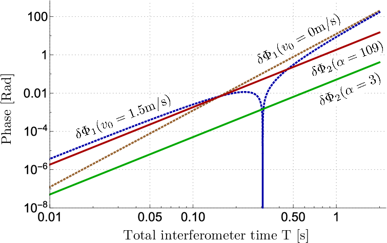
As an illustrative example, we have plotted in Fig. 3 the phase differences in the SG butterfly interferometer induced by the gravitational field. As physical parameters, we take the experimentally feasible values of $m=1.42\times 10^{-25}\text{kg},~g=9.8\text{m}/\text{s}^{2},~\Gamma=mK=3\times 10^{-6}\text{s}^{-2},~\delta v=\delta p/m=0.02\text{m}/\text{s}$ based on Ref. Amit et al. 2019. First of all, the figure shows that when the initial and final positions are the same, only the phase difference from the magnetic moment is nonvanishing. Also, when Rydberg atoms are employed with $\alpha=109$ , the phase difference from the magnetic moment can be large enough to increase the sensitivity.

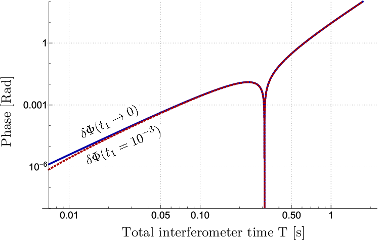
In realistic experiments, the magnetic field in the displacement stage has to be large enough to attain the phase $\delta\Phi$ of the above limit. Taking into account practical situations, we analyze the phase accumulation with a finite time duration of displacement instead of the pulse regime. In this case, from the condition (3), the free evolution time is determined by $T_{f}=t_{1}+2t_{2}$ . We show the phase accumulation from finite time of displacement in Fig. 4. As shown in the figure, the finite time duration for displacement still leads to a phase difference similar to what we obtained in the limit $t_{1}\to 0$ . Since the time duration for displacement is not required to be extremely small, fixing the magnetic moment difference and the momentum difference in Eqs. (14) and (15), one may employ a smaller magnetic-field gradient by increasing $t_{1}$ or $t_{3}$ in practice.

III.3 Visibility

Finally, let us discuss the degradation of the visibility due to the misalignment. The misalignment changes the probabilities of detecting $|1\rangle,|2\rangle$ as $P_{1}=(1+C\cos\delta\Phi)/2$ and $P_{2}=(1-C\cos\delta\Phi)/2$ , where

\displaystyle C=|\langle{\psi_{0}(T)}|\hat{V}^{\dagger}(T)\hat{D}(\Delta z(T),\Delta p(T))\hat{V}(T)|{\psi_{0}(T)}\rangle|

(18)

represents the visibility. Here, $\Delta z(T)=z_{2}(T)-z_{1}(T)$ and $\Delta p(T)=p_{2}(T)-p_{1}(T)$ . Unless $\Delta z(T)=\Delta p(T)=0$ , the visibility of the signal is strictly less than 1. In the butterfly interferometer case with a pulse regime, up to order of $K$ , we have

\displaystyle\Delta z(T)\approx\frac{KT^{3}\delta p}{32m^{2}},~~~~\Delta p(T)\approx 0.

(19)

In the case of Mach-Zehnder type of atomic interferometer, the misalignment is given by

\displaystyle\Delta z(T)\approx\frac{KT^{3}\delta p}{8m^{2}},~~~~\Delta p(T)\approx\frac{KT^{2}\delta p}{4m}.

(20)

To analyze the effect of the misalignment, let us assume the initial wave packet to be Gaussian, with the uncertainty of the position and momentum along the $z$ axis denoted $\sigma_{z}$ and $\sigma_{p_{z}}$ . We assume that the correlation of the position and momentum is zero for simplicity. In this case, the visibility $C$ for a pure state can be simplified as

\displaystyle C=|\langle\psi(0)|\hat{D}(\Delta z^{\prime},\Delta p_{z}^{\prime})|\psi(0)\rangle|=\exp\left[-\frac{\Delta z^{\prime 2}}{8\sigma_{z}^{2}}-\frac{\Delta p_{z}^{\prime 2}}{8\sigma_{p_{z}}^{2}}\right],

(21)

and for a mixed initial state $\hat{\rho}(0)$ ,

\displaystyle C=|\text{Tr}[\hat{D}(\Delta z^{\prime},\Delta p_{z}^{\prime})\hat{\rho}_{0}]|=\exp\left[-\frac{\sigma_{z}^{2}\Delta p_{z}^{\prime 2}+\sigma_{p_{z}}^{2}\Delta z^{\prime 2}}{2\hbar^{2}}\right],

(22)

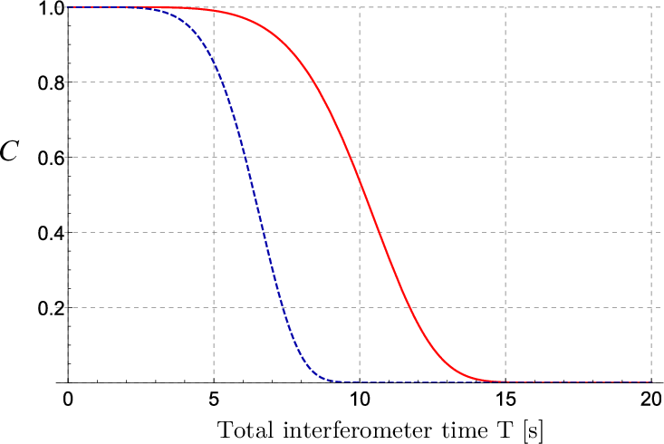
where $\Delta z^{\prime}=\Delta z\cosh\omega T-\frac{\Delta p_{z}}{m\omega}\sinh\omega T$ and $\Delta p_{z}^{\prime}=\Delta p_{z}\cosh\omega T+m\omega\Delta z\sinh\omega T$ . Figure 5 shows the visibility of an example with different interferometer time $T$ . It shows that the visibility is approximately $1$ for $5~\text{seconds}$ and $3~\text{seconds}$ for the butterfly configuration and the Mach-Zehnder type interferometer, respectively. Thus, the butterfly configuration is more robust to the misalignment.

When the visibility is degraded by the misalignment, one may overcome this obstacle by adjusting experimental parameters more elaborately Roura et al. 2014; Roura 2017. For example, for an atomic interferometer based on laser pulses, by changing the frequency of the laser depending on the gravity gradient one can align atoms’ trajectories to reduce the amount of the misalignment. The same technique can be applied by changing the magnetic-field gradient accordingly.

IV Conclusion

We have introduced a variant of a butterfly interferometer that enables a precise measurement of the field gradient. In our SG butterfly configuration, the atoms are prepared in superposition between the internal states having different magnetic moments, so that the external magnetic field can split the trajectories in the time-dependent manner.

The proposed interferometer is flexible in controlling the momentum transfer of the atoms by using the external magnetic field, while it implements the conventional butterfly configuration as a special case. We have shown that the phase difference between the different atomic trajectories arising from the field gradient can be decomposed into magnetic-moment-independent and -dependent parts. The magnetic moment independent phase can be compared with the phase difference in the conventional butterfly interferometer, but can linearly increase by the momentum difference of the interferometer $\delta p$ induced by the external magnetic field. The magnetic-moment-dependent phase provides a distinct feature of the SG butterfly interferometer scaling in $T^{3}$ and can be increased by enlarging the magnetic quantum number of the internal atomic state.

We have also investigated the degradation of the visibility when the interferometer is not perfectly closed due to the field gradient. We have demonstrated that the robustness of the interferometer against the misalignment is comparable to or better than the Mach-Zehnder type of atomic interferometer.

Acknowledgements.

C.O. and L.J. acknowledge support from the ARL-CDQI (W911NF-15-2-0067), ARO (W911NF-18-1-0020, W911NF-18-1-0212), ARO MURI (W911NF-16-1-0349), AFOSR MURI (FA9550-15-1-0015, FA9550-19-1-0399), DOE (DE-SC0019406), NSF (EFMA-1640959, OMA-1936118), and the Packard Foundation (2013-39273). The work of H.K. and M.S.K. was supported by the KIST Open Research Program. M.S.K. acknowledges the visiting professorship at KIAS where this work was initially discussed. The work of M.S.K. was supported by the QuantERA ERA-NET Cofund in Quantum Technologies implemented within the European Union’s Horizon 2020 Programme and EPSRC (EP/R044082/1).

References

Cronin et al. (2009) A. D. Cronin, J. Schmiedmayer, and D. E. Pritchard, “Optics and interferometry with atoms and molecules,” Rev. Mod. Phys. 81, 1051 (2009).
Kasevich and Chu (1991) M. Kasevich and S. Chu, “Atomic interferometry using stimulated raman transitions,” Phys. Rev. Lett. 67, 181 (1991).
Kasevich and Chu (1992) M. Kasevich and S. Chu, “Measurement of the gravitational acceleration of an atom with a light-pulse atom interferometer,” Applied Physics B 54, 321–332 (1992).
Peters et al. (1999) A. Peters, K. Y. Chung, and S. Chu, “Measurement of gravitational acceleration by dropping atoms,” Nature 400, 849–852 (1999).
Fray et al. (2004) S. Fray, C. A. Diez, T. W. Hänsch, and M. Weitz, “Atomic interferometer with amplitude gratings of light and its applications to atom based tests of the equivalence principle,” Phys. Rev. Lett. 93, 240404 (2004).
Müller et al. (2008a) H. Müller, S.-w. Chiow, S. Herrmann, S. Chu, and K.-Y. Chung, “Atom-interferometry tests of the isotropy of post-newtonian gravity,” Phys. Rev. Lett. 100, 031101 (2008a).
Hu et al. (2013) Z.-K. Hu, B.-L. Sun, X.-C. Duan, M.-K. Zhou, L.-L. Chen, S. Zhan, Q.-Z. Zhang, and J. Luo, “Demonstration of an ultrahigh-sensitivity atom-interferometry absolute gravimeter,” Phys. Rev. A 88, 043610 (2013).
Schlippert et al. (2014) D. Schlippert, J. Hartwig, H. Albers, L. L. Richardson, C. Schubert, A. Roura, W. P. Schleich, W. Ertmer, and E. M. Rasel, “Quantum test of the universality of free fall,” Phys. Rev. Lett. 112, 203002 (2014).
Fixler et al. (2007) J. B. Fixler, G. T. Foster, J. M. McGuirk, and M. A. Kasevich, “Atom interferometer measurement of the newtonian constant of gravity,” Science 315, 74–77 (2007).
Lamporesi et al. (2008) G. Lamporesi, A. Bertoldi, L. Cacciapuoti, M. Prevedelli, and G. M. Tino, “Determination of the newtonian gravitational constant using atom interferometry,” Phys. Rev. Lett. 100, 050801 (2008).
Rosi et al. (2014) G. Rosi, F. Sorrentino, L. Cacciapuoti, M. Prevedelli, and G. M. Tino, “Precision measurement of the newtonian gravitational constant using cold atoms,” Nature 510, 518–521 (2014).
Prevedelli et al. (2014) M. Prevedelli, L. Cacciapuoti, G. Rosi, F. Sorrentino, and G. M. Tino, “Measuring the newtonian constant of gravitation g with an atomic interferometer,” Philos. Trans. R. Soc. A 372, 20140030 (2014).
Snadden et al. (1998) M. J. Snadden, J. M. McGuirk, P. Bouyer, K. G. Haritos, and M. A. Kasevich, “Measurement of the earth’s gravity gradient with an atom interferometer-based gravity gradiometer,” Phys. Rev. Lett. 81, 971 (1998).
Mcguirk et al. (2002) J. M. Mcguirk, G. T. Foster, J. B. Fixler, M. J. Snadden, and M. A. Kasevich, “Sensitive absolute-gravity gradiometry using atom interferometry,” Phys. Rev. A 65, 033608 (2002).
Sorrentino et al. (2014) F. Sorrentino, Q. Bodart, L. Cacciapuoti, Y.-H. Lien, M. Prevedelli, G. Rosi, L. Salvi, and G. M. Tino, “Sensitivity limits of a raman atom interferometer as a gravity gradiometer,” Phys. Rev. A 89, 023607 (2014).
Gustavson et al. (1997) T. L. Gustavson, P. Bouyer, and M. A. Kasevich, “Precision rotation measurements with an atom interferometer gyroscope,” Phys. Rev. Lett. 78, 2046 (1997).
Stockton et al. (2011) J. K. Stockton, K. Takase, and M. A. Kasevich, “Absolute geodetic rotation measurement using atom interferometry,” Phys. Rev. Lett. 107, 133001 (2011).
Dutta et al. (2016) I. Dutta, D. Savoie, B. Fang, B. Venon, C. L. Garrido Alzar, R. Geiger, and A. Landragin, “Continuous cold-atom inertial sensor with 1 nrad/sec rotation stability,” Phys. Rev. Lett. 116, 183003 (2016).
Müller et al. (2010) H. Müller, A. Peters, and S. Chu, “A precision measurement of the gravitational redshift by the interference of matter waves,” Nature 463, 926–929 (2010).
Roura (2020) A. Roura, “Gravitational redshift in quantum-clock interferometry,” Phys. Rev. X 10, 021014 (2020).
Parker et al. (2018) R. H. Parker, C. Yu, W. Zhong, B. Estey, and H. Müller, “Measurement of the fine-structure constant as a test of the standard model,” Science 360, 191–195 (2018).
Dimopoulos et al. (2007) S. Dimopoulos, P. W. Graham, J. M. Hogan, and M. A. Kasevich, “Testing general relativity with atom interferometry,” Phys. Rev. Lett. 98, 111102 (2007).
Tarallo et al. (2014) M. G. Tarallo, T. Mazzoni, N. Poli, D. V. Sutyrin, X. Zhang, and G. M. Tino, “Test of Einstein equivalence principle for 0-spin and half-integer-spin atoms: Search for spin-gravity coupling effects,” Phys. Rev. Lett. 113, 023005 (2014).
Hartwig et al. (2015) J. Hartwig, S. Abend, C. Schubert, D. Schlippert, H. Ahlers, K. Posso-Trujillo, N. Gaaloul, W. Ertmer, and E. M. Rasel, “Testing the universality of free fall with rubidium and ytterbium in a very large baseline atom interferometer,” New J. Phys. 17, 035011 (2015).
Zhou et al. (2015) L. Zhou, S. Long, B. Tang, X. Chen, F. Gao, W. Peng, W. Duan, J. Zhong, Z. Xiong, J. Wang, Y. Zhang, and M. Zhan, “Test of equivalence principle at $10^{-8}$ level by a dual-species double-diffraction raman atom interferometer,” Phys. Rev. Lett. 115, 013004 (2015).
Rosi et al. (2017) G. Rosi, G. D’Amico, L. Cacciapuoti, F. Sorrentino, M. Prevedelli, M. Zych, Č. Brukner, and G. M. Tino, “Quantum test of the equivalence principle for atoms in coherent superposition of internal energy states,” Nat. Commun. 8, 1–6 (2017).
Geiger and Trupke (2018) R. Geiger and M. Trupke, “Proposal for a quantum test of the weak equivalence principle with entangled atomic species,” Phys. Rev. Lett. 120, 043602 (2018).
Yang et al. (2012) S.-Q. Yang, B.-F. Zhan, Q.-L. Wang, C.-G. Shao, L.-C. Tu, W.-H. Tan, and J. Luo, “Test of the gravitational inverse square law at millimeter ranges,” Phys. Rev. Lett. 108, 081101 (2012).
Biedermann et al. (2015) G. W. Biedermann, X. Wu, L. Deslauriers, S. Roy, C. Mahadeswaraswamy, and M. A. Kasevich, “Testing gravity with cold-atom interferometers,” Phys. Rev. A 91, 033629 (2015).
Dimopoulos et al. (2008) S. Dimopoulos, P. W. Graham, J. M. Hogan, M. A. Kasevich, and S. Rajendran, “Atomic gravitational wave interferometric sensor,” Phys. Rev. D 78, 122002 (2008).
Graham et al. (2013) P. W. Graham, J. M. Hogan, M. A. Kasevich, and S. Rajendran, “New method for gravitational wave detection with atomic sensors,” Phys. Rev. Lett. 110, 171102 (2013).
Hamilton et al. (2015) P. Hamilton, M. Jaffe, P. Haslinger, Q. Simmons, H. Müller, and J. Khoury, “Atom-interferometry constraints on dark energy,” Science 349, 849–851 (2015).
Sabulsky et al. (2019) D. O. Sabulsky, I. Dutta, E. A. Hinds, B. Elder, C. Burrage, and E. J. Copeland, “Experiment to detect dark energy forces using atom interferometry,” Phys. Rev. Lett. 123, 061102 (2019).
Bose et al. (2017) S. Bose, A. Mazumdar, G. W. Morley, H. Ulbricht, M. Toroš, M. Paternostro, A. A. Geraci, P. F. Barker, M. S. Kim, and G. Milburn, “Spin entanglement witness for quantum gravity,” Phys. Rev. Lett. 119, 240401 (2017).
Marletto and Vedral (2017) C. Marletto and V. Vedral, “Gravitationally induced entanglement between two massive particles is sufficient evidence of quantum effects in gravity,” Phys. Rev. Lett. 119, 240402 (2017).
McGuirk et al. (2000) J. M. McGuirk, M. J. Snadden, and M. A. Kasevich, “Large area light-pulse atom interferometry,” Phys. Rev. Lett. 85, 4498 (2000).
Müller et al. (2008b) H. Müller, S.-w. Chiow, Q. Long, S. Herrmann, and S. Chu, “Atom interferometry with up to 24-photon-momentum-transfer beam splitters,” Phys. Rev. Lett. 100, 180405 (2008b).
Cladé et al. (2009) P. Cladé, S. Guellati-Khélifa, F. Nez, and F. Biraben, “Large momentum beam splitter using bloch oscillations,” Phys. Rev. Lett. 102, 240402 (2009).
Chiow et al. (2011) S.-w. Chiow, T. Kovachy, H.-C. Chien, and M. A. Kasevich, “102 $\hbar k$ large area atom interferometers,” Phys. Rev. Lett. 107, 130403 (2011).
Asenbaum et al. (2017) P. Asenbaum, C. Overstreet, T. Kovachy, D. D. Brown, J. M. Hogan, and M. A. Kasevich, “Phase shift in an atom interferometer due to spacetime curvature across its wave function,” Phys. Rev. Lett. 118, 183602 (2017).
Kovachy et al. (2015) T. Kovachy, P. Asenbaum, C. Overstreet, C. A. Donnelly, S. M. Dickerson, A. Sugarbaker, J. M. Hogan, and M. A. Kasevich, “Quantum superposition at the half-metre scale,” Nature 528, 530–533 (2015).
Gerlach and Stern (1922) W. Gerlach and O. Stern, “Der experimentelle nachweis der richtungsquantelung im magnetfeld,” Zeitschrift für Physik 9, 349–352 (1922).
Bohm (2012) D. Bohm, Quantum theory (Courier Corporation, 2012).
Wigner (1963) E. P. Wigner, “The problem of measurement,” Am. J. Phys. 31, 6–15 (1963).
Machluf et al. (2013) S. Machluf, Y. Japha, and R. Folman, “Coherent Stern-Gerlach momentum splitting on an atom chip,” Nat. Commun. 4, 1–9 (2013).
Zimmermann et al. (2017) M. Zimmermann, M. Efremov, A. Roura, W. Schleich, S. DeSavage, J. Davis, A. Srinivasan, F. Narducci, S. Werner, and E. Rasel, “ ${T}^{3}$ -interferometer for atoms.” Applied Physics B: Lasers & Optics 123, 102 (2017).
Margalit et al. (2018) Y. Margalit, Z. Zhou, O. Dobkowski, Y. Japha, D. Rohrlich, S. Moukouri, and R. Folman, “Realization of a complete Stern-Gerlach interferometer,” arXiv preprint arXiv:1801.02708 (2018).
Amit et al. (2019) O. Amit, Y. Margalit, O. Dobkowski, Z. Zhou, Y. Japha, M. Zimmermann, M. A. Efremov, F. A. Narducci, E. M. Rasel, W. P. Schleich, and R. Folman, “ ${T}^{3}$ Stern-Gerlach matter-wave interferometer,” Phys. Rev. Lett. 123, 083601 (2019).
Margalit et al. (2019) Y. Margalit, Z. Zhou, S. Machluf, Y. Japha, S. Moukouri, and R. Folman, “Analysis of a high-stability Stern–Gerlach spatial fringe interferometer,” New J. Phys. 21, 073040 (2019).
Englert et al. (1988) B.-G. Englert, J. Schwinger, and M. O. Scully, “Is spin coherence like humpty-dumpty? i. simplified treatment,” Foundations of physics 18, 1045–1056 (1988).
Schwinger et al. (1988) J. Schwinger, M. O. Scully, and B.-G. Englert, “Is spin coherence like humpty-dumpty?” Zeitschrift für Physik D Atoms, Molecules and Clusters 10, 135–144 (1988).
Scully et al. (1989) M. O. Scully, B.-G. Englert, and J. Schwinger, “Spin coherence and humpty-dumpty. iii. the effects of observation,” Phys. Rev. A 40, 1775 (1989).
Comparat (2020) D. Comparat, “Limitations for field-enhanced atom interferometry,” Phys. Rev. A 101, 023606 (2020).
Damour and Polyakov (1994) T. Damour and A. M. Polyakov, “The string dilaton and a least coupling principle,” Nuclear physics. B 423, 532–558 (1994).
Butler (1984) D. K. Butler, “Microgravimetric and gravity gradient techniques for detection of subsurface cavities,” Geophysics 49, 1084–1096 (1984).
Mikhailov et al. (2007) V. Mikhailov, G. Pajot, M. Diament, and A. Price, “Tensor deconvolution: A method to locate equivalent sources from full tensor gravity data,” Geophysics 72, I61–I69 (2007).
Lawrence (2012) A. Lawrence, Modern inertial technology: navigation, guidance, and control (Springer Science & Business Media, 2012).
Romaides et al. (2001) A. J. Romaides, J. C. Battis, R. W. Sands, A. Zorn, D. O. Benson Jr, and D. J. DiFrancesco, “A comparison of gravimetric techniques for measuring subsurface void signals,” J. Phys. D Appl. Phys. 34, 433 (2001).
Fischbach et al. (1986) E. Fischbach, D. Sudarsky, A. Szafer, C. Talmadge, and S. H. Aronson, “Reanalysis of the eoumltvös experiment,” Phys. Rev. Lett. 56, 3 (1986).
Roura et al. (2014) A. Roura, W. Zeller, and W. P. Schleich, “Overcoming loss of contrast in atom interferometry due to gravity gradients,” New J. Phys. 16, 123012 (2014).
D’Amico et al. (2017) G. D’Amico, G. Rosi, S. Zhan, L. Cacciapuoti, M. Fattori, and G. M. Tino, “Canceling the gravity gradient phase shift in atom interferometry,” Phys. Rev. Lett. 119, 253201 (2017).
Clauser (1988) J. F. Clauser, “Ultra-high sensitivity accelerometers and gyroscopes using neutral atom matter-wave interferometry,” Physica B+ C 151, 262–272 (1988).
Marzlin and Audretsch (1996) K.-P. Marzlin and J. Audretsch, “State independence in atom interferometry and insensitivity to acceleration and rotation,” Phys. Rev. A 53, 312 (1996).
Canuel et al. (2006) B. Canuel, F. Leduc, D. Holleville, A. Gauguet, J. Fils, A. Virdis, A. Clairon, N. Dimarcq, C. J. Bordé, A. Landragin, and P. Bouyer, “Six-axis inertial sensor using cold-atom interferometry,” Phys. Rev. Lett. 97, 010402 (2006).
Dubetsky and Kasevich (2006) B. Dubetsky and M. A. Kasevich, “Atom interferometer as a selective sensor of rotation or gravity,” Phys. Rev. A 74, 023615 (2006).
Wu et al. (2007) S. Wu, E. Su, and M. Prentiss, “Demonstration of an area-enclosing guided-atom interferometer for rotation sensing,” Phys. Rev. Lett. 99, 173201 (2007).
Tonyushkin and Prentiss (2008) A. Tonyushkin and M. Prentiss, “Selective manipulation of degenerate interferometer loops by an atom-optics kicked rotor,” Phys. Rev. A 78, 053625 (2008).
Takase (2008) K. Takase, Precision rotation rate measurements with a mobile atom interferometer, Ph.D. thesis, Stanford University (2008).
Kleinert et al. (2015) S. Kleinert, E. Kajari, A. Roura, and W. P. Schleich, “Representation-free description of light-pulse atom interferometry including non-inertial effects,” Physics Reports 605, 1–50 (2015).
Zimmermann et al. (2019) M. Zimmermann, M. A. Efremov, W. Zeller, W. P. Schleich, J. P. Davis, and F. A. Narducci, “Representation-free description of atom interferometers in time-dependent linear potentials,” New J. Phys. 21, 073031 (2019).
Palmer and Hogan (2019) J. E. Palmer and S. D. Hogan, “Electric rydberg-atom interferometry,” Phys. Rev. Lett. 122, 250404 (2019).
Roura (2017) A. Roura, “Circumventing heisenberg’s uncertainty principle in atom interferometry tests of the equivalence principle,” Phys. Rev. Lett. 118, 160401 (2017).