General relativistic MHD simulations of non-thermal flaring in Sagittarius A*2019General relativistic MHD simulations of non-thermal flaring in Sagittarius A*–A
Abstract
Sgr A∗ exhibits regular variability in its multiwavelength emission, including daily X-ray flares and roughly continuous near-infrared (NIR) flickering. The origin of this variability is still ambiguous since both inverse Compton and synchrotron emission are possible radiative mechanisms. The underlying particle distributions are also not well constrained, particularly the non-thermal contribution. In this work, we employ the GPU-accelerated general relativistic magnetohydrodynamics (GRMHD) code H-AMR to perform a study of flare flux distributions, including the effect of particle acceleration for the first time in high-resolution 3D simulations of Sgr A∗. For the particle acceleration, we use the general relativistic ray-tracing (GRRT) code BHOSS to perform the radiative transfer, assuming a hybrid thermalnon-thermal electron energy distribution. We extract hr lightcurves in the sub-millimetre, NIR and X-ray wavebands, and compare the power spectra and the cumulative flux distributions of the lightcurves to statistical descriptions for Sgr A∗ flares. Our results indicate that non-thermal populations of electrons arising from turbulence-driven reconnection in weakly magnetised accretion flows lead to moderate NIR and X-ray flares and reasonably describe the X-ray flux distribution while fulfilling multiwavelength flux constraints. These models exhibit high rms% amplitudes, both in the NIR and the X-rays, with changes in the accretion rate driving the 230 GHz flux variability, in agreement with Sgr A∗ observations.
Keywords:
galaxies: black hole physics – accretion, accretion discs, jets – galaxies: individual (Milky Way: Sgr A∗) – magnetohydrodynamics (MHD) – methods: numerical1 Introduction
The extreme physical conditions in the vicinity of accreting black holes (BHs) present a unique opportunity to study the acceleration of particles in conditions unattainable on Earth. Magnetised plasma turbulence, instabilities, and shocks occurring naturally in accretion flows and outflows are all potential processes that trigger particle acceleration. Sagittarius A∗ (Sgr A∗), the supermassive BH (SMBH) candidate at the centre of our galaxy, due to its proximity, presents an excellent opportunity to test current theories about particle acceleration near BHs against high-quality observational data. Intensive monitoring of Sgr A∗ has led to accurate measurements of stellar orbits yielding a BH mass of (Ghez et al. 2005; Gillessen et al. 2017; Gravity Collaboration et al. 2018a) at a distance of kpc (Ghez et al. 2008; Boehle et al. 2016; Reid et al. 2019, e.g.,) from the Earth, and resulted in a systematic study of its emission in the radio, millimetre (mm), near-infrared (NIR) and X-ray wavebands (e.g., see Genzel et al. 2010, and references therein). Sgr A∗ is a remarkably faint SMBH (luminosity , where is the Eddington luminosity) that accretes gas at an estimated rate of yr-1 (Bower et al. 2003; Marrone et al. 2007; Wang et al. 2013). Almost % of the accreted gas at the Bondi scale is lost due to turbulence and/or outflows by the time the flow reaches the black hole (Wang et al. 2013). At such a low accretion rate the accretion flow can be expected to be radiatively inefficient (e.g., Yuan et al. 2003; also see Yuan & Narayan 2014 and references therein). In spite of its low luminosity, Sgr A∗ is one of our best opportunities to study a SMBH via its interaction with accreting material, and it plays a crucial role in our understanding of extreme gravitational environments.
Observations at multiple wavelengths over the previous two decades have constrained the quiescent spectrum of Sgr A∗. In the sub-millimetre (sub-mm) band, Bower et al. 2019 found a spectral index of (where the flux density is ) with the peak flux lying between 1 and 2 terahertz. Using a thermal synchrotron emission model to account for both the sub-mm and the NIR flux, Bower et al. 2019 estimates an electron temperature of K along with a small magnetic field strength of G in the inner accretion flow, consistent with previous semi-analytic results (Falcke et al. 2000; Markoff et al. 2001; Yuan et al. 2002, e.g.,). In the quiescent state, the X-rays seem to be dominated by thermal bremsstrahlung from the Bondi-scale accretion flow (Quataert 2002; Baganoff et al. 2003; Yuan et al. 2003, e.g.,).
Apart from its low-luminosity quiescent state, Sgr A∗ regularly displays fluctuations in flux across multiple frequencies, most prominently in the NIR and X-ray bands, which are often correlated with each other (Eckart et al. 2004; Dodds-Eden et al. 2009; Boyce et al. 2019, e.g.,). Ever since Baganoff et al. 2001 reported the first detection of an X-ray flaring event in Sgr A∗ with the Chandra X-ray Observatory, the SMBH has been the target of multiple observational campaigns (e.g., the 3 Ms 2012 Chandra X-ray Visionary Project11 1 http://www.sgra-star.com and the Neil Gehrels Swift Observatory22 2 https://swift.gsfc.nasa.gov monitoring campaign; Degenaar et al. 2015). In 2019, Do et al. 2019 and Haggard et al. 2019 reported the largest flares yet detected from Sgr A∗ at 2.12 m (NIR) with the Keck Telescope and in the 2-8 keV energy band (X-ray) with Chandra, respectively. Further, NuSTAR observations confirmed that Sgr A∗’s X-ray flares have higher energy extensions (Barrière et al. 2014, e.g.,) with a luminosity of erg s-1 and photon index (Zhang et al. 2017) similar to the 2-8 keV Chandra Nowak et al. 2012 photon index (). The X-ray emission of Sgr A∗ is the lowest among observed low-luminosity SMBHs, allowing the detection of low-flux stochastic flaring events in the innermost regions of the accretion flow. It is still an open question of whether this is due to the absence of a pronounced jet feature that usually dominates the X-ray emission in other accreting SMBHs. The immense amount of observational data allows us to investigate these pivotal questions about the plasma conditions in Sgr A∗.
Most semi-analytical studies are agnostic about the exact mechanism behind particle acceleration in Sgr A∗ (Quataert & Narayan 1999; Özel et al. 2000; Markoff et al. 2001; Liu & Melia 2001; Yuan et al. 2003; Markoff 2005; Li et al. 2015; Connors et al. 2017, e.g.,), whether it be from shocks or magnetic reconnection. Non-thermal synchrotron emission is generally favoured over synchrotron-self-Compton (SSC) to be the source of simultaneous NIR and X-ray flaring events since only a few local parameters, such as the acceleration efficiency or the power-law index, need to change in order to transition from the quiescent phase to a flare state (Dibi et al. 2014, e.g.,). Additionally, when simultaneous NIR/X-ray flares are observed the required steepening of the slope between these bands is a challenge to fit with SSC models but fits expectations for a cooling break in synchrotron radiation (Markoff et al. 2001; Dodds-Eden et al. 2009; Dodds-Eden et al. 2010; Dibi et al. 2014; Ponti et al. 2017, e.g.,). For SSC flare models, Dibi et al. 2014 showed that flares can only occur if the accretion rate and/or the global magnetic field strength changes. However, the low radio and sub-mm flux variability may rule out large changes in the accretion rate during observed flaring states. With more simultaneous NIR/X-ray surveys, such as Boyce et al. 2019, flare flux distributions provide the potential to statistically differentiate between synchrotron and SSC models.
Flare flux probability distribution functions (PDFs) are a useful tool to understand the possible physical mechanisms behind NIR versus X-ray flaring, without requiring individual fits to the properties of individual flares such as flare duration, shape and time delays. The NIR cumulative distribution function (CDF) consists of a log-normal component that captures the low-flux distribution (Witzel et al. 2012; Witzel et al. 2018) with an additional power-law for the high fluxes (Dodds-Eden et al. 2010). In this paper, we take the CDF from Do et al. 2019, where in addition to the log-normal component from Witzel et al. 2018, there is a power-law tail with index . However, we should note here that the power-law index is still debated as Dodds-Eden et al. 2010 found an index of while Witzel et al. 2012 and Witzel et al. 2018 found a steep index of 33 3 Some of these papers actually quote the slope of the flux PDFs instead of the CDFs. For a power-law, the slope is reduced by 1 when transforming from the PDF to the CDF.. The X-ray CDF can be modelled as a Poissonian with a power-law tail (Neilsen et al. 2015). The power-law index for the NIR CDF is , which is close to the Do et al. 2019 NIR CDF slope. Taking the Witzel et al. 2012 NIR CDF slope of 3.2 and the Neilsen et al. 2015 X-ray CDF slope of 1.92, Dibi et al. 2016 shows that the large difference between the slopes of NIR and X-ray cumulative distribution functions is not well described by simpler synchrotron scenarios and leaves the door open for a fuller exploration of models involving both SSC from a thermal electron population and synchrotron from a non-thermal electron population. Hence, further studies of the relation of the NIR and X-ray CDF slope is required to disentangle common processes that could give rise to both flare populations.
The origin of large NIR flares such as the one reported in Do et al. 2019 is still unknown. In Do et al. 2019, the authors suggest that an increase in the accretion rate could explain the exceptionally high flux. Unfortunately, simultaneous observations at sub-mm are not available to confirm this theory. As an alternative to a change in the accretion rate, Gutiérrez et al. 2020 demonstrates that large NIR flares could have a non-thermal origin in the form of a magnetised blob of plasma, i.e., a plasmoid. Local particle-in-cell simulations show that plasmoids can naturally form as a result of relativistic magnetic reconnection in environments that are prevalent in accretion discs as well as the jet boundary (Sironi et al. 2015; Ball et al. 2018; Hakobyan et al. 2019, e.g.,), but whether such plasmoids grow to the sizes required to explain the enormous flux is not yet known. The computational demands of these simulations prohibit the exploration of bulk flow effects on the microscopic plasmoid behaviour, requiring alternate schemes to incorporate the global turbulence of the accretion flows.
The idea that plasmoids are responsible for NIR flaring gained even more traction with the Gravity Collaboration et al. 2018b detection of three NIR flares consistent with hotspots orbiting at a distance of gravitational radii (, where and are the gravitational constant and the speed of light respectively) from the BH with an inclination of approximately degrees and an orbital period minutes (Gravity Collaboration et al. 2020b). This detection points towards localised mechanisms such as magnetic reconnection and electron heating behind the NIR flaring, indicating the need to understand the small-scale activity of the accretion flow via numerical simulations (Dexter et al. 2020b; Porth et al. 2021, e.g., see).
Over the past decades, the theoretical astrophysics community has increasingly used general relativistic magnetohydrodynamic (GRMHD) simulations of accreting BHs to produce a more self-consistent description of accretion dynamics. GRMHD simulations usually employ the single fluid approximation, assuming that the ion temperature dominates the flow temperature and that the ions are in a thermal distribution. With the additional simplifying assumption of neutral hydrogen, we assume each proton is accompanied by an electron. Therefore, we require a model that describes the electron temperature in postprocessing (Howes 2010; Rowan et al. 2017; Werner et al. 2018, e.g.,). Along with GRMHD quantities, the choice of the electron temperature model is important to generate multiwavelength spectra using general relativistic ray-tracing (GRRT) codes, and thus, enable us to compare simulated data to the observed spectrum of Sgr A∗ (Dexter et al. 2009; Mościbrodzka et al. 2009; Dexter et al. 2010; Dibi et al. 2012; Shcherbakov et al. 2012; Drappeau et al. 2013; Mościbrodzka & Falcke 2013; Chan et al. 2015; Mao et al. 2017; Davelaar et al. 2018; Anantua et al. 2020, e.g.,). A computationally more expensive alternative approach is to evolve the electron thermodynamics along with the gas evolution self-consistently within a GRMHD simulation (Ressler et al. 2015; Ryan et al. 2017; Chael et al. 2018; Dexter et al. 2020a; Mizuno et al. 2021, e.g.,).
Using the robust framework of GRMHDGRRT methods (Porth et al. 2019; Gold et al. 2020, e.g.,), quite a few studies have tried to investigate the properties of the accretion flow that lead to flares. The 2D GRMHD simulations in Drappeau et al. 2013 consider thermal SSC origins of X-ray flaring. Chan et al. 2015 was the first to use 3D GRMHD simulations that invoke thermal bremsstrahlung emission to model undetected X-ray flares (Neilsen et al. 2013, of the quiescent X-ray flux;), thought to come from the inner accretion flow. Further, Ball et al. 2016 and Mao et al. 2017 used a hybrid thermal+non-thermal synchrotron model (Özel et al. 2000) while Davelaar et al. 2018 employed a -distribution model to study Sgr A∗’s X-ray emission. However, the 2D restriction and/or the relatively low resolution of these simulations might result in spurious numerical artefacts. Indeed, Dexter et al. 2020b and Porth et al. 2021 employed high resolution 3D GRMHD simulations to argue that magnetically saturated BHs release small scale magnetic eruptions leading to the formation of orbiting NIR features, a possible mechanism to explain GRAVITY-observed flares. Porth et al. 2021 found that the observed hotspots orbit faster than the simulated NIR features, hinting at super-Keplerian motions (Matsumoto et al. 2020, e.g.,). Although these GRMHD studies restrict their scope to reconnection features in the disc, possible NIR flare models do not yet preclude outflowing features. Outflowing magnetic reconnection zones at wind or jet boundaries, when viewed in projection (Nathanail et al. 2020; Ripperda et al. 2020; Ball et al. 2021, e.g.,), could appear to move as the observed hotspots, despite the apparent absence of a well-collimated outflow in Sgr A∗ (Markoff et al. 2007; Issaoun et al. 2019, though the size constraints of the central sub-mm source might allow for a jet; e.g., see). The highly anticipated results of the Event Horizon Telescope (Doeleman et al. 2008; EHTC et al. 2019a) observations of Sgr A∗ promise to reveal much more about the horizon-scale structure and add to the plethora of observational data. Despite the recent advances made in modelling flares, no 3D high resolution GRMHD simulation has yet tackled the inconsistency of Sgr A∗’s NIR/Xray flare flux distribution slopes raised in Dibi et al. 2016 and whether turbulence-driven non-thermal activity can explain the overall behaviour of NIR and X-ray flares.
To address these questions, we employ the state-of-the-art GPU-accelerated GRMHD code H-AMR (Liska et al. 2019) to simulate BH accretion discs and jets, together with the GRRT code BHOSS (Younsi et al. 2020) to generate synchrotron-only spectra assuming a hybrid thermal+non-thermal electron distribution, and do not account for inverse Compton scattering. For the first time, we evolve fully 3D simulations at high resolutions to calculate Sgr A∗ lightcurves over a significantly long time period to study the role of disc and jet turbulence in determining the observed flux variability. The long lightcurves thus produced also provide a key perspective beyond spectral properties. To that end we extract NIR/X-ray flare statistics from the simulations, providing a view of GRMHD BH discs complementary to other recent theoretical papers that focus on magnetised features to explain the NIR flaring (Dexter et al. 2020b; Gutiérrez et al. 2020; Petersen & Gammie 2020; Porth et al. 2021; Ball et al. 2021, e.g.,). For the NIR/X-ray flare statistics, we primarily focus on comparing cumulative flux distributions both in the NIR (Do et al. 2019) and the X-rays (Neilsen et al. 2015), restricting our analysis to the inner accretion flow (within ) that has marginally reached inflow equilibrium (Narayan et al. 2012, using the criteria given in). We provide a detailed overview of our numerical methods in Sec. 2 and 3, present and discuss our results in Sec. 4 and 5, and subsequently, conclude in Sec. 6.
| GRMHD parameters |
| Model | a | Resolution | |||
| () | [] | [] | [] | ||
| All | 0.9375 | 12.5 | 25 |
| Model | B-flux | -factor | ||
|---|---|---|---|---|
| strength | [ | |||
| Weak | Weak-field | 3.8 | (7.1, 8.1, 29.5) | 2.93 |
| Strong | Strong-field | 39.7 | 34.5, 26.1, 85.4) | 3.34 |
| GRRT parameters |
| Model | FOV | Image | Sgr A∗ & | Inclination |
|---|---|---|---|---|
| [] | resolution | [, kpc] | [degrees] | |
| All | , |
| Model | Accretion rate | ||||
|---|---|---|---|---|---|
| [ yr-1] | |||||
| Weak | 10 | 10 | |||
| Strong | 40 | 10 |
2 Simulation setup
H-AMR (Liska et al. 2018; Chatterjee et al. 2019; Porth et al. 2019; Liska et al. 2019) evolves the GRMHD equations set in a fixed Kerr spacetime, specifically in logarithmic Kerr-Schild (KS) coordinates. H-AMR makes use of advanced techniques such as adaptive mesh refinement (AMR), static mesh de-refinement, local adaptive time-stepping and a staggered mesh setup for evolving the magnetic field (see Liska et al. 2019 for more details about these methods, and Porth et al. 2019 for comparisons to results from other current GRMHD codes for a standard BH accretion disc problem). We adopt the geometrical unit convention, taking , and normalise our length scale to the gravitational radius . The GRMHD simulation grid is axisymmetric, logarithmically-spaced in , and uniform in and , and extends from to . We use static mesh de-refinement to reduce the number of cells in around the polar axis by a factor of 2 (similar to Liska et al. 2018, but without stretching the polar cells in ). We did not make use of AMR in this work. We take the BH spin parameter to be and therefore, our inner radial boundary is inside the event horizon radius (). The grid resolution is . The resolution in sufficiently resolves moderately thick discs (Porth et al. 2019, scale height near the BH;) with 5-13 cells. We use outflowing radial boundary conditions (BCs), transmissive polar BCs (Liska et al. 2018, see supplementary information in) and periodic -BCs.
The accretion disc is set up in the form of the standard Fishbone & Moncrief 1976 hydrostatic torus rotating around the spinning BH (refer to Table 1 for torus and other model specifications). A non-relativistic ideal gas equation of state is assumed: the gas pressure , where and is the internal energy. We perform two simulations, one that leads to a weak jet (model Weak) and the other a relatively strong jet (model Strong). We assume a single poloidal loop in the initial disc magnetic field configuration for both simulations, indicated by the magnetic vector potential ():
where is the rest-mass gas density in code units. The magnetic field strength in the initial condition is normalised by setting , where is the magnetic pressure in Heaviside-Lorentz units and is the co-moving magnetic field strength. Solving the GRMHD equations provides the gas density, internal energy, velocities and magnetic field components per grid cell. Assuming a hydrogen-only, electron-proton plasma, protons dominate the gas density and internal energy, and therefore, we need to assume an electron distribution function and temperature in postprocessing.
The grid resolution is the same for both simulations and is sufficient to resolve the magnetorotational instability (Balbus & Hawley 1991, MRI;) in the disc. We use the standard MRI quality factors to measure the number of cells resolving the largest MRI wavelength, volume-averaged over the disc (using the gas density as the weight in the average; Chatterjee et al. 2020). In the definition of , , and are the Alfvén speed in the -th direction, the corresponding cell size and the fluid angular velocity, respectively. While we adequately resolve the MRI in model Strong with values above 25 (Hawley et al. 2011; Porth et al. 2019, a minimum of 10 is usually quoted for convergence of disc parameters, see), model Weak is only marginally resolved due to weaker magnetic fields in the disc. A brief summary of the simulation details is given in Table 1.
Current grid codes are prone to numerical errors when solving the GRMHD equations for gas density and internal energy within the vacuous jet funnel. These errors are due to gas either being expelled as an outflow or accreted via the BH’s gravity, leaving behind a vacuum region with extremely high magnetisations that GRMHD codes fail to deal with, hence requiring the use of an ad-hoc density floor model. We set a minimum gas density limit of and a minimum internal energy limit of , mass-loading the jet funnel according to the implementation described in Ressler et al. 2017. Gas thermodynamics is unreliable in the jet funnel since small errors in propagate as large errors in internal energy due to the huge scale separation between magnetic and thermal energies. Therefore, we do not account for any emission coming the jet, which we define as regions with , where is the magnetisation.
3 Radiative transfer model
In this section, we describe our model for the electron distribution function, using the general relativistic ray-tracing (GRRT) code BHOSS (Younsi et al. 2012; Younsi et al. 2016; Younsi et al. 2020) to calculate the corresponding synchrotron emission. We generate multiwavelength images and spectra of both simulations (scaled to the mass and distance of Sgr A∗) at a cadence of , accounting for all emission within only. We employ a hybrid thermalnon-thermal electron distribution, assuming two different acceleration models for the non-thermal synchrotron emission. In order to speed up our GRRT calculations, we make use of fitting functions for the synchrotron emissivity and absorption of a relativistic thermal Maxwell-Jüttner distribution from Leung et al. 2011 and a non-thermal power-law distribution from Fouka & Ouichaoui 2014 (see Appendix A for more details).
3.1 Thermal synchrotron modelling
First, we calculate the electron temperature via the Mościbrodzka et al. 2016 prescription based on turbulent heating models that gives us the ion-electron temperature ratio () in the form,
| (7) |
where is the plasma-, defined as the ratio of the gas and magnetic pressures. Plasma- varies both in time and space with typically large values in the disc and small in the jet. Assuming that the contribution of the electrons to the total gas pressure is negligible, we can calculate the electron temperature as:
| (8) |
where and are the proton mass and the Boltzmann constant respectively. We adopt and values for each simulation model such that we are able produce an average spectrum which resembles Sgr A∗’s sub-mm to NIR spectrum. The specific values of and are given in Table 1. Using the electron temperature prescription, we can calculate the thermal synchrotron spectrum from our GRMHD models.
The total thermal energy density is given by,
| (9) |
where is the total thermal electron number density. Here, is the dimensionless electron temperature with as the electron mass. Gammie & Popham 1998 gives in a simplified form,
| (10) |
The expression for gives us the thermal energy density for small , i.e., non-relativistic temperatures, and for large relativistic temperatures.
3.2 Non-thermal synchrotron modelling
We consider a simple non-thermal synchrotron model where electrons are accelerated via magnetic dissipation, inspired by the early hybrid thermalnon-thermal model of Özel et al. 2000. Such a treatment for the electron distribution function is similar to several other prior works, e.g., Markoff et al. 2001; Broderick & McKinney 2010; Dexter et al. 2012; Mao et al. 2017; Connors et al. 2017. In practice, we take a portion of the available thermal electron population and create a non-thermal population with a given total energy density. The co-moving energy density in the non-thermal population () is given by,
| (11) |
where we have a power-law distribution . Here, is the electron Lorentz factor, is the power-law distribution index, and and are the maximum and minimum electron Lorentz factors in the distribution respectively. We tie to the peak of the Maxwellian distribution44 4 We note that other authors have used the condition to smoothly connect the thermal and non-thermal distributions and calculate (Özel et al. 2000; Yuan et al. 2003; Mao et al. 2017, e.g.,).:
| (12) |
which provides a physical normalisation for the power-law since PIC simulations demonstrate that electrons accelerate out of the thermal pool. We set to be
| (13) |
Markoff et al. 2001 found that is required to explain the Baganoff et al. 2001 X-ray flare, thus motivating an assumed of to achieve large X-ray fluxes in regions with high electron temperatures.
Next, instead of a single power-law, we include synchrotron cooling (refer to Appendix Eqn. (38)) by calculating the break Lorentz factor . To get for a particular cell, we equate the local synchrotron cooling timescale to the advection timescale as follows:
| (14) |
Here, and are the bulk fluid radial velocity and the Thomson cross-section, while the electron velocity . Synchrotron cooling is crucial for our analysis since previous semi-analytical work such as Dodds-Eden et al. 2009 has shown that a broken power-law is necessary explain simultaneous NIR/X-ray flares with synchrotron.
In highly magnetised regions, we accelerate electrons out of the thermal pool to a power-law distribution using two different injection models and calculate the radiative output of each GRMHD model (see Table 1).
3.2.1 Constant power-law injection: model
Our first acceleration model assumes that the total non-thermal electron energy density is a fraction of the available magnetic field energy (Broderick & McKinney 2010; Dexter et al. 2012, e.g.,). We assume a constant injected power-law index of
| (15) |
motivated by both observations (Nowak et al. 2012, e.g.,) and semi-analytical modelling (Connors et al. 2017, e.g.,) of Sgr A∗. Since we expect efficient particle acceleration to occur in magnetically dominated regions, we use a criterion for the acceleration efficiency that promotes non-thermal activity in regions where the magnetic energy dominates over the rest-mass energy, i.e., where (Broderick & McKinney 2010). Keeping our criterion in mind, we assume a total non-thermal energy density:
| (16) |
The above equation, combined with Eqn. (11), gives us the non-thermal electron number density for each grid cell, and captures changes in the magnetic energy density that might lead to NIR and X-ray variability, given a constant efficiency coefficient . As Broderick & McKinney 2010 state, Eqn. (16) reduces to in highly magnetised zones. We note that the reduced form of Eqn. (16) is the same as that employed in Dexter et al. 2012, where the authors considered the jet launching region in M87. Particle-in-cell (PIC) simulations provide a self-consistent explanation of the generation of non-thermal activity by resolving the formation and evolution of plasmoids within current sheets using a fully kinetic framework (Sironi & Spitkovsky 2014; Guo et al. 2014; Werner et al. 2018; Ball et al. 2018, e.g.,). In the next section, we describe a PIC-motivated radiation model.


3.2.2 Varying power-law injection: model
In the previous section, we relied on a physically motivated ad-hoc prescription for the acceleration efficiency and a constant power-law index, remaining agnostic about the accelerating process. In the case of magnetic reconnection, PIC simulations suggest that both of these quantities are dependent on the surrounding conditions, such as plasma- and the magnetisation () (e.g., Werner et al. 2018; Ball et al. 2018, and references therein), especially in the trans-relativistic regime (i.e., ). Current 3D GRMHD simulations lack the resolution required to resolve the small-scale structure of plasmoids, or magnetised blobs of gas, that form as a result of magnetic reconnection in current sheets. Only recently have we seen plasmoid evolution in high resolution 2D GRMHD simulations (Nathanail et al. 2020; Ripperda et al. 2020). While it is conceivable that current sheets may be resolvable using advanced simulation grids such as adaptive meshes, for this study, we rely on current sheets and particle acceleration prescriptions from PIC parameter surveys to generate the variability seen in the X-ray emission of Sgr A∗.
We incorporate the non-thermal electron acceleration prescriptions for magnetic reconnection given by Ball et al. 2018. Davelaar et al. 2019 used the same acceleration prescriptions to incorporate non-thermal particles in their simulations of M87. The primary difference in our approach is that whereas Davelaar et al. 2019 employed the use of the relativistic distribution function (Xiao 2006), applying only the power-law index prescription of Ball et al. 2018, we calculate the thermal and non-thermal components of the synchrotron emission separately and account for both PIC-motivated power-law indices and efficiencies. Such an approach removes two degrees of freedom from our first radiative scheme.
Ball et al. 2018 tracks the evolution of the non-thermal electron distribution in a reconnecting layer embedded in an ambient plasma- and magnetisation (hereafter referred to as and ). For our simulations, we calculate the ambient values for each cell in the entire simulation grid by taking the average over the nearest 2 cells in each direction as follows:
| (17) | ||||
| (18) |
In our simulations, current sheets would appear in the disc/sheath as regions with small values of (i.e., regions where magnetic fields reconnect and the field strength drops) encapsulated by regions of large (Ripperda et al. 2020, e.g.,). A grid cell with large values of and would presumably contain a current sheet within it and should exhibit a power-law tail in the electron distribution.
Ball et al. 2018 gives the power-law electron distribution slope and the non-thermal acceleration efficiency in terms of and :
| (19) |
where , , , and,
| (20) |
Since the total electron number density is (, the total proton number density, due to charge neutrality), we can simplify the efficiency as,
| (21) |
where is the peak Lorentz factor of the Maxwellian distribution. To simplify the thermal case, we have chosen the minimum limit of the integration over to be rather than , which gives a simpler analytical form for the total thermal energy density shown in Eqn. (9). This assumption for the integral limits for the thermal electron energy density results in a larger population of electrons being accelerated to a power-law in high temperature regions as compared to what we expect from Eqn. (21). However, note that Eqn. (20) is not strictly the same as Eqn. (21) since the numerator in Eqn. (20) is the non-thermal contribution to the electron energy density after the Maxwellian component is removed whereas the numerator in Eqn. (21) includes all electrons with energies . Hence, the efficiency should be larger than that predicted by the Ball et al. 2018 prescription. However, both the inaccuracies mentioned above are small and counteract each other, so we expect errors in the output spectrum to be negligible. Therefore, using Eqn. (11), the final form of the total non-thermal energy density is as follows:
| (22) |
The Ball et al. 2018 acceleration efficiency prescription is given as follows:
| (23) |
where , and . This fit for the efficiency goes to zero for (non-relativistic reconnection), and 1 for (ultra-relativistic reconnection). Figure 1 shows a comparison of the electron distribution functions between the two non-thermal acceleration models and clearly shows the broken power-law for a region in the accretion flow close to the BH. From the figure, we see that model predicts a steep power-law index and low acceleration efficiency in the inner accretion flow.

4 Results
4.1 GRMHD evolution

We evolve model Weak to or hours for Sgr A∗, and model Strong to or hours for Sgr A∗. Figure 2 shows 2D cross-sections of the electron number density and temperature as well as the plasma- of our GRMHD models, scaled to the parameters of our radiative models for Sgr A∗ (see Table 1). The overall jet and disc properties are significantly different between the two models, with the strong-field disc model Strong displaying wider outflows and lower disc electron number densities and temperatures. The low plasma- and high temperatures in the Strong outflow region suggest that the bulk of the synchrotron emission in the sub-millimetre waveband for Sgr A∗ would originate in the jet sheath, whereas for the weak-field disc model Weak, the disc would produce a dominant fraction of the radiation. This result crucially depends on the electron temperature prescription shown in Sec. 3 (EHTC et al. 2019b, also see Fig. 4 in).
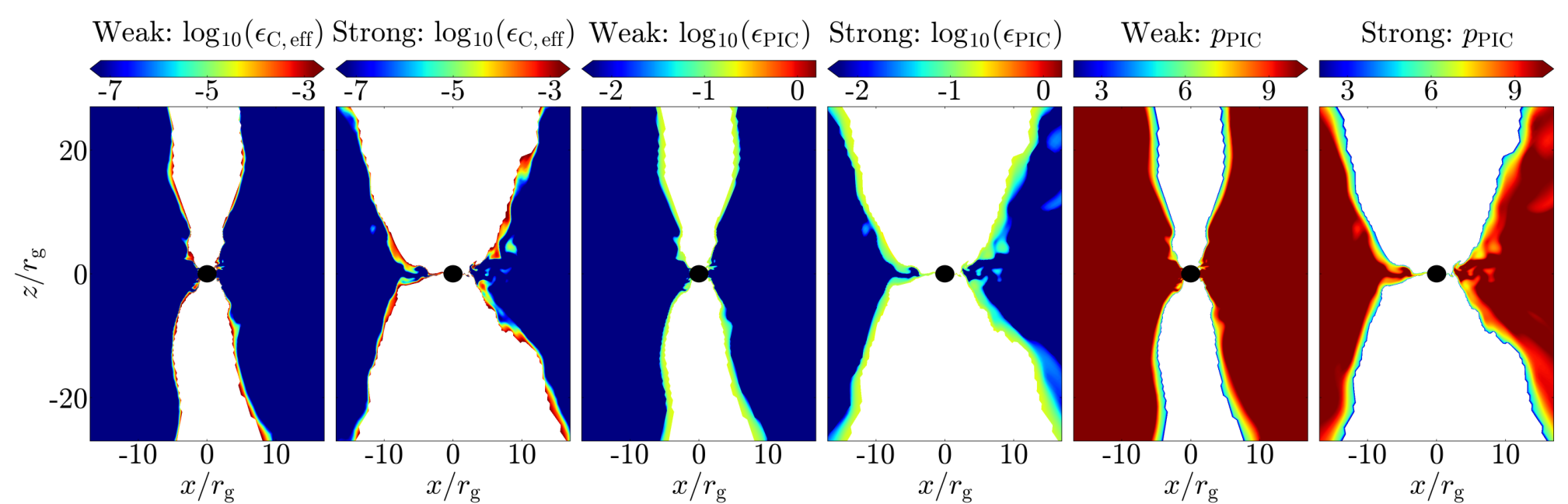
Given that the non-thermal acceleration efficiency and power-law index is sensitive to the local magnetisation and plasma-, we expect that regions of low plasma-, i.e., the jet sheath, would dominate the majority of X-ray emission. Figure 3 shows that the acceleration efficiency is indeed only significantly high in the jet sheath for the Weak model while for the Strong model, the extended jet sheath and the low plasma- near the BH both exhibit non-zero non-thermal acceleration. The individual values of the efficiency in the two non-thermal models ( and ) differ greatly due to the model definitions, i.e., one is defined as a fraction of the magnetic energy density and the other as a fraction of the electron energy density. Further, for model , we only get power-law indices less than four at the jet boundary. Thus, we see that non-thermal electrons only appear at the jet-edge in whereas there is a wider particle acceleration region in models. Further, Fig. 4 shows that the synchrotron cooling only occurs in parts of the disc and the jet sheath, where the break Lorentz factor is smaller than the power-law cutoff Lorentz factor . The spectral steepening would thus affect the X-ray emission which originates in the current sheets close to the BH.
Figure 5 shows the time evolution of our simulations, illustrating the horizon accretion rate , the horizon energy accretion rate , the horizon outflow efficiency (i.e., the ratio of the outflow power and the accretion power ), the horizon dimensionless magnetic flux (in Gaussian units) and the disc barycentric radius , defined as:
| (24) |
| (25) |
| (26) |
| (27) |
| (28) |
where , , and are the total radial energy flux, radial velocity, radial magnetic field and the metric determinant respectively (Porth et al. 2019; Chatterjee et al. 2020, standard definitions from e.g., ). The weak-field model, Weak, produces a jet with an average efficiency of while the strong-field model (Strong) jet attains an efficiency of almost . Jet efficiencies are known to occur when the magnetic pressure around the BH becomes sufficiently dominant to obstruct gas from accreting (Narayan et al. 2003; Tchekhovskoy et al. 2011, e.g.,), leading to a magnetically arrested disc (MAD) state. Indeed, as shown in Dexter et al. 2020b and Porth et al. 2021, MAD conditions lead to magnetic flux eruptions where magnetised low density bunches of field lines (i.e., flux tubes) escape from the BH’s event horizon and interact with the surrounding accretion material via shearing instabilities, heating up electrons and causing NIR flaring events (Dexter et al. 2020b).
Neither simulation develops the MAD state as they do not exhibit magnetic flux eruptions. However, Strong displays a significantly higher jet power as well as horizon magnetic flux, which considerably changes disc-jet dynamics close to the BH, especially with respect to disc turbulence. Stronger outflows lead to a higher rate of momentum transport outwards and hence causes the disc to viscously spread out as illustrated by the increasing value of over time in the case of Strong. One important question remains for MADs or even strong-field discs in the context of Sgr A∗: these types of discs always produce powerful jets that seem to be absent in Sgr A∗. From the ongoing EHT observations of Sgr A∗, we will hopefully be able to place much better constraints on the size of the source as well as the structure of the horizon-scale flow, which will prove crucial to settling the question of jets from Sgr A∗. Our goal is to understand the effect of disc or jet turbulence on variability in a quasi-stable disc whereas for MADs, the presence of magnetic eruptions distorts the inner structure of the accretion flow.

4.2 Multiwavelength spectrum of Sgr A∗: observations and GRRT modelling
We generate synchrotron spectra for each of our hybrid thermalnon-thermal models assuming the BH mass and distance of Sgr A∗ (see Table 1: GRRT parameters). From Fig. 5(a), we see that the accretion rate for each model at first increases, marking the start of accretion from the torus, and then slowly decreases and finally settles at a time for model Weak and at for model Strong. We choose a time segment spanning in excess of 60 hours for each simulation. The time duration is quite long compared to the dynamical timescales for typical flares in Sgr A∗, which are on the order of minutes to an hour. The fiducial model source inclination angle with respect to the observer is taken to be in accordance with previous Sgr A∗ models (Markoff et al. 2007; Mościbrodzka et al. 2009; Shcherbakov et al. 2012; Drappeau et al. 2013; Connors et al. 2017, e.g.,). Sgr A∗’s inclination angle is still an open question with several other works employing smaller inclinations (Dexter et al. 2010; Mościbrodzka & Falcke 2013; Chael et al. 2017; Davelaar et al. 2018; Gravity Collaboration et al. 2020b, e.g.,). Hence, we also perform the same GRRT calculations at an inclination angle of . We do not change any other parameter, such as the electron temperature distribution or the accretion rate, in order to directly compare to the fiducial inclination models. The source azimuthal angle with respect to the observer is taken to be as the BH disc-jet system is roughly axisymmetric (Chatterjee et al. 2020, this quantity only becomes important for misaligned BH discs, see). The field-of-view (FOV) for the GRRT imaging is with an image resolution of pixels.
Figure 6 shows the multiwavelength spectrum for each radiative model: the mean spectrum along with deviations, and the maximum X-ray flare spectrum. The mass accretion rate for each model is chosen to match the observed sub-mm fluxes: yr-1 for Weak and yr-1 for Strong. These accretion rates lie well within the range of yr yr-1, inferred from Faraday rotation measurements of Sgr A∗ (Bower et al. 2003; Marrone et al. 2007). The choice of and is made such that the mean spectrum roughly fits the 230 GHz flux while not overproducing the NIR emission. We note that in the case of Weak- (Fig. 6b), lower values of can be used to preferentially heat the electrons in low plasma- regions, such as the jet sheath. However, for this work, to keep the models comparable, we choose the same value of for each model, varying only and therefore the electron temperature in the disc. The change in spectral index at frequencies above Hz occurs due to synchrotron cooling, with the turnover frequency set by equating the local advective and synchrotron cooling timescales. We reiterate at this point that we do not account for inverse Compton scattering, and the Hz bump is due to non-thermal synchrotron only.
During periods of flaring, the non-thermal contribution to the NIR flux increases and affects the NIR slope in the spectra of three models (Fig. 6a,b,d), while in the case of Strong-, the thermal synchrotron emission dominates the NIR emission. None of the models are able to simultaneously reproduce the NIR GRAVITY flux and the Hornstein et al. 2007 slope, while the brightest X-ray flare spectrum of Weak- displays a similar slope, but fails to produce the required NIR flux. In the X-rays, Weak- is consistent with the quiescent X-ray flux while Weak- displays a low X-ray quiescent flux. The mean spectrum for the strong-field models overproduce the quiescent X-ray limits. Since the inner disc in Strong is highly magnetised, we see higher X-ray emission overall with model Strong- achieving the brightest flare with an X-ray luminosity exceeding the average flare luminosity. Among the models that produce X-ray luminosities above quiescence, Weak- produces the largest relative change in X-ray luminosity between the mean and brightest flare spectrum with a difference of over an order of magnitude. It is further encouraging to note that in the case of the PIC-motivated radiation models, the change in power-law index of the non-thermal distribution occurs at Hz due to synchrotron cooling and hence, the X-ray power-law index during the brightest flares is , consistent with the photon indices measured by Nowak et al. 2012 and Haggard et al. 2019. This result verifies the claim that simultaneous NIR and X-ray flares are perhaps related via a broken power-law distribution (Dodds-Eden et al. 2010; Dibi et al. 2014; Ponti et al. 2017, e.g.,), and strongly points towards a non-thermal origin for Sgr A∗ flaring. We note that the synchrotron spectra from our models do not display a clean cooling break as seen in semi-analytical models such as Dodds-Eden et al. 2010; Ponti et al. 2017. This difference occurs because our spectra are a summation of power-law emission from different regions in the flow while these papers use a single-zone emission model with a single broken-power-law component.
The inclination models show similar mean spectra to their inclination counterparts. If we compare the Weak- models (panels a and e), the NIR emission drops for lower inclination. This reduction occurs because the NIR emission originates in the toroidal gas flow in the accretion flow, which is Doppler-boosted towards us at high inclinations. This effect is less evident in the Strong models since the primary source of NIR photons is the broad jet sheath. The X-ray spectra do not change significantly when changing the inclination angle since this is optically thin synchrotron emission. We will discuss variability in the low inclination case in the next section.
4.3 Disc-averaged profiles

Figure 7 shows the disc-averaged values of the electron number density in cm-3, magnetic field strength in Gauss, and the ion and electron temperatures, and respectively, in Kelvin for both Weak and Strong simulations, when scaled to the BH mass of Sgr A∗ and the aforementioned accretion rates. The disc-averaging for a parameter is calculated in the form
| (29) |
similar to the evaluation of the barycentric radius in the previous section. As mentioned in the previous section, from Fig. 5(d), we see that the strong-field Strong disc grows larger over time and hence, becomes more diffused, leading to lower values in the disc as compared to the weak-field model Weak (Fig. 7a). Even though the Strong ion temperature is higher, the electron temperatures from the two simulations are roughly similar in the disc since the parameter for Strong is 4 times as large as for Weak. In the next section, we study the variable properties of the observed lightcurves that are the outcome of disc turbulence and magnetic reconnection in the current sheets.
5 Variability in lightcurves

In this section, we perform timing analysis of the radiative models studied in the previous section. We consider three specific wave bands and compare our results with three corresponding observational papers: 230 GHz - Dexter et al. 2014, 2.12 m - Do et al. 2019 and 2-8 keV - Neilsen et al. 2015. Figure 8 shows the lightcurves in each of the three bands at inclination , for each model (Table 1). For comparison with the observational data, we construct the fractional root-mean-square (rms) normalised power spectral density (PSD) curves for each set of lightcurves (Fig. 10) and cumulative distribution functions (CDFs) for the 2.2 m and X-ray lightcurves (Figs. 11, 12 and 13). To reduce noise at high frequencies in the PSDs, we re-bin logarithmically and average over frequency bins. In the following subsections, we look at each waveband in turn and discuss the lightcurves, PSDs and CDFs for each inclination model and then compare to the corresponding inclination case.

5.1 Sub-millimetre: 230 GHz
Figure 8(a) shows that the weak-field model 230 GHz lightcurves- Weak- and Weak- are similar to each other on average and show an increase of a factor in the flux at late times, largely following the variations in the accretion rate. For the strong-field disc cases, Strong- and Strong-, the lightcurves behave quite similarly: the 230 GHz lightcurves lie almost on top of each other. The similarity in the lightcurves suggests that the bulk of the 230 GHz emission is being produced in the same region for each GRMHD model, as is expected since the emission is thermal in nature and there is only one electron temperature distribution for each simulation model. The accretion rate is scaled such that the 230 GHz flux is the same for all models. However, as seen from the average spectrum in Fig. 6(a) vs (b), there is a noticeable addition to the terahertz flux in the case of model Weak- due to the presence of a higher percentage of thermal electrons in the jet sheath in comparison to Weak-. This difference in the terahertz flux is due to the acceleration prescription used in Weak- where magnetic energy is transferred to the non-thermal energy density. Hence, the regions closest to the BH (where the magnetic field is the strongest) is favoured as the region of electron acceleration as opposed to the jet sheath. However, for the strong-field radiative models, the radio-to-infrared spectra are almost similar. The inclination 230 GHz lightcurves in Fig. 9(a) display a higher flux as compared to the inclination models as the image becomes more extended at low inclinations.

Figure 10(a) shows the 230 GHz PSD as a function of the Fourier sampling frequency () for each model. At high frequencies, all models behave like red noise with a power-law dependence on of . The 230 GHz rms% value of all the models (Table 2) matches the accretion rate rms% as well as the observed 20-30% variation seen in the sub-mm lightcurves of Sgr A∗ (Zhao et al. 2003; Marrone et al. 2008; Dexter et al. 2014, e.g.,). For the weak-field models, the red-to-white turnover occurs at frequencies close to min-1 pointing to a characteristic variability timescale () of the order of tens of hours. For the strong-field model, the turnover appears to occur at slightly higher frequencies ( min-1), which is close to measured variability timescale of Sgr A∗ (Dexter et al. 2014, hours of Sgr A∗;). Currently, the lowest frequency bins in the averaged PSDs contain a single datapoint, and hence the standard error for each bin is equal to the power itself, which would introduce large error-bars for the best-fit value of variability timescale. Capturing the white noise regime properly is essential for accurately fitting for the variability timescale, and hence, requires a lightcurve that is at least one order of magnitude longer than that calculated in this study.
5.2 Near-infrared: m
| Mean flux & | ||||
| Model | 230 GHz | 2.12 m | 2-8 keV | |
| [Jy & %] | [mJy & %] | [ergs cm-2 s-1 & %] | ||
| Inclination: | ||||
| Weak- | , 31.58% | , 158.70% | , 143.94% | 24.5% |
| Weak- | , 34.76% | , 304.59% | , 275.63% | 24.5% |
| Strong- | , 25.33% | , 123.66% | , 33.05% | 23.8% |
| Strong- | , 24.43% | , 61.33% | , 45.04% | 23.8% |
| Inclination: | ||||
| Weak- | , 38.20% | , 144.00% | , 117.17% | 24.5% |
| Weak- | , 35.34% | , 150.42% | , 293.47% | 24.5% |
| Strong- | , 23.50% | , 126.64% | , 31.06% | 23.8% |
| Strong- | , 23.01% | , 60.96% | , 45.04% | 23.8% |

Figure 8(b), 9(b), 10(b) and 11 show the lightcurves, power spectra and the cumulative distribution functions at 2.12 m (NIR) wavelength. We see that the Weak- and Strong- NIR lightcurves display, on average, higher fluxes than that for Weak- and Strong-, repectively. The PSDs for the strong-field models are similar and display a power-law slope close to . The weak-field model PSDs are strikingly different from the strong-field cases, exhibiting flatter slopes at high Fourier frequencies. This is consistent with variability in extremely low fluxes being uncorrelated events, in the form of multiple weakly magnetised current sheets in the accretion flow. The inclination Weak model PSDs have slightly steeper slopes at high frequencies than the corresponding high inclination models.
The weak-field NIR lightcurves display high rms variability with rms% values for Weak- and for Weak- (Table 2), which stems from the rapidly fluctuating non-thermal component. These values are close to the observed NIR rms amplitude (Witzel et al. 2018, ;). This can be seen from Fig. 8(b) as the flux from both models (blue solid line for Weak- and teal dash-dotted line for Weak-) vary by a factor of 100 over the lightcurve duration. In the low inclination case, the mean NIR flux decreases for all models (see Table 2) while the rms% remains similar. One noticeable change is in the Weak- rms% that drops by a factor of 2.
One way to decrease the rms% is to account for synchrotron self-Compton (SSC) upscattering of thermal synchrotron photons as this process might contribute significantly during low flux states in the infra-red (e.g., as seen from Fig. 2 in Mościbrodzka et al. 2009, also see Eckart et al. 2004). The importance of low-level flux events in the overall flux distribution is illustrated more clearly in the CDFs, shown in Fig. 11.
The CDF () is defined as the fraction of the total number of GRRT snapshots () where the emitted flux at a given frequency exceed or equals a certain threshold flux ,
| (30) |
where are the fluxes for each GRRT time snapshot, and and for the weak-field and strong-field models, respectively. In Fig. 11, we see that the strong-field models display similar quiescent flux levels to those from Do et al. 2019, but do not show enough high flux events. The lack of high flux events can be explained via the strong-field spectra (Fig. 6 c and d) where we see that the NIR spectrum shows less variability compared to the weak-field models, and there are not enough high level flux events to skew the CDF towards a power-law. For the weak-field models, the situation is entirely different as there are too few moderate level flux events and hence, the CDF transitions to a steeper power-law at a smaller flux threshold than for the observed CDF. Here, SSC can contribute to the moderate and low flux levels and skew the CDF transition flux threshold to a higher value. Assuming this flare is due to the same processes, more efficient electron acceleration must occur to explain the high flux excursions as seen in Do et al. 2019. A log-normal power-law-tail distribution describes the weak-field model CDFs better than a log-normal distribution, consistent with the results of Dodds-Eden et al. 2010; Petersen & Gammie 2020. The slopes of the individual CDFs are also interesting to note in the context of log-normal versus power-law CDF distributions. All models except Strong- display a slope close to -2 and also have rms% exceeding 120%. The Strong- CDF, on the other hand, shows a comparatively steeper slope closer to -4, similar to the values found for lightcurves in Witzel et al. 2012; Witzel et al. 2018, as well as a relatively low rms of 60%. It could be that changes in the accretion rate drive the NIR variability in this model, and therefore, give rise to the log-normal flux distribution.
It is interesting to note that the low inclination Weak NIR CDFs do not show the power-law tail. In the case of Weak-, it could be due to a change in Doppler-boosting of the emission as the background jet sheath flow is predominantly toroidal. For the Weak- case, the mean NIR flux drops by an order of magnitude and hence the corresponding CDF changes. The Strong model CDFs remain similar to the corresponding high inclination case. This behaviour of the CDFs suggests that the log-normal component of the CDF is independent of the inclination while the power-law tail can change with inclination. Further, from the Weak NIR PSDs, it appears that there is a correlation between a shallow PSD slope at high fourier frequencies and a power-law tail in the CDF, i.e., when the PSD slope steepens, the power-law tail disappears. It follows that the varying accretion rate of the turbulent disc material naturally creates low-flux events, while individual strong reconnection events trigger the formation of fast-moving short-lived blobs of plasma that produce the high NIR flux events, in line with the GRAVITY NIR hotspot observations. Semi-analytical work with hotspot models (Broderick & Loeb 2006; Younsi & Wu 2015, e.g.,) has already shown that the lightcurve is strongly inclination-dependent. Thus, higher resolution GRMHD simulations that capture plasmoid formation would be crucial in confirming the inclination dependence of the NIR CDF.
5.3 X-rays: 2-8 keV
Figures 8(c), 9(c) and 10(c) show the 2-8 keV lightcurves given in units of erg cm-2 s-1 and the corresponding power spectra for each model, respectively. First we discuss the inclination lightcurves. From Sec. 4.2, we see that model Weak- displays a mean spectrum over the considered time duration of hours that coincides with the total quiescent X-ray emission of Sgr A∗ from Nowak et al. 2012. The lack of any variability in the quiescent spectrum over two decades of observations strongly favours the origin to be thermal bremsstrahlung emission from close to Bondi scales (Quataert 2002, e.g.,), which is supported by the resolve extension beyond Chandra’s PSF (Wang et al. 2013). The high mean emission from this model is the outcome of an increase in the accretion rate over the time segment, that also drives a steady increase in the 230 GHz flux (Fig. 8a: blue solid line). On the other hand, Weak- produces an X-ray lightcurve that is considerably dimmer, even failing to reproduce the expected quiescent non-thermal emission (Neilsen et al. 2013, of the quiescent emission). The weak-field X-ray lightcurves are less variable as compared to their NIR counterparts, with a rms amplitude of (for Weak-; Table 2) and (for Weak-). These values are within an order of magnitude of the observed rms amplitude in X-rays () for Sgr A∗. The strong-field models exhibit similar lightcurves to each other, with Strong- displaying higher flux levels than Strong- almost throughout the chosen time duration. The low rms% in the Strong models indicate that the variability in the spectra for the strong-field models is quite low, suggesting that the strongly magnetised current sheets in the inner accretion disc, (as seen from the low plasma beta in the region, Fig. 2 bottom row, middle panel), are structurally stable in time despite the turbulence in the disc. The strong-field model PSDs look similar with comparable rms%, as the origin of the emission is the same in the two radiative models: the low plasma- jet sheath. The small difference in the variability between Strong- and Strong- is more noticeable in their flux distributions, which we calculate next.
To directly compare our X-ray CDFs to those obtained from the Chandra 3 Ms Sgr A∗ 2012 X-ray Visionary Project, we closely follow the methodology given in Neilsen et al. 2015. We process our GRRT X-ray lightcurves using the same tools used to analyse observed Chandra lightcurves. To this effect, we use the Interactive Spectral Interpretation System (Houck & Denicola 2000, ISIS;) to fold our model lightcurves with High Energy Transmission Grating Spectrometer (HETGS) Chandra Sgr A∗ responses from Nowak et al. 2012. Following Sec. 4.1 in Nowak et al. 2012, we include interstellar absorption with the model TBnew (Wilms et al. 2000) with Verner et al. 1996 cross-sections, assuming the hydrogen column density cm-2. We then calculate the predicted 2-8 keV count rates. We derive the zeroth order count rates as well as the first order count rates for both HETG grating sets, the medium-energy gratings (MEG) and the high-energy gratings (HEG). We reduce the simulated zeroth order count rates for photon pileup assuming the same scaling as in Neilsen et al. 2015 since this effect may be as strong as 10-15% for the highest count rates. We then combine the zeroth and first order count rates to calculate the final intrinsic lightcurve (i.e., this does not include the quiescent emission). For the CDF calculation, we assume a quiescent background X-ray count rate of 5.24 counts/ks to represent the bremsstrahlung contribution from larger scales, adding Poisson noise and interpolating the processed lightcurve onto 300 s bins as done in Neilsen et al. 2015.
Figures 12 and 13 show the obtained CDFs and the 2D probability contour plots for the weak-field and strong-field models. We represent each radiative model CDF (black lines in the figures) as a combination of a Poisson process (blue dashed) with rate Qpl to characterise the low flux level quiescent emission, and a power-law tail (red dashed) with index for the flare emission. Following Neilsen et al. 2015, we then run Markov Chain Monte Carlo simulations (grey lines) to find maximum likelihood fits for Qpl and and compare to the best fit values obtained from Chandra observations, given in Neilsen et al. 2015: Q counts/ks and .
Weak- exhibits a higher Poisson rate Q counts/ks and smaller power-law index of as compared to and (Fig. 12). Hence, Weak- slightly overproduces the quiescent flux-level and reasonably describes the flux distribution for flaring events. Due to the limited duration of our lightcurves, decomposing the CDF into the quiescent Poissonian and power-law tail from the quiescent yields errors larger than those from the Chandra XVP data. For Weak-, the background quiescent flux completely dominates the flux distribution, as is expected from the lightcurve. Strong- exceeds the Sgr A∗ Poisson rate Qpl,bf and displays no traces of a power-law flux distribution at high flux levels. Strong- exhibits a Poisson rate that is larger than Qpl,bf by a factor of , with a power-law index that is steeper than the measured index , indicating that there is an overabundance of high-level fluxes, and few flaring excursions beyond the calculated quiescent level (e.g., the maximum X-ray flare spectrum in Fig. 6d). It is possible to reduce the acceleration efficiency for models Weak- and Strong- in order to achieve the correct Qpl value. However models Weak- and Strong- are dependent entirely on plasma- and magnetisation, and do not have any free parameters to adjust the X-ray output.
Overall, only Weak- provides a reasonable description of the X-ray flux distribution in Sgr A∗. As mentioned in Sec. 4.2, the X-ray emission in our models is optically thin synchrotron and, thus, inclination-independent. Consequently, the PSDs and the CDFs do not change significantly with inclination (see Fig. 13). Combining this information with the absence of the power-law tail in some of the NIR CDFs, it is possible that X-ray-emitting blobs that form near the BH might eventually travel along the jet sheath with relativistic speeds and begin to emit in the NIR band. This is one way that Doppler-boosting might play a pivotal role in determining the CDF shape.
6 Discussion and conclusions
| Summary Table | ||||||
|---|---|---|---|---|---|---|
| Model | NIR | X-ray | ||||
| quiescent flux | CDF slope | rms% | Qpl | CDF slope | rms% | |
| Inclination: | ||||||
| Weak- | Pass | Pass | Pass | Pass | Pass | |
| Weak- | Pass | Pass | Pass | |||
| Strong- | Pass | Pass | Pass | |||
| Strong- | Pass | Pass | ||||
| Inclination: | ||||||
| Weak- | Pass | Pass | Pass | Pass | Pass | |
| Weak- | Pass | Pass | Pass | Pass | ||
| Strong- | Pass | Pass | Pass | |||
| Strong- | Pass | Pass |
The flaring activity in Sgr A∗ observed in the NIR/X-ray bands provides important clues about the physics of particle energisation and acceleration in the inner few gravitational radii around a SMBH. Current sheets occur naturally in the turbulent, magnetised regions of the disc and will inevitably lead to magnetic reconnection of field lines. Magnetic reconnection results in thermal heating of both electrons and ions, and accelerates a fraction of the electron population to a non-thermal power-law distribution. The nearest SMBH, Sgr A∗, is monitored well enough to extract statistical information about the nature of flaring events, e.g., the observed flux distributions and power spectra in the sub-mm, NIR and X-ray wavebands. Here, we take advantage of these measured quantities to test whether the combination of synchrotron emission from non-thermal electrons and disc/jet turbulence can explain the general properties of the flaring events.
GRMHD simulations are able to capture MHD turbulence in addition to accurately describing the effects of general relativity in the extreme gravity of black holes (Sec. 2). Ideal GRMHD, by definition, does not include dissipative processes such as particle acceleration and the effects of radiation, and hence, to directly compare our simulations with observations of Sgr A∗, we rely on an additional layer of modelling for the electron properties, together with GRRT radiative transfer as a post-processing step (Sec. 3). Using this procedure, we calculate the multiwavelength spectra of our GRMHDGRRT radiative models (Sec. 4.2), scaling the black hole mass and distance to that of Sgr A∗ with an accretion rate of a few yr-1 that provides a reasonable match to the observed sub-mm flux at two different inclination angles ( and ). We only consider synchrotron emission, both from thermal and non-thermal electron populations. Further, to study the variability of our simulation lightcurves, we derive the power spectra and cumulative distribution functions in 3 wavelengths: 230 GHz (sub-mm), m (NIR) and 2-8 keV (X-rays) and compare with their observed counterparts (Dexter et al. 2014; Neilsen et al. 2015; Witzel et al. 2018, (Sec. 5)).
Table 3 shows the variability results from this work in a concise way. We find that one of our models, Weak-, describes the data reasonably well: (1) the mean spectrum is within observational quiescent limits, (2) the brightest flare X-ray luminosity matches the average X-ray flare spectrum from Neilsen et al. 2015, and (3) the X-ray lightcurve is quite variable and the calculated CDF resembles Sgr A∗’s X-ray CDF. However, Weak-’s brightest flare X-ray luminosity is 25 times smaller than the Haggard et al. 2019 Chandra flare. Further, the X-ray lightcurve does not look similar to observed lightcurves, where flares usually span over longer timescales as compared to the flares obtained from our models. This could be a result of using the “fast-light” approximation in our GRRT method, which could become invalid in the vicinity of the black hole, where the photon travel time becomes comparable to the timescale at which the plasma distribution changes (Ball et al. 2021, e.g.,). The NIR CDF follows a log-normal power-law-like distribution as expected from observations, but has a lower quiescent flux level than that measured for Sgr A∗. This model has a relatively weak magnetic flux content in the disc, otherwise known as the “standard and normal evolution” (SANE) model, as opposed to near-magnetically arrested strong-field models. The strong-field models, on average, overproduce the quiescent X-ray limits and exhibit a lower level of variability in the X-ray lightcurves as compared to Sgr A∗. Thus we favour disc turbulence in SANE models as a reasonable mechanism for explaining Sgr A∗’s average flare properties.
None of our models can account for the extremely bright NIR flaring reported in Do et al. 2019, though we do achieve moderately high fluxes. There are three possible explanations as to why. It is probable that one needs a pronounced increase in the accretion rate to explain these flares, as suggested by Do et al. 2019. If we consider the strong-field model Strong-, changes in the accretion primarily drive fluctuating flux levels as seen from the variation in the spectrum (grey region in Fig. 6d) and the brightest X-ray flare spectrum, where the sub-mm and NIR flux both increase by a factor of with respect to the mean spectrum. However, turbulence-driven variability is not enough to explain isolated high luminosity events, and we require GRMHD simulations with enough resolution to capture plasmoid formation. Indeed, as Gutiérrez et al. 2020 suggests, a sufficiently strong non-thermal event may be able to explain the Do et al. 2019 observations. However, the resemblance between our calculated CDFs and the measured CDF from Do et al. 2019 suggests that processes that frequently occur in the disc and the jet sheath, such as magnetic reconnection in current sheets and variations in the accretion rate, drive most moderate level NIR flux events (also see Petersen & Gammie 2020). A third possibility is the uncertainty in our assumed electron temperature model, i.e., the turbulent-heating motivated electron temperature model from Howes 2010; Mościbrodzka et al. 2016. There are alternate electron temperature prescriptions (Mościbrodzka et al. 2009; Dexter et al. 2010; Anantua et al. 2020, e.g.,) as well as electron heating models that consider magnetic reconnection and plasma turbulence (Rowan et al. 2017; Werner et al. 2018; Kawazura et al. 2019; Zhdankin et al. 2019). Indeed, Dexter et al. 2020a shows that the radio-to-NIR spectrum depends significantly on whether the electrons get heated by turbulence (Howes 2010) or reconnection (Werner et al. 2018). Similar to our weak-field models, Dexter et al. 2020a finds high rms% in the NIR, though the NIR emission originates from only thermal electrons. Interestingly, they also find that heating due to reconnection offers higher variability. Finally, they favour a magnetically arrested disc (MAD) model with reconnection-based electron heating, as weak-field models fail to produce the observed linear polarisation fraction. MAD disc models offer an interesting alternate source of variability: magnetic eruptions (Tchekhovskoy et al. 2011, e.g.,) that lead to significant changes in the disc and jet morphology, and contribute to the NIR variability (Dexter et al. 2020b; Porth et al. 2021). Further, recent simulations of the large scale evolution of the accretion flow starting from the Bondi sphere up to the event horizon by Ressler et al. 2020 also favour a large magnetic flux near the black hole of Sgr A∗. However, MAD models are difficult to motivate due to the apparent absence of a strong jet in Sgr A∗. In this work, our goal is to examine variability due to turbulence-driven reconnection in relatively-stable discs, and hence, we leave an exploration of MADs for future work.
Other alternate sources of variability include radiative cooling (Fragile & Meier 2009; Dibi et al. 2012; Yoon et al. 2020, e.g.,), jet-wind boundary instabilities (McKinney 2006; Bromberg & Tchekhovskoy 2016; Chatterjee et al. 2019, e.g.,) and misalignment between the black hole spin vector and the disc angular momentum vector (Dexter & Fragile 2013; White et al. 2020; Chatterjee et al. 2020). It is possible that our conclusions may change with the addition of radiative cooling within the GRMHD simulation. Synchrotron and inverse Compton cooling removes internal energy from the gas and changes the dynamics of the turbulence, thereby altering the disc density and temperature profile, even for accretion rates similar to Sgr A∗ (Yoon et al. 2020). Hence, if the electron temperature and the acceleration efficiency in the disc current sheets become small enough to satisfy the quiescent NIR and X-ray limits, strong-field models might become a viable option. Indeed, in strong-field models, collisions between the jet and the disc-wind/environment can lead to pinch and kink mode instabilities that efficiently dissipate magnetic energy as heat and/or accelerate particles, as well as lead to enhanced gas entrainment into the jet (Chatterjee et al. 2019, e.g.,). Finally, misalignment between the black hole spin and the disc may lead to possible turbulent heating events as well as enhanced jet-wind collisions (Dexter & Fragile 2013; White et al. 2020; Chatterjee et al. 2020). In order to accurately track particle acceleration due to the reconnection events around black holes, we would require general relativistic PIC simulations (Crinquand et al. 2020, e.g.,). Alternatively, in GRMHD, one can use test particles (Ripperda et al. 2019; Bacchini et al. 2019, e.g.,) or evolve the electron distribution function (Chael et al. 2017; Petersen & Gammie 2020, e.g.,). All of these methods improve upon the postprocessing method we use in this work. Advanced models of electron thermodynamics and non-conventional disc geometries will no doubt contribute not only to the overall variability of Sgr A∗ across its entire multiwavelength emission, but also inform our interpretation of the upcoming 230 GHz Event Horizon Telescope image of Sgr A∗. This work is meant to be a first study of non-thermal activity in high resolution 3D GRMHD simulations and further exploration of GRMHD simulations with alternate black hole spins, disc/jet morphologies and orientations, imaged at a variety of inclination angles are required to constrain the possible parameter space of Sgr A∗ models.
In conclusion, this work presents the first study comparing NIR/X-ray statistics produced from the best available dynamical models of Sgr A∗ to observations, focusing on variability due to turbulence-driven reconnection. We perform GRRT radiative transfer calculations on two 3D GRMHD models of accreting black holes, one with a weakly magnetised disc and the other a strong-field case, using two different realisations of a hybrid thermalnon-thermal electron energy distribution, and generate 230 GHz, m and 2-8 keV lightcurves over a period of time exceeding 60 hours. Table 3 shows the time-averaged flux as well as the variability results from our study. A summary of our results is as follows:
- 1.
Weakly magnetised discs exhibit high levels of variability in the NIR and the X-rays. Our simulations show that a broken power-law spectrum produces NIR and X-ray CDFs with a slope , and can be used to explain CDFs of simultaneous NIR/X-ray flares.
- 2.
Non-thermal synchrotron emission due to disc turbulence in weak-field models explains the average X-ray flare spectrum and flux distribution of Sgr A∗ reasonably well (see Table 3).
- 3.
Strongly magnetised discs exhibit low variability as highly magnetised plasma is more abundantly found in the disc and jet sheath. Synchrotron emission from both thermal and non-thermal electron populations contribute to the NIR flux while X-rays originate from non-thermal electrons.
- 4.
Overall, inclination does not seem to affect NIR and X-ray variability. However, it is possible that Doppler boosting may affect any NIR emission originating in the jet sheath. X-ray emitting plasmoids can travel along the jet sheath, cool and begin to emit in the NIR waveband.
- 5.
Disc turbulence alone cannot explain the highly luminous Sgr A∗ NIR and X-ray flares from Do et al. 2019 and Haggard et al. 2019 respectively.
From our study, it is apparent that we require simulations that are able to resolve the tiny length-scales of plasmoids in order to explain the bright flares seen in Do et al. 2019 and Haggard et al. 2019. We have seen 2D versions of such simulations only recently (Nathanail et al. 2020; Ripperda et al. 2020). These simulations suggest that we require grid resolutions in excess of 2000 cells across the disc height to trigger the plasmoid instability, indicating that 3D simulations would push us to the brink of computational limitations. Indeed, Porth et al. 2019 showed that variability in the mass accretion rate of weak-field discs decreases with increasing grid resolution, which can have a direct effect on the sub-millimetre variability. It is, however, encouraging to note that our results indicate that one can rely on resolutions similar to this paper to study MHD turbulence-driven variability as a source of moderate level flares in Sgr A∗.
Acknowledgements
We thank the anonymous referee for the detailed suggestions that greatly improved the paper. This research was enabled by support provided by grant no. NSF PHY-1125915 along with a INCITE program award PHY129, using resources from the Oak Ridge Leadership Computing Facility, Summit, which is a DOE office of Science User Facility supported under contract DE-AC05- 00OR22725, and Calcul Quebec (http://www.calculquebec.ca) and Compute Canada (http://www.computecanada.ca). The authors acknowledge the Texas Advanced Computing Center (TACC) at The University of Texas at Austin for providing HPC and visualisation resources (allocation AST20011) that have contributed to the research results reported within this paper (http://www.tacc.utexas.edu). KC, SM and DY are supported by the Netherlands Organisation for Scientific Research (NWO) VICI grant (no. 639.043.513). K.C. is also supported by a Black Hole Initiative Fellowship at Harvard University, which is funded by grants from the Gordon and Betty Moore Foundation, John Templeton Foundation and the Black Hole PIRE program (NSF grant OISE-1743747). The opinions expressed in this publication are those of the authors and do not necessarily reflect the views of the Moore or Templeton Foundations. ZY is supported by a UKRI Stephen Hawking Fellowship and acknowledges support from a Leverhulme Trust Early Career Fellowship, MvdK is supported by the NWO Spinoza Prize, AT by Northwestern University and by National Science Foundation grants AST-1815304, AST-1911080, and AI by a Royal Society University Research Fellowship. DH acknowledges support from the Natural Sciences and Engineering Research Council of Canada (NSERC) Discovery Grant, the Canada Research Chairs program, and the Canadian Institute for Advanced Research (CIFAR). This research has made use of NASA’s Astrophysics Data System.
Data Availability
Data used to plot the images in this work is available at http://doi.org/10.5281/zenodo.5044837.
References
- An et al. (2005) An T., Goss W. M., Zhao J.-H., Hong X. Y., Roy S., Rao A. P., Shen Z. Q., 2005, ApJ, 634, L49
- Anantua et al. (2020) Anantua R., Ressler S., Quataert E., 2020, MNRAS, 493, 1404
- Bacchini et al. (2019) Bacchini F., Ripperda B., Porth O., Sironi L., 2019, ApJS, 240, 40
- Baganoff et al. (2001) Baganoff F. K., et al., 2001, Nature, 413, 45
- Baganoff et al. (2003) Baganoff F. K., et al., 2003, ApJ, 591, 891
- Balbus & Hawley (1991) Balbus S. A., Hawley J. F., 1991, ApJ, 376, 214
- Ball et al. (2016) Ball D., Özel F., Psaltis D., Chan C.-k., 2016, ApJ, 826, 77
- Ball et al. (2018) Ball D., Sironi L., Özel F., 2018, ApJ, 862, 80
- Ball et al. (2021) Ball D., Özel F., Christian P., Chan C.-K., Psaltis D., 2021, ApJ, 917, 8
- Barrière et al. (2014) Barrière N. M., et al., 2014, ApJ, 786, 46
- Boehle et al. (2016) Boehle A., et al., 2016, ApJ, 830, 17
- Bower et al. (2003) Bower G. C., Wright M. C. H., Falcke H., Backer D. C., 2003, ApJ, 588, 331
- Bower et al. (2015) Bower G. C., et al., 2015, ApJ, 802, 69
- Bower et al. (2019) Bower G. C., et al., 2019, ApJ, 881, L2
- Boyce et al. (2019) Boyce H., et al., 2019, ApJ, 871, 161
- Brinkerink et al. (2015) Brinkerink C. D., et al., 2015, A&A, 576, A41
- Broderick & Loeb (2006) Broderick A. E., Loeb A., 2006, MNRAS, 367, 905
- Broderick & McKinney (2010) Broderick A. E., McKinney J. C., 2010, ApJ, 725, 750
- Bromberg & Tchekhovskoy (2016) Bromberg O., Tchekhovskoy A., 2016, MNRAS, 456, 1739
- Chael et al. (2017) Chael A., Narayan R., Sä dowski A., 2017, MNRAS, 470, 2367
- Chael et al. (2018) Chael A., Rowan M., Narayan R., Johnson M., Sironi L., 2018, MNRAS, 478, 5209
- Chan et al. (2015) Chan C.-k., Psaltis D., Özel F., Medeiros L., Marrone D., Sadowski A., Narayan R., 2015, ApJ, 812, 103
- Chatterjee et al. (2019) Chatterjee K., Liska M., Tchekhovskoy A., Markoff S. B., 2019, MNRAS, 490, 2200
- Chatterjee et al. (2020) Chatterjee K., et al., 2020, MNRAS, 499, 362
- Connors et al. (2017) Connors R. M. T., et al., 2017, MNRAS, 466, 4121
- Crinquand et al. (2020) Crinquand B., Cerutti B., Philippov A., Parfrey K., Dubus G., 2020, Phys. Rev. Lett., 124, 145101
- Davelaar et al. (2018) Davelaar J., Mościbrodzka M., Bronzwaer T., Falcke H., 2018, A&A, 612, A34
- Davelaar et al. (2019) Davelaar J., et al., 2019, A&A, 632, A2
- Degenaar et al. (2015) Degenaar N., Wijnands R., Miller J. M., Reynolds M. T., Kennea J., Gehrels N., 2015, Journal of High Energy Astrophysics, 7, 137
- Dexter & Fragile (2013) Dexter J., Fragile P. C., 2013, MNRAS, 432, 2252
- Dexter et al. (2009) Dexter J., Agol E., Fragile P. C., 2009, ApJ, 703, L142
- Dexter et al. (2010) Dexter J., Agol E., Fragile P. C., McKinney J. C., 2010, ApJ, 717, 1092
- Dexter et al. (2012) Dexter J., McKinney J. C., Agol E., 2012, MNRAS, 421, 1517
- Dexter et al. (2014) Dexter J., Kelly B., Bower G. C., Marrone D. P., Stone J., Plambeck R., 2014, MNRAS, 442, 2797
- Dexter et al. (2020a) Dexter J., et al., 2020a, MNRAS, 494, 4168
- Dexter et al. (2020b) Dexter J., et al., 2020b, MNRAS, 497, 4999
- Dibi et al. (2012) Dibi S., Drappeau S., Fragile P. C., Markoff S., Dexter J., 2012, MNRAS, 426, 1928
- Dibi et al. (2014) Dibi S., Markoff S., Belmont R., Malzac J., Barrière N. M., Tomsick J. A., 2014, MNRAS, 441, 1005
- Dibi et al. (2016) Dibi S., Markoff S., Belmont R., Malzac J., Neilsen J., Witzel G., 2016, MNRAS, 461, 552
- Do et al. (2019) Do T., et al., 2019, ApJ, 882, L27
- Dodds-Eden et al. (2009) Dodds-Eden K., et al., 2009, ApJ, 698, 676
- Dodds-Eden et al. (2010) Dodds-Eden K., Sharma P., Quataert E., Genzel R., Gillessen S., Eisenhauer F., Porquet D., 2010, ApJ, 725, 450
- Doeleman et al. (2008) Doeleman S. S., et al., 2008, Nature, 455, 78
- Drappeau et al. (2013) Drappeau S., Dibi S., Dexter J., Markoff S., Fragile P. C., 2013, MNRAS, 431, 2872
- EHTC et al. (2019a) EHTC et al., 2019a, ApJ, 875, L1
- EHTC et al. (2019b) EHTC et al., 2019b, ApJ, 875, L5
- Eckart et al. (2004) Eckart A., et al., 2004, A&A, 427, 1
- Falcke et al. (1998) Falcke H., Goss W. M., Matsuo H., Teuben P., Zhao J.-H., Zylka R., 1998, ApJ, 499, 731
- Falcke et al. (2000) Falcke H., Melia F., Agol E., 2000, ApJ, 528, L13
- Fishbone & Moncrief (1976) Fishbone L. G., Moncrief V., 1976, ApJ, 207, 962
- Fouka & Ouichaoui (2009) Fouka M., Ouichaoui S., 2009, ApJ, 707, 278
- Fouka & Ouichaoui (2014) Fouka M., Ouichaoui S., 2014, MNRAS, 442, 979
- Fragile & Meier (2009) Fragile P. C., Meier D. L., 2009, ApJ, 693, 771
- Gammie & Popham (1998) Gammie C. F., Popham R., 1998, ApJ, 498, 313
- Genzel et al. (2010) Genzel R., Eisenhauer F., Gillessen S., 2010, Reviews of Modern Physics, 82, 3121
- Ghez et al. (2005) Ghez A. M., Salim S., Hornstein S. D., Tanner A., Lu J. R., Morris M., Becklin E. E., Duchêne G., 2005, ApJ, 620, 744
- Ghez et al. (2008) Ghez A. M., et al., 2008, ApJ, 689, 1044
- Gillessen et al. (2017) Gillessen S., et al., 2017, ApJ, 837, 30
- Gold et al. (2020) Gold R., Broderick A. E., et al., 2020, ApJ, 897, 148
- Gravity Collaboration et al. (2018a) Gravity Collaboration et al., 2018a, A&A, 615, L15
- Gravity Collaboration et al. (2018b) Gravity Collaboration et al., 2018b, A&A, 618, L10
- Gravity Collaboration et al. (2020a) Gravity Collaboration et al., 2020a, arXiv e-prints, p. arXiv:2004.07185
- Gravity Collaboration et al. (2020b) Gravity Collaboration et al., 2020b, A&A, 635, A143
- Guo et al. (2014) Guo F., Li H., Daughton W., Liu Y.-H., 2014, Phys. Rev. Lett., 113, 155005
- Gutiérrez et al. (2020) Gutiérrez E. M., Nemmen R., Cafardo F., 2020, ApJ, 891, L36
- Haggard et al. (2019) Haggard D., et al., 2019, ApJ, 886, 96
- Hakobyan et al. (2019) Hakobyan H., Philippov A., Spitkovsky A., 2019, ApJ, 877, 53
- Hawley et al. (2011) Hawley J. F., Guan X., Krolik J. H., 2011, ApJ, 738, 84
- Hornstein et al. (2007) Hornstein S. D., Matthews K., Ghez A. M., Lu J. R., Morris M., Becklin E. E., Rafelski M., Baganoff F. K., 2007, ApJ, 667, 900
- Houck & Denicola (2000) Houck J. C., Denicola L. A., 2000, in Manset N., Veillet C., Crabtree D., eds, Astronomical Society of the Pacific Conference Series Vol. 216, Astronomical Data Analysis Software and Systems IX. p. 591
- Howes (2010) Howes G. G., 2010, MNRAS, 409, L104
- Issaoun et al. (2019) Issaoun S., Johnson M. D., Blackburn L., et al., 2019, ApJ, 871, 30
- Kawazura et al. (2019) Kawazura Y., Barnes M., Schekochihin A. A., 2019, Proceedings of the National Academy of Science, 116, 771
- Leung et al. (2011) Leung P. K., Gammie C. F., Noble S. C., 2011, ApJ, 737, 21
- Li et al. (2015) Li Y.-P., et al., 2015, ApJ, 810, 19
- Liska et al. (2018) Liska M., Hesp C., Tchekhovskoy A., Ingram A., van der Klis M., Markoff S., 2018, MNRAS, 474, L81
- Liska et al. (2019) Liska M., et al., 2019, arXiv e-prints, p. arXiv:1912.10192
- Liu & Melia (2001) Liu S., Melia F., 2001, ApJ, 561, L77
- Lu et al. (2011) Lu R. S., Krichbaum T. P., Zensus J. A., 2011, MNRAS, 418, 2260
- Mao et al. (2017) Mao S. A., Dexter J., Quataert E., 2017, MNRAS, 466, 4307
- Markoff (2005) Markoff S., 2005, ApJ, 618, L103
- Markoff et al. (2001) Markoff S., Falcke H., Yuan F., Biermann P. L., 2001, A&A, 379, L13
- Markoff et al. (2007) Markoff S., Bower G. C., Falcke H., 2007, MNRAS, 379, 1519
- Marrone et al. (2007) Marrone D. P., Moran J. M., Zhao J.-H., Rao R., 2007, ApJ, 654, L57
- Marrone et al. (2008) Marrone D. P., et al., 2008, ApJ, 682, 373
- Matsumoto et al. (2020) Matsumoto T., Chan C.-H., Piran T., 2020, MNRAS, 497, 2385
- McKinney (2006) McKinney J. C., 2006, MNRAS, 368, 1561
- Melia & Falcke (2001) Melia F., Falcke H., 2001, ARA&A, 39, 309
- Mizuno et al. (2021) Mizuno Y., Fromm C. M., Younsi Z., Porth O., Olivares H., Rezzolla L., 2021, MNRAS,
- Mościbrodzka & Falcke (2013) Mościbrodzka M., Falcke H., 2013, A&A, 559, L3
- Mościbrodzka et al. (2009) Mościbrodzka M., Gammie C. F., Dolence J. C., Shiokawa H., Leung P. K., 2009, ApJ, 706, 497
- Mościbrodzka et al. (2016) Mościbrodzka M., Falcke H., Shiokawa H., 2016, A&A, 586, A38
- Narayan et al. (2003) Narayan R., Igumenshchev I. V., Abramowicz M. A., 2003, PASJ, 55, L69
- Narayan et al. (2012) Narayan R., SÄ dowski A., Penna R. F., Kulkarni A. K., 2012, MNRAS, 426, 3241
- Nathanail et al. (2020) Nathanail A., Fromm C. M., Porth O., Olivares H., Younsi Z., Mizuno Y., Rezzolla L., 2020, MNRAS, 495, 1549
- Neilsen et al. (2013) Neilsen J., et al., 2013, ApJ, 774, 42
- Neilsen et al. (2015) Neilsen J., et al., 2015, ApJ, 799, 199
- Nord et al. (2004) Nord M. E., Lazio T. J. W., Kassim N. E., Hyman S. D., LaRosa T. N., Brogan C. L., Duric N., 2004, AJ, 128, 1646
- Nowak et al. (2012) Nowak M. A., et al., 2012, ApJ, 759, 95
- Özel et al. (2000) Özel F., Psaltis D., Narayan R., 2000, ApJ, 541, 234
- Petersen & Gammie (2020) Petersen E., Gammie C., 2020, MNRAS, 494, 5923
- Ponti et al. (2017) Ponti G., et al., 2017, MNRAS, 468, 2447
- Porth et al. (2019) Porth O., et al., 2019, ApJS, 243, 26
- Porth et al. (2021) Porth O., Mizuno Y., Younsi Z., Fromm C. M., 2021, MNRAS, 502, 2023
- Quataert (2002) Quataert E., 2002, ApJ, 575, 855
- Quataert & Narayan (1999) Quataert E., Narayan R., 1999, ApJ, 520, 298
- Reid et al. (2019) Reid M. J., et al., 2019, ApJ, 885, 131
- Ressler et al. (2015) Ressler S. M., Tchekhovskoy A., Quataert E., Chandra M., Gammie C. F., 2015, MNRAS, 454, 1848
- Ressler et al. (2017) Ressler S. M., Tchekhovskoy A., Quataert E., Gammie C. F., 2017, MNRAS, 467, 3604
- Ressler et al. (2020) Ressler S. M., White C. J., Quataert E., Stone J. M., 2020, ApJ, 896, L6
- Ripperda et al. (2019) Ripperda B., Porth O., Sironi L., Keppens R., 2019, MNRAS, 485, 299
- Ripperda et al. (2020) Ripperda B., Bacchini F., Philippov A. A., 2020, ApJ, 900, 100
- Rowan et al. (2017) Rowan M. E., Sironi L., Narayan R., 2017, ApJ, 850, 29
- Roy & Pramesh Rao (2004) Roy S., Pramesh Rao A., 2004, MNRAS, 349, L25
- Ryan et al. (2017) Ryan B. R., Ressler S. M., Dolence J. C., Tchekhovskoy A., Gammie C., Quataert E., 2017, ApJ, 844, L24
- Rybicki & Lightman (1986) Rybicki G. B., Lightman A. P., 1986, Radiative Processes in Astrophysics
- Schödel et al. (2011) Schödel R., Morris M. R., Muzic K., Alberdi A., Meyer L., Eckart A., Gezari D. Y., 2011, A&A, 532, A83
- Serabyn et al. (1997) Serabyn E., Carlstrom J., Lay O., Lis D. C., Hunter T. R., Lacy J. H., Hills R. E., 1997, ApJ, 490, L77
- Shcherbakov et al. (2012) Shcherbakov R. V., Penna R. F., McKinney J. C., 2012, ApJ, 755, 133
- Sironi & Spitkovsky (2014) Sironi L., Spitkovsky A., 2014, ApJ, 783, L21
- Sironi et al. (2015) Sironi L., Petropoulou M., Giannios D., 2015, MNRAS, 450, 183
- Tchekhovskoy et al. (2011) Tchekhovskoy A., Narayan R., McKinney J. C., 2011, MNRAS, 418, L79
- Verner et al. (1996) Verner D. A., Ferland G. J., Korista K. T., Yakovlev D. G., 1996, ApJ, 465, 487
- Wang et al. (2013) Wang Q. D., et al., 2013, Science, 341, 981
- Werner et al. (2018) Werner G. R., Uzdensky D. A., Begelman M. C., Cerutti B., Nalewajko K., 2018, MNRAS, 473, 4840
- White et al. (2020) White C. J., Dexter J., Blaes O., Quataert E., 2020, ApJ, 894, 14
- Wilms et al. (2000) Wilms J., Allen A., McCray R., 2000, ApJ, 542, 914
- Witzel et al. (2012) Witzel G., et al., 2012, ApJS, 203, 18
- Witzel et al. (2018) Witzel G., et al., 2018, ApJ, 863, 15
- Xiao (2006) Xiao F., 2006, Plasma Physics and Controlled Fusion, 48, 203
- Yoon et al. (2020) Yoon D., Chatterjee K., Markoff S. B., van Eijnatten D., Younsi Z., Liska M., Tchekhovskoy A., 2020, MNRAS, 499, 3178
- Younsi & Wu (2015) Younsi Z., Wu K., 2015, MNRAS, 454, 3283
- Younsi et al. (2012) Younsi Z., Wu K., Fuerst S. V., 2012, A&A, 545, A13
- Younsi et al. (2016) Younsi Z., Zhidenko A., Rezzolla L., Konoplya R., Mizuno Y., 2016, Phys. Rev. D, 94, 084025
- Younsi et al. (2020) Younsi Z., Porth O., Mizuno Y., Fromm C. M., Olivares H., 2020, in Asada K., de Gouveia Dal Pino E., Giroletti M., Nagai H., Nemmen R., eds, IAU Symposium Vol. 342, IAU Symposium. pp 9–12 (arXiv:1907.09196), doi:10.1017/S1743921318007263
- Yuan & Narayan (2014) Yuan F., Narayan R., 2014, ARA&A, 52, 529
- Yuan et al. (2002) Yuan F., Markoff S., Falcke H., 2002, A&A, 383, 854
- Yuan et al. (2003) Yuan F., Quataert E., Narayan R., 2003, ApJ, 598, 301
- Zhang et al. (2017) Zhang S., et al., 2017, ApJ, 843, 96
- Zhao et al. (2001) Zhao J.-H., Bower G. C., Goss W. M., 2001, ApJ, 547, L29
- Zhao et al. (2003) Zhao J.-H., Young K. H., Herrnstein R. M., Ho P. T. P., Tsutsumi T., Lo K. Y., Goss W. M., Bower G. C., 2003, ApJ, 586, L29
- Zhdankin et al. (2019) Zhdankin V., Uzdensky D. A., Werner G. R., Begelman M. C., 2019, Phys. Rev. Lett., 122, 055101
- Zylka et al. (1995) Zylka R., Mezger P. G., Ward-Thompson D., Duschl W. J., Lesch H., 1995, A&A, 297, 83
Appendix A Non-thermal synchrotron fitting


In this section, we give a description of our synchrotron emissivity and absorption coefficient from a power-law distribution of electrons with power-law index . We take the expressions from Fouka & Ouichaoui 2014. The instantaneous integrated synchrotron spectral power for a pure power-law particle distribution with isotropic pitch angle distribution (Rybicki & Lightman 1986),
| (31) |
where , and are the Larmor gyration frequency, the synchrotron characteristic frequency, and the normalisation constant respectively. The minimum and maximum limits for the electron Lorentz factor in the power-law distribution are and . The synchrotron function is,
| (32) |
The emissivity and intensity is given by,
| (33) |
where and are the absorption coefficient and the photon pathlength respectively. Note that the optical depth is given by . Fouka & Ouichaoui 2009; Fouka & Ouichaoui 2014 parameterises the spectral power as , in terms of a dimensionless frequency with , the Lorentz factor ratio , and a normalisation coefficient,
| (34) |
The parametric function is given as,
| (35) |
where and . Here, the Fouka & Ouichaoui 2014 fitting formula for is given by,
applicable for . Here, and , as functions of the Gamma function, are,
The coefficients , , and in terms of are
Next, we come to the absorption coefficient, for , where the parametric function and the normalisation coefficient are given as,
| (36) | ||||
| (37) |
For the cooling case, i.e., the broken power-law electron distribution function, the power-law changes to at the cooling cutoff, , where is calculated by equating the local advection timescale to the synchrotron cooling timescale for electrons (see Eqn. (14)). Therefore, the distribution function becomes
| (38) |
Accordingly, the synchrotron spectral power can be split into two parts,
| (39) |
where,
| (40) |
The spectral power can be further simplified as , where and the parametric function is,
| (41) |
The corresponding extension of the absorption coefficient becomes , where,
| (42) |
Figure 14 shows a comparison between the numerical solution of the radiative transfer equation taken from Rybicki & Lightman 1986 and the Fouka & Ouichaoui 2014 prescription described above for a single zone model with an electron number density of cm-3, magnetic field strength of 10 G, , and with power-law indices of and over a region of for Sgr A∗. These values are roughly applicable for a current sheet with a size of order of , and hence, are representative of the conditions around the black hole of Sgr A∗. The non-thermal synchrotron prescription works well within our expect range of power-law index values (). Beyond , we place the acceleration efficiency to be zero as such low power-law indices occur at regions where non-thermal activity is negligible.