Wilson loops correlators in defect SYM
Abstract
We consider the correlator of two concentric circular Wilson loops with equal radii for arbitrary spatial and internal separation at strong coupling within a defect version of SYM. Compared to the standard Gross-Ooguri phase transition between connected and disconnected minimal surfaces, a more complicated pattern of saddle-points contributes to the two-circles correlator due to the defect’s presence. We analyze the transitions between different kinds of minimal surfaces and their dependence on the setting’s numerous parameters.
1 Introduction
According to the AdS/CFT correspondence, the string theory dual of the Maldacena Wilson loop expectation value in the large ’t Hooft coupling limit is described by the area of a minimal surface attached on the contour of the Wilson loop at the conformal boundary of the AdS space [1, 2]. The expectation value of the supersymmetric circular Wilson loop, fully captured by a hermitian matrix model in Super Yang-Mills (SYM) theory [3, 4, 5], interpolates between strong and weak coupling constituting one of the first positive tests of the AdS/CFT correspondence. Gross and Ooguri pointed out in [6] that in the case of the correlator between two circular Wilson loops a novel feature appears. The minimal surface bounded by the two loops can have the topology of an annulus connecting the two circles or can consist of two separate disk solutions that interact among themselves by the exchange of light supergravity modes [7, 8]. The correlator between two circles experiences a sort of phase transition between these two competing saddle-points (see Figure 1). The two-point function of two concentric circular Wilson loops with the same constant internal space orientation has been studied both for equal [9] or different radii [10]. In [11], the correlator of Wilson loops with the same radii is examined at both zero and finite temperatures. The result is that for large separation between the two loops, the preferred configuration is the one given by separate surfaces. The area of the annulus increases with the separation between the loops and becomes energetically less favorite. In [12], this study further generalizes to concentric loops with both spatial and internal separation. From a perturbative point of view, to analyze this phase transition, in principle, one has to sum all planar diagrams. Thus, if one considers the strong coupling limit of the ladder diagrams resummation does not expect to match the string theory computation, because the interacting diagrams are not taken into account. Nevertheless, it is possible to find a qualitative matching since the ladders resummation presents a phase transition that resembles the Gross-Ooguri one [13, 12, 14].

An interesting new arena where consider circular Wilson loops and their correlator is a defect version of SYM theory [15, 16, 17]. The general study of defects is an important subject, which has relations with the physics of mostly every field theory. Spatial defects can be introduced into a conformal field theory (CFT) as means to make contact with the real world, reducing the total amount of symmetry and making the correlation functions less constrained than for a usual CFT. In this paper, we consider a codimension-one defect located at that separates two regions of space-time where the gauge groups is for and for , see [18] for a recent review. In the field theory description, the difference in the rank of the gauge groups is achieved by considering a non-trivial vacuum solution in which three of the SYM scalar fields acquire a non-vanishing vacuum expectation value (VEV) proportional to for positive values of the coordinate perpendicular to the defect
| (1.1) |
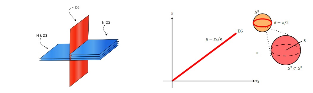
where are the generators in a -dimensional irreducible representation. All the classical fields are vanishing for . The VEVs are solution to the Nahm’s equations [19, 20, 21] that arise as conditions for the defect to preserve half of the original supersymmetry [22]. The four-dimensional conformal group of SYM is reduced to the three-dimensional one by the presence of the defect and the R-symmetry group is broken down to . The full superconformal group preserved by the defect is . The field theory configuration has a holographic dual realized by D3 branes intersected by a single probe D5 brane which in the near horizon limit warps an geometry inside the background generated by the D3 branes [23, 24, 25]. There is also a background gauge field flux of units through the sphere, meaning that of the D3 branes get dissolved into the D5 brane, as shown in Figure 2. The probe brane has worldvolume coordinates , it is tilted with an angle, that depends on , respect to the boundary of located at
| (1.2) |
and sits at the equator of the sphere.
Since the defect breaks part of the conformal symmetry, one-point functions of composite operators can be non-vanishing already at tree-level [26], as analyzed in [27, 28] for chiral primary operators in the defect set-up with units of flux. Furthermore, two-point functions of operators with unequal scaling dimension can be non-vanishing [29]. Using the tool of integrability, it was possible to derive a closed formula for tree-level one-point functions of non-protected operators in the sub-sector of SYM for any [30, 31], then generalized to higher loop orders [32] and to extend it to the sector [33] as well as the full scalar sector [34], see [35] for a review. One-point functions of composite operators have been recently analyzed in the and cases using the supersymmetric localization technique in [36, 37].
Compared to the standard AdS/CFT scenario, the defect that we are considering is characterized by the presence of a novel parameter , that on the field theory side controls the vevs of the scalar fields. In [17, 27], was suggested to consider a certain double scaling limit which consists of letting and subsequently sending and , the ’t Hooft coupling constant, to infinity (but with ) in such a way that the ratio can be taken fixed and small. Since , the supergravity approximation is reliable and for certain observables the results on the field theory and the string theory side of the correspondence organize in power series of , enabling the gauge-gravity comparison. Positive tests of the AdS/CFT correspondence in the D3-D5 defect set-up where both supersymmetry and conformal symmetry are partially broken have been performed in the double scaling limit for one-point functions of chiral primaries both at tree-level and one-loop[38, 39].
A highly non-trivial matching between gauge and string results for these operators has been achieved also in a different domain-wall version of described by a D3-D7 probe system, where all the supersymmetries are broken [28, 40, 41, 42, 43], see [44] for a recent review. Moreover, an agreement between gauge and string theory calculations in the D3-D5 set-up employing the double
scaling limit was found for a single Wilson line [17, 45], a pair of Wilson lines [46], and a circular Wilson loop in [47], for a small value of the coupling with the scalars and small distance from the defect, and in [48] where the double scaling limit was performed without restrictions on and on the distance from the interface. A positive check in the D3-D7 system has been performed for the Wilson line in [49].
Focusing on a circular Wilson loop of radius placed at on a plane parallel to the defect in the D3-D5 brane system, it has been shown in [48] that it experiences a first-order phase transition of Gross-Ooguri type (GO-like). The disk solution, which is the minimal surface in the theory without the defect, dominates when the operator is far from the interface. On the other hand, the cylindrical string solution, connecting the boundary loop with the probe D5-brane, is favorite below a certain critical distance from the defect.
In this work, we study the gravity dual of the two concentric circular Wilson loops correlator in the defect version of SYM theory. We will handle a complicated pattern of saddle-point configurations that are dominant in different regions of the parameter space describing the solutions. Besides the two saddle-points given by the disk-disk or the connected configuration between the circles, the minimal area configuration in the defect set-up can be given by two connected cylindrical surfaces attached to the boundary of AdS and ending on the D5 brane, or we can also have an intermediate case with a cylindrical surface for one of the loops and a disk for the other one. In the single circle case, the cylindrical surface attached to the defect can be described in terms of three parameters: , the coupling of the loop with the scalars, and . Since the defect preserves a subgroup of the original four-dimensional conformal group, the Wilson loop expectation value will depend on and only through their ratio. If two circles are considered, in addition to we can have two different couplings with the scalars, and , two different radii for the circles, and , and two different positions along that we indicate as and , where is the separation between the two loops. Thus, the parameter space describing the different saddle-points is enlarged. To simplify the problem, we will focus on the equal radii case. We will study the different sets of transitions à la Gross-Ooguri between different types of minimal surfaces and how they depend on the numerous parameters of the setting. This paper is organized as follows. In sec. 2 we find a new way to parametrize the connected solution between two circles and we analyze the allowed region of variation for the new parameters. This will make easier the comparison with the connected worldsheet solution to the defect, given in [48]. In sec. 3, we describe the feasible pattern of phase transitions occurring when we vary the parameters, focusing on some illustrative scenarios. At the end of this section, we investigate the possibility that the connected solution between the loops is intersected by the defect. A series of appendices complete the paper.
2 Connected solution between two circles
2.1 New parametrization for the “undefected” solution
The parametrization for the connected string solution between two concentric circles with different coupling with the scalars and radii has been carried out in [12]. Here, the parametrization of the relevant quantities as the renormalized action , the angular separation , and the distance between the two circles , is given in terms of two independent parameters and that have to be real and satisfy the condition . In the presence of the defect, another saddle-point, given by two separate cylindrical surfaces that start from the boundary of AdS and attach to the D5-brane, contributes to the evaluation of the correlator between the two circles. The exact solution for the cylindrical minimal area was found in [48]. In the following, it is more convenient to reparametrize the standard connected solution between the loops to simplify the comparison with the cylindrical surfaces, that will be the object of the analysis in sec 3. The Euclidean metric of is parametrized in Poincarè coordinates as
| (2.1) |
where denotes the metric of a 2-spheres in the . If we consider the ansatz for the minimal surface used in [12, 9]
| (2.2) |
we immediately recognize that it is the same string embedding used for the connected solution to the defect. In particular, we can find the minimal area between the two circles taking as a generic function of , without using the gauge choice . The exact geometric solution for the minimal surfaces described by this ansatz has been found in [48], and its embedding in is given by
| (2.3) |
where is the spatial worldsheet parameter, , and are integration constants and is an auxiliary function. Following [48], we can define in terms of as
| (2.4) |
with
| (2.5) |
such that
| (2.6) |
where is the Jacobi amplitude, and are the incomplete elliptic integral of first and third kind with elliptic modulus , respectively, defined in Appendix A. Here, is defined as
| (2.7) |
and
| (2.8) |
is a positive integration constant that appears in the first integral of . The constraint leads to two different ranges of variation for the couple of parameters :
| (2.9) |
Notice that , and in (2.1) satisfy the boundary conditions
| (2.10) |
The parametric solution in (2.1) draws a sub-manifold inside the following in :
| (2.11) |
This surface intersects the boundary of at , reaching it again at
| (2.12) |
In fact, for this value of the spatial world-sheet parameter
| (2.13) |
with
| (2.14) |
where and are the complete elliptic integrals of first and third kind. We still have to impose the following Dirichlet boundary conditions in
| (2.15) |
being the separation between the two circles. Notice that with respect to the solution given in [48], we are considering as an increasing function of . Thus, the solution for has a different sign here. Requiring to have at a circle of radius , we find
| (2.16) |
Imposing the last boundary condition in
| (2.17) |
one finds
| (2.18) |
The boundary condition in for the angle on the determines the constant
| (2.19) |
In we have to impose
| (2.20) |
where and are the different values of the scalar coupling at the boundary of for the two circles. We can define the angular separation between the loops as
| (2.21) |
where . Due to the R-symmetry, only the the angular separation is important and not the individual values of the couplings with the scalars.
2.2 Allowed region for the parameters
To have a more compact notation, it is possible to introduce the auxiliary parameter
| (2.22) |
By construction has to satisfy the following constraints
| (2.23) |
One can use (2.21) to determine in terms of and
| (2.24) |
The separation distance can be written as a functions of the angle and of the modular parameter using (2.18) and (2.14)
| (2.25) | ||||
The bounds on given in (2.23), precisely ensure the positivity of the expression in the square root in (2.25), and determine an upper and a lower limiting values for that we denote as and , respectively. In particular, solves the equation
| (2.26) |
while is a solution of
| (2.27) |
Fixing , one can obtain the corresponding values for and such that no solution exists for or . These bounds exposed above depict an allowed region of parameters that we show in Figure 3.

Now, we want to analyze how the separation distance behaves as approaches the two extrema and . When , we can use the following expansion for
| (2.28) |
where is a positive coefficient. We can use the expression of in terms of and given in the first line of (2.25), expanding around we find
| (2.29) |
Thus, we can conclude that the separation distance goes to zero as approaches . Notice that the coefficient in (2.28) can be determined by solving (2.24) perturbatively, getting
| (2.30) |
When , goes to and it is easy to see that goes to zero since the coefficient in the square root of (2.25) vanishes while
| (2.31) |
Thus, the distance between the loops is zero when approaches , it increases as is lowered, it reaches a maximum and it starts to decrease to be again zero at . From this analysis, it is clear that cannot be a monotonic function of , meaning that we cannot invert (2.25) to get as a function of and . Therefore, the two independent parameters that we use to describe the connected solution are and .

2.3 The area of the connected solution
The action of the connected minimal surface between the two circles is
| (2.32) |
Since it diverges as the world-sheet approaches the boundary, we have to regularize it imposing the boundary conditions and . Expanding for small , we have
| (2.33) |
| (2.34) |
Thus, the action becomes
| (2.35) |
Removing the divergent piece proportional to the perimeter of the two circles, the expression for the renormalized action takes the form
| (2.36) |

All the relevant quantities can be parametrized in terms of and . It is interesting to analyze the behavior of the area for the two boundary values of . Thus, it is more convenient to rewrite the as a function of and
| (2.37) |
When , using (2.28), we find
| (2.38) |
Since the combination is always negative for , we can conclude that the renormalized action diverges to as approaches . We can get the short-distance asymptotics of the action using the expansion for given in (2.29)
| (2.39) |
It exhibits a Coulombic behavior and diverges when the two circles coincide. If , which corresponds to the case, we recover the same result found in eq. (2.32) of [9] (notice that there is a difference of a factor coming from how we normalized the action).
If , the renormalized action assumes the finite value
| (2.40) |
In Figure 5, we have plotted the allowed region of parameters, given by the conditions in (2.23), in the plane corresponding to . This region collapses to a point when , meaning that no connected solution between the two circles exists for this value of the angle. Moreover, is a solution for the equation [12]
| (2.41) |
that corresponds to the condition for the two Wilson loops to have common supersymmetries. In this case, we have two separate domes that interact by the exchange of supergravity fields [50].
The area of the connected solution as a function of the separation distance for different values of the angular separation is presented in Figure 6. For each , there is always a maximal distance at which the connected solution starts to exist. If we decrease from its maximum, we find two different branches of solutions that terminate at . The upper one is always subdominant and its end-point at corresponds to The lower and dominant branch is given by values of that run from to the maximal value of the separation.

There is always a critical at which the renormalized action is equal to the area of two disconnected spherical domes. Thus, for values of greater than the critical one, the dominant solution is given by two spherical domes. Below the critical separation distance, the configuration with the minimal area is the connected solution. We can numerically determine both the critical and the maximal value of . For , we have verified that they coincide with the results given in [9], namely
| (2.42) |
3 Phase transitions in the presence of the defect
The study of a single circular Wilson loop in SYM theory in the presence of a defect, considered in [47, 48], can be extended to the case in which two circles are inserted in the set-up realized by the D3-D5 probe-brane intersection. Besides the two different saddle points described in sec. 2.3, the minimal area configuration can be given by two connected cylindrical surfaces stretched from the boundary of AdS to the defect or a cylindrical surface for one of the loops and a disk for the other one. The two concentric loops are placed on planes parallel to the defect at a distance and , respectively. For simplicity, we consider the case in which the circles have the same radius , namely . The two Wilson loops can couple with the scalars and of the theory with different angles and they are opposite oriented in space-time11 1 No connected solution between the circles is allowed if they have the same orientation [13, 12, 14]
| (3.1) |
where each loop is parametrized by
| (3.2) | ||||
| (3.3) |
The first loop, located at , will have an internal angle while for the second one, at , the coupling with the scalar will be given by . The parameters that describe the solutions are
| (3.4) |
As anticipated, when the defect is present we have richer situations with respect to the standard Gross-Ooguri phase transition between the two circles. We expect that when both circles are far away from the defect , the picture is the one described in the previous section. Depending on , the dominant solution will be given by the connected surface between the contours or it will consist of two disconnected domes. If we get closer to the defect, we can have a greater variety of configurations for the minimal area since the defect opens the possibility to have also cylindrical surfaces that start from the boundary of AdS and attach to the D5-brane.
To investigate the possible configurations that can dominate for different values of , we can start by fixing all the independent parameters in (3.4) except , in such a way that the first loop is kept at a fixed distance from the defect while letting the second one to move away from it. In our parametrization the second circle is placed at a distance from the defect given by
| (3.5) |
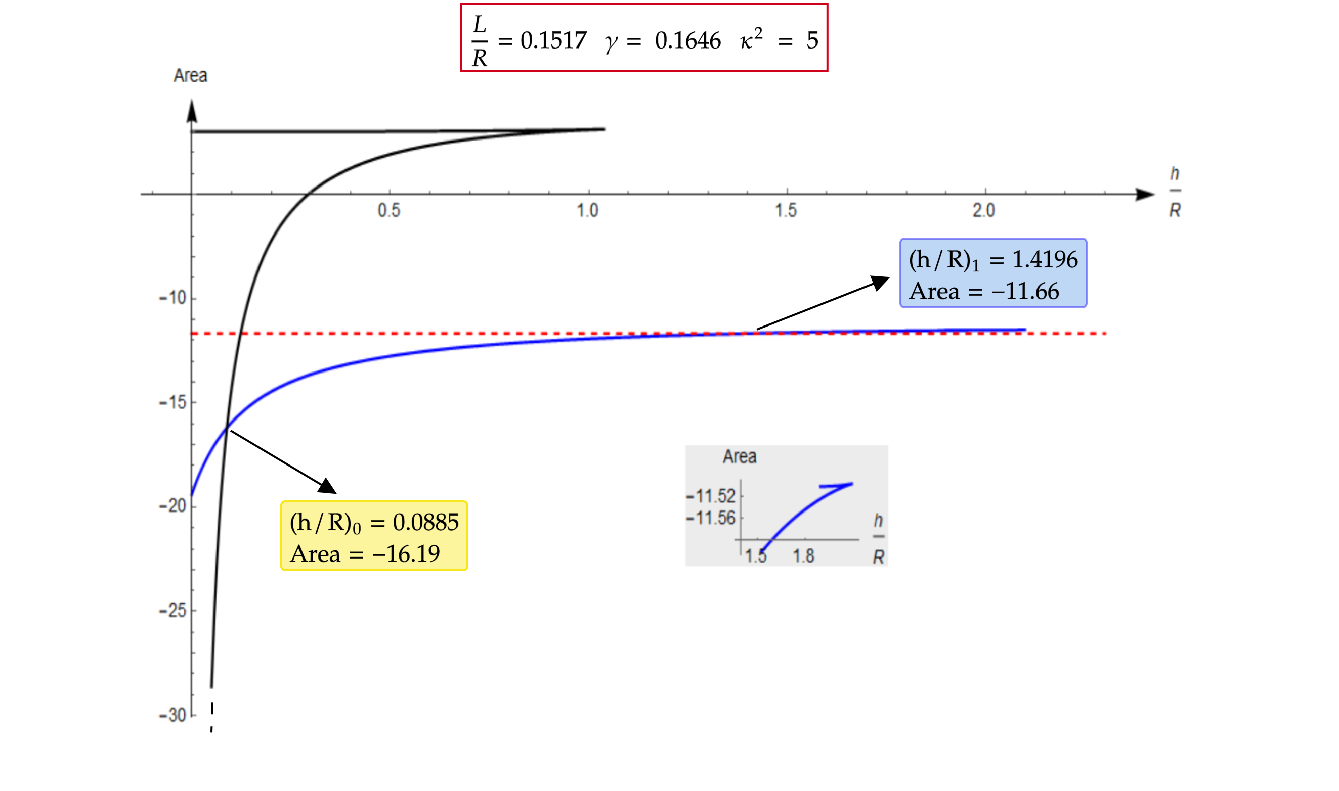
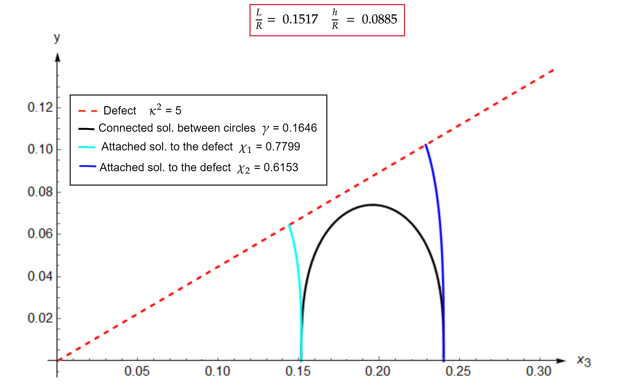
In Figure 7, we plot the different types of solutions that are dominant for different values of . We have chosen for the scalar couplings and the flux the values and . To show the behavior of the action as a function of , we have also fixed the distance of the first loop from the defect . For this value, the cylindrical configuration extending from the boundary of AdS to the D5-brane is the solution with the minimal area for the first loop and, since we do not vary , the value of does not change. Approaching from infinity the defect with the second loop, we encounter a value of at which the cylindrical solution starts to exist also for the second circle, and at its area becomes equal to the area of the dome. Thus, for the minimal area configuration for the two loops is given by two cylindrical surfaces, one for each circle, attached to the defect. We refer to this solution as the attached-attached configuration. Keeping to decrease , we reach the value at which the area of the two cylindrical surfaces (blue curve in Figure 7), becomes equal to the area of the connected configuration between the circles (black curve). This configuration is visualized in Figure 8. For smaller values of the separation distance, the latter becomes dominant with respect to the former. In the example reported in Figure 7, the connected solution becomes dominant for . We can summarize as follows, in terms of the separation distance, the two different transitions that can be present in the two circles correlator when a defect is inserted in the theory
- 1)
transition between the connected and the attached-attached to the defect configuration
- 2)
transition between the attached-attached and the attached-dome configuration.
In the following, we will study different values of the physical parameters that will lead to different combinations of GO-like phase transitions.

3.1 Different distances from the defect
In Figure 9, we analyze what happens if we put the first circle at different positions with respect to the defect, without changing , and . The green and blue curves correspond to the area of the attached-attached configuration for two different values of . When the first loop is closer to the defect (green curve), we find two different types of Gross-Ooguri transitions as described before. For small values of , the dominant solution is the connected one (black curve). Increasing the separation between the loops, we have a value of where the connected solution and the attached-attached configuration have the same area, corresponding to the black curve crossing the green one in Figure 9 . If we increase further , the attached-attached configuration becomes the minimal one, but the area of the cylindrical surface for the second circle becomes less negative since we are moving the loop away from the defect. When , the second Gross-Ooguri transition to the attached-dome configuration takes place. That corresponds to have the cylindrical surface for the first circle, whose position is kept fixed, and the dome solution for the second one. In Figure 9, this transition occurs at the crossing point between the dashed-green line and the continuous green curve. When we increase , the sum of the areas of the two cylindrical solutions becomes less negative. Thus, the only relevant transition may be between the connected and the attached-dome configuration since there are no values of for which the attached-attached solution is dominant. This case is shown in Figure 9 by the blue curve. The black curve does not change as we vary , since it depends only on and .

There should be an intermediate case that interpolates between the two different behaviors shown in Figure 9 and which is characterized by a certain value of , denoted as , at which the connected, the attached-attached, and the attached-dome configurations have the same area for the same value of . We can summarize the different situations choosing different values for the distance from the defect, as follows
- •
there are two different types of transitions. At takes place the first one between the connected and the attached-attached configuration, while at the attached-dome solution becomes dominant (crossing between the cyan continuous curve and the dashed one in Figure 10).
- •
in this case , namely the connected solution is dominant until the separation between the circles reaches a value at which this saddle-point has the same area as the attached-attached and the attached-dome solutions. We refer to this particular configuration as the triple point, since the three solutions have the same area for the same value of . Keeping to increase , the solution with the minimal area is given by a cylindrical surface attached to the defect for the loop located at , and the dome for the second one.
- •
the attached-attached configuration is never dominant and the only relevant transition is the one between the connected and the attached-dome solutions.
3.2 Transitions for different fluxes and angles

In Figure 11, we plot different types of solution for fixed and , varying the flux. The connected configuration does not change since it is independent on . For the values of and considered, the cylindrical solution for the first circle is dominant with respect to the dome. The transition between the connected and the attached-attached configuration is possible and it occurs at a value of the separation distance between the loops, given by , that decreases as the flux grows since becomes more negative. On the other hand, the space of parameters of the cylindrical solution is enlarged by increasing the flux (see fig. 4 of [48]). Thus, the value where occurs the transition to the attached-dome configuration, increases with the flux. When grows, the attached-attached solution dominates for a larger range of values of , because the slope of the brane becomes smaller and the defect gets closer to the boundary. As we increase the flux, it is energetically preferred for the system to settle in the attached-attached solution.

In Figure 12, for fixed varying and , we plot the separation distance between the loops at which the first relevant transition occurs. For small values of , the first relevant transition is the one between the connected and the attached-attached configuration. A change in the slope of the curves takes place at , namely when the triple point is reached. For , the attache-attached solution is never dominant and the first relevant transition is between the connected and the attached-dome configuration. In this plot, it is better displayed that, as the flux is increased, the transition between the connected and the attached-attached solution occurs at smaller for equal values of . Moreover, we can also notice that increases with the flux. All the curves stop when the loop closer to the defect is placed at a value of such that the cylindrical surface attached to the defect becomes less preferred with respect to the dome. Thus, for larger , the only relevant transition is between the connected surface and the two domes, as in the standard GO case. For , it happens at , which is the value at which all the curves stop in Figure 12. These considerations are displayed in Figure 13, where we plot for fixed , and the scheme of the possible transitions in the plane of the parameters .

Now, we want to analyze what happens if we exchange and . Contrary to the case without the defect, where only the difference between the two is relevant, here also the value of the single angle is important. This is because the defect breaks the original R-symmetry of SYM theory to . In Figure 14, we have fixed two values for the coupling with the scalars, , and . The connected solution (black curve) depends only on and it is invariant under the exchange of and .

We can choose a value for such that no cylindrical surface exists for the loop with the smaller angle, while for the second circle the cylindrical surface exists and its area is smaller than the area of the dome, as is shown in Figure 15. If , we can have the following situations depending on the value of :
-
the connected solution is the dominant one.
-
the configuration with the minimal area is the dome-attached solution, represented in Figure 14 by the blue curve. The loop which is closer to the defect is characterized by the angle . Thus, only the dome solution is possible at the chosen value of , while for the circle with the cylindrical surface is dominant with respect to the dome.
-
at the area of the cylindrical surface for the second circle becomes equal to -1 and the dome-dome configuration, represented in Figure 14 by the dashed-red line, is the one with the minimal area. Compared to the case without the defect, the transition to the dome-dome configuration occurs at a larger value of the separation distance.
If we exchange the values of the angles in such a way that , we have only two possible situations:
-
the connected solution is the dominant one.
-
the configuration with the minimal area is the attached-dome solution, given in Figure 14 by the cyan line. This configuration has a constant area since we are moving away from the defect the loop whose solution, for this range of parameters, is the dome. Thus, its area remains constant and equal to -1 as we vary .
In Figure 14, we can notice that exchanging and also the value of at which the connected solution stops to be dominant changes. Moreover, we can choose different pairs of and that give the same , but we do not expect the same result for the values of and , as shown in Figure 16. When and are larger, the attached-attached configuration can exist and dominate for larger values of .


3.3 String-brane crossing
In this section, we will inspect whether or not the connected solution between the loops can be intersected by the defect. If this is feasible, the transition between the connected and the attached-attached configuration can happen before the latter becomes dominant with respect to the former and a zero-order phase transition can occur.
The D5-brane has the following profile inside [17, 27]
| (3.6) |
where and are two constant values. If the defect is tangent to the connected solution in , the following conditions have to be satisfied
| (3.7) | ||||
| (3.8) |
Eq. (3.7) has a unique solution in the interval when corresponds to the minimum of the function . Thus, we have a further condition to impose
| (3.9) |
which can be seen, for fixed values of and the angles, in Figure 17.

This derivative is always positive in the interval , where it does not possess a minimum. Solving eq. (3.8), we can express as a function of and as
| (3.10) |
Since has to be positive, we assume . The condition gives an additional constraint on the values that can assume, namely . Combining eqs. (3.9) and (3.7), we can determine the critical value of the flux at which the connected solution touches the brane
| (3.11) |
where we have used the equation of motion for
| (3.12) |
Due to , is positive 22 2 With we indicate the derivative of respect to . and . Using eq. (3.7), we get an expression for the critical distance of the first circle from the defect at which the worldsheet stretching between the two circles and the brane touch each other.
The explicit form of and is displayed in appendix C. The critical parameters can be expressed as functions of , and (that corresponds to a specific value for ). Thus, as we vary , the values change.

Alternatively, we can fix the two angles, the distance from the defect of the first circle with scalar coupling , and numerically determine the set of values at which occurs the crossing. For or , keeping fixed the other parameters, the connected configuration remains below the brane without crossing. Increasing the distance from the defect of the connected solution, at fixed angles on the , and grow. Notice that to have a brane-string intersection in the part of the space, it is necessary that the angles and belong to different hemispheres, namely and . The touching may take place at a value such that the connected solution is no longer dominant. In Figure 18 we show that, for the values of the parameters considered, the transition between the connected solution and the attached-attached configuration takes place for a separation distance between the circles smaller than . Proving in general that the touching always happen when the connected configuration has no longer the minimal area is a hard task, due to the large parameter space involved. Thus, to be sure to avoid the string-brane crossing, we take and in the same hemisphere.
Moreover, we can focus the case that corresponds to have no motion of the string in the . It makes sense to analyze the problem of the string-brane touching for this value of only when the angles are both equal to . Otherwise, the brane and the defect are not tangent in the part of the space. The condition in eq. (3.8) is always satisfied if , since . Therefore, we have to impose only the two constraints related to the touching in the part of the space, given in eq. (3.7) and (3.9). Through these conditions, we can fix the value of and for which the connected solution and the defect become tangent. Keeping fixed and , we can find different values of and at which the connected solution touches the probe brane. Conversely, in the case at a certain value of corresponds only a possible value for and at which the touching occurs. In fact, there are other values of these parameters that satisfy the conditions in eq. (3.7) and (3.9) in principle, but not the one in eq. (3.8) regarding the sphere. In Figure 19, varying the distance from the defect of the first loop and for fixed , and , we plot the values of at which the transition between the connected and the attached-attached configuration occurs (blue line). The red curve displayes the values of corresponding to the connected solution being tangent to the defect. In the case considered, which is also investigated in Figure 10, the transition always happen before the touching. We have numerically verified that this also happens for other values of the flux.

4 Conclusions and Outlook
We have further made a study of the string theory dual of the two concentric circular Wilson loops correlator in a defect version of SYM, in the equal radii case. The defect is realized as a probe D5 brane in the gravity side of the AdS/CFT correspondence. We analyzed how the GO phase transition [6], that takes place in the correlator of two circular Wilson loops, is modified when a defect is inserted. When two circles are considered, the parameter space characterizing the different saddle-points that contribute to the evaluation of the correlator, is even richer than the single circle case. It is given by , , and , and , namely the distance of the first loop from the defect, the separation distance between the loops, their angular positions in , and the flux, respectively. Thus, the Wilson loops correlator can undergo new types of GO-like phase transitions whose analysis becomes more intricate. The standard GO-transition takes place when the separation distance between the two circles gets larger and is above a critical value at which the connected worldsheet solution between the two contours splits into two disjointed domes that have a smaller area, and that continue to interact through the exchange of light supergravity modes. In our case, this picture remains valid when we are far away from the defect, but when the circles get closer to it new minimal surface solutions are present. In particular, for some values of the parameters, the configuration with the minimal area can consist of two cylindrical surfaces attached to the defect or of one cylindrical surface for one of the contours, and a dome for the second one. We have studied the possible transitions between different minimal surface configurations in different regions of the parameter space. The solution corresponding to the string worldsheet connecting the two loops found in [12] has been rewritten in terms of new parameters, to easily make a comparison between different saddle-points in the defect theory. We found that, if the first loop is placed at a non-zero distance from the defect and the value of is small, the dominant solution is the connected one. Increasing the separation distance between the loops, the other conceivable configurations mentioned above can become dominant, depending on the values of the other parameters of the system. We have also examined the case concerning the ”string-brane crossing”, which contemplates the possibility for the connected solution between the circles to touch and then intersect the defect brane. In this case, the transition between the connected solution and two separate cylindrical surfaces attached to the defect can happen before the latter configuration has a smaller area than the former, resulting in a zero-order phase transition. In [48], it was shown that, for a single circle, the dome geometry becomes less energetically preferred with respect to the cylindrical surface before touching the defect, i.e. the GO-like transition always happens before the string-brane crossing. In our case, since we have a larger parameter space, the discussion is more involved. We avoid this phenomenon by placing the string endpoints in the same hemisphere of the . In principle, non-trivial string three-point functions could also enter the game, describing new connected minimal surfaces with three holes, one of which lying on the defect. This configuration involves string interactions and has an additional power of in the gauge theory language. Thus, it is a higher order effect respect to the classical string solutions that we considered in this work. Moreover, we expect this configuration’s analysis to be very involved and we leave the study of its properties to future work. The two circles correlator’s study in a defect version of SYM can be extended to the case of circular Wilson loops with different radii, obviously increasing the dimensions of the parameter space. As pointed out in [51], the correlator of two circles in parallel planes separated by a distance are conformally related by a stereographic projection to coincident circles with different radii. When the defect is present, the conformal map should also involve the defect itself, which spoils part of the conformal invariance of the original theory. As a future development, it would be interesting to analyze the effect of the stereographic projection on the defect and how this conformal map works in the defect CFT (dCFT) case. Moreover, by virtue of the enticing results achieved in [37], it would be worthwhile to compute in the dCFT the expectation value of a circular Wilson loop operator and the two-circles correlator, in the BPS case, using the localization technique. Also, the Wilson loops correlator in higher representations, in particular the symmetric and antisymmetric ones [52, 53], can be inspected in this new defect set-up.
Acknowledgements
Special thanks go to Luca Griguolo, Domenico Seminara, and Diego Trancanelli for participating in the early stages of this work and many interesting discussions. It is also our pleasure to thank D. Correa and C. Kristjansen, for useful discussions. The work of S.B. is supported by ” Fondazione Angelo Della Riccia” and in part by the research fellowship ”Non-perturbative methods in quantum field theory: holography and beyond” at Università degli Studi di Firenze, R.S was financed in part by the Coordenação de Aperfeiçoamento de Pessoal de Nível Superior - Brasil (CAPES) - Finance Code 001.
Appendix A Jacobi elliptic functions and elliptic integrals
In this paper we work with the standard Jacobi elliptic functions and elliptic integrals defined along the lines of [54]. We use the incomplete elliptic integrals
| (A.1) | ||||
| (A.2) | ||||
| (A.3) |
of the first, second and third kind, respectively. The complete elliptic integrals are defined as
| (A.4) |
We also use the Jacobi amplitude which is the inverse of
| (A.5) |
The Jacobi elliptic functions are defined as
| (A.6) |
such that and . The reciprocals of the latter functions are
| (A.7) |
Appendix B Parametrization of the connected solution
We check that our parametrization reproduces the results of [12] where the classical connected solution is written down in terms of the two parameters and :
| (B.1) | ||||
| (B.2) | ||||
| (B.3) |
To verify that equation (B.2) corresponds to our result for given in (2.21), we take the definition of and
| (B.4) |
where and are the two constants of motion found in [12]. It is easy to check that they correspond exactly to and , which are the positive integration constants given in [48]
| (B.5) |
The expression for , for the equal radii case, in our notation is
| (B.6) |
Therefore, we find that and can be written in terms of and in the following way
| (B.7) |
If we rephrase the bounds on and
| (B.8) |
in terms of and , we get exactly the same bounds on given in (2.23). If we perform the substitution of (B.7) in (B.2) using the identity
| (B.9) |
we get for the expression given in (2.21). The same can be done for the action and substituting (B.7) in equation (B.3) we get exactly (2.36) using the identity
| (B.10) |
In order to verify that our solution reproduces also the form for , we notice that
| (B.11) |
where in equal radii case. The l.h.s of the equation above is equal to the integral
| (B.12) |
that, through the change of variable in (B.4), defines . This integral is obtained parametrizing and as
| (B.13) |
where . Since for us
| (B.14) |
if we compare (B.13) with (2.1), where , we recognize that
| (B.15) |
Thus,
| (B.16) |
and is zero at or . The maximum value of , denoted as , is reached when assumes its minimal, namely at
| (B.17) |
Performing the change of variables (B.15) in (B.12), we get
| (B.18) |
Using the expression for the first integral for derived in [48]
| (B.19) |
and the fact that is negative if , the previous integral simplifies to
| (B.20) |
Performing the integral, we get
| (B.21) |
Finally, we have shown that also can be perfectly mapped to our parametrization.
Appendix C Explicit solution for the string-brane crossing
We can use a combination of conditions (3.9) and (3.7) to express as
| (C.1) |
where we have also used that
| (C.2) |
Notice that , defined in eq. (2.8), can be expressed as a function of and
| (C.3) |
The critical value of is derived from eq. (3.7) using the explicit form of and given in eq. (2.1) and it reads
| (C.4) |
References
- [1] J. M. Maldacena, Wilson loops in large N field theories, Phys. Rev. Lett. 80 (1998) 4859–4862. arXiv:hep-th/9803002, doi:10.1103/PhysRevLett.80.4859.
- [2] S.-J. Rey, J.-T. Yee, Macroscopic strings as heavy quarks in large N gauge theory and anti-de Sitter supergravity, Eur. Phys. J. C22 (2001) 379–394. arXiv:hep-th/9803001, doi:10.1007/s100520100799.
- [3] J. K. Erickson, G. W. Semenoff, K. Zarembo, Wilson loops in N=4 supersymmetric Yang-Mills theory, Nucl. Phys. B582 (2000) 155–175. arXiv:hep-th/0003055, doi:10.1016/S0550-3213(00)00300-X.
- [4] N. Drukker, D. J. Gross, An Exact prediction of N=4 SUSYM theory for string theory, J. Math. Phys. 42 (2001) 2896–2914. arXiv:hep-th/0010274, doi:10.1063/1.1372177.
- [5] V. Pestun, Localization of gauge theory on a four-sphere and supersymmetric Wilson loops, Commun. Math. Phys. 313 (2012) 71–129. arXiv:0712.2824, doi:10.1007/s00220-012-1485-0.
- [6] D. J. Gross, H. Ooguri, Aspects of large N gauge theory dynamics as seen by string theory, Phys. Rev. D58 (1998) 106002. arXiv:hep-th/9805129, doi:10.1103/PhysRevD.58.106002.
- [7] D. E. Berenstein, R. Corrado, W. Fischler, J. M. Maldacena, The Operator product expansion for Wilson loops and surfaces in the large N limit, Phys. Rev. D59 (1999) 105023. arXiv:hep-th/9809188, doi:10.1103/PhysRevD.59.105023.
- [8] A. Bassetto, L. Griguolo, F. Pucci, D. Seminara, S. Thambyahpillai, D. Young, Correlators of supersymmetric Wilson-loops, protected operators and matrix models in N=4 SYM, JHEP 08 (2009) 061. arXiv:0905.1943, doi:10.1088/1126-6708/2009/08/061.
- [9] K. Zarembo, Wilson loop correlator in the AdS / CFT correspondence, Phys. Lett. B459 (1999) 527–534. arXiv:hep-th/9904149, doi:10.1016/S0370-2693(99)00717-0.
- [10] P. Olesen, K. Zarembo, Phase transition in Wilson loop correlator from AdS / CFT correspondence (2000). arXiv:hep-th/0009210.
- [11] H. Kim, D. K. Park, S. Tamarian, H. J. W. Muller-Kirsten, Gross-Ooguri phase transition at zero and finite temperature: Two circular Wilson loop case, JHEP 03 (2001) 003. arXiv:hep-th/0101235, doi:10.1088/1126-6708/2001/03/003.
- [12] D. H. Correa, P. Pisani, A. Rios Fukelman, Ladder Limit for Correlators of Wilson Loops, JHEP 05 (2018) 168. arXiv:1803.02153, doi:10.1007/JHEP05(2018)168.
- [13] K. Zarembo, String breaking from ladder diagrams in SYM theory, JHEP 03 (2001) 042. arXiv:hep-th/0103058, doi:10.1088/1126-6708/2001/03/042.
- [14] D. Correa, P. Pisani, A. Rios Fukelman, K. Zarembo, Dyson equations for correlators of Wilson loops, JHEP 12 (2018) 100. arXiv:1811.03552, doi:10.1007/JHEP12(2018)100.
- [15] O. DeWolfe, D. Z. Freedman, H. Ooguri, Holography and defect conformal field theories, Phys. Rev. D66 (2002) 025009. arXiv:hep-th/0111135, doi:10.1103/PhysRevD.66.025009.
- [16] J. Erdmenger, Z. Guralnik, I. Kirsch, Four-dimensional superconformal theories with interacting boundaries or defects, Phys. Rev. D66 (2002) 025020. arXiv:hep-th/0203020, doi:10.1103/PhysRevD.66.025020.
- [17] K. Nagasaki, H. Tanida, S. Yamaguchi, Holographic Interface-Particle Potential, JHEP 01 (2012) 139. arXiv:1109.1927, doi:10.1007/JHEP01(2012)139.
- [18] M. de Leeuw, A. C. Ipsen, C. Kristjansen, M. Wilhelm, Introduction to integrability and one-point functions in 4 supersymmetric Yang–Mills theory and its defect cousin, Les Houches Lect. Notes 106 (2019) 352–399. arXiv:1708.02525, doi:10.1093/oso/9780198828150.003.0008.
- [19] W. Nahm, A Simple Formalism for the BPS Monopole, Phys. Lett. 90B (1980) 413–414. doi:10.1016/0370-2693(80)90961-2.
- [20] D.-E. Diaconescu, D-branes, monopoles and Nahm equations, Nucl. Phys. B503 (1997) 220–238. arXiv:hep-th/9608163, doi:10.1016/S0550-3213(97)00438-0.
- [21] N. R. Constable, R. C. Myers, O. Tafjord, The Noncommutative bion core, Phys. Rev. D61 (2000) 106009. arXiv:hep-th/9911136, doi:10.1103/PhysRevD.61.106009.
- [22] D. Gaiotto, E. Witten, Supersymmetric Boundary Conditions in N=4 Super Yang-Mills Theory, J. Statist. Phys. 135 (2009) 789–855. arXiv:0804.2902, doi:10.1007/s10955-009-9687-3.
- [23] A. Karch, L. Randall, Locally localized gravity, JHEP 05 (2001) 008, [,140(2000)]. arXiv:hep-th/0011156, doi:10.1088/1126-6708/2001/05/008.
- [24] A. Karch, L. Randall, Open and closed string interpretation of SUSY CFT’s on branes with boundaries, JHEP 06 (2001) 063. arXiv:hep-th/0105132, doi:10.1088/1126-6708/2001/06/063.
- [25] A. Karch, L. Randall, Localized gravity in string theory, Phys. Rev. Lett. 87 (2001) 061601. arXiv:hep-th/0105108, doi:10.1103/PhysRevLett.87.061601.
- [26] J. L. Cardy, Conformal Invariance and Surface Critical Behavior, Nucl. Phys. B240 (1984) 514–532. doi:10.1016/0550-3213(84)90241-4.
- [27] K. Nagasaki, S. Yamaguchi, Expectation values of chiral primary operators in holographic interface CFT, Phys. Rev. D86 (2012) 086004. arXiv:1205.1674, doi:10.1103/PhysRevD.86.086004.
- [28] C. Kristjansen, G. W. Semenoff, D. Young, Chiral primary one-point functions in the D3-D7 defect conformal field theory, JHEP 01 (2013) 117. arXiv:1210.7015, doi:10.1007/JHEP01(2013)117.
- [29] M. de Leeuw, A. C. Ipsen, C. Kristjansen, K. E. Vardinghus, M. Wilhelm, Two-point functions in AdS/dCFT and the boundary conformal bootstrap equations, JHEP 08 (2017) 020. arXiv:1705.03898, doi:10.1007/JHEP08(2017)020.
- [30] M. de Leeuw, C. Kristjansen, K. Zarembo, One-point Functions in Defect CFT and Integrability, JHEP 08 (2015) 098. arXiv:1506.06958, doi:10.1007/JHEP08(2015)098.
- [31] I. Buhl-Mortensen, M. de Leeuw, C. Kristjansen, K. Zarembo, One-point Functions in AdS/dCFT from Matrix Product States, JHEP 02 (2016) 052. arXiv:1512.02532, doi:10.1007/JHEP02(2016)052.
- [32] I. Buhl-Mortensen, M. de Leeuw, A. C. Ipsen, C. Kristjansen, M. Wilhelm, Asymptotic One-Point Functions in Gauge-String Duality with Defects, Phys. Rev. Lett. 119 (26) (2017) 261604. arXiv:1704.07386, doi:10.1103/PhysRevLett.119.261604.
- [33] M. de Leeuw, C. Kristjansen, S. Mori, AdS/dCFT one-point functions of the SU(3) sector, Phys. Lett. B 763 (2016) 197–202. arXiv:1607.03123, doi:10.1016/j.physletb.2016.10.044.
- [34] M. De Leeuw, C. Kristjansen, G. Linardopoulos, Scalar one-point functions and matrix product states of AdS/dCFT, Phys. Lett. B 781 (2018) 238–243. arXiv:1802.01598, doi:10.1016/j.physletb.2018.03.083.
- [35] M. de Leeuw, One-point functions in AdS/dCFT, J. Phys. A 53 (28) (2020) 283001. arXiv:1908.03444, doi:10.1088/1751-8121/ab15fb.
- [36] Y. Wang, Taming defects in = 4 super-Yang-Mills, JHEP 08 (08) (2020) 021. arXiv:2003.11016, doi:10.1007/JHEP08(2020)021.
- [37] S. Komatsu, Y. Wang, Non-perturbative defect one-point functions in planar super-Yang-Mills, Nucl. Phys. B 958 (2020) 115120. arXiv:2004.09514, doi:10.1016/j.nuclphysb.2020.115120.
- [38] I. Buhl-Mortensen, M. de Leeuw, A. C. Ipsen, C. Kristjansen, M. Wilhelm, One-loop one-point functions in gauge-gravity dualities with defects, Phys. Rev. Lett. 117 (23) (2016) 231603. arXiv:1606.01886, doi:10.1103/PhysRevLett.117.231603.
- [39] I. Buhl-Mortensen, M. de Leeuw, A. C. Ipsen, C. Kristjansen, M. Wilhelm, A Quantum Check of AdS/dCFT, JHEP 01 (2017) 098. arXiv:1611.04603, doi:10.1007/JHEP01(2017)098.
- [40] M. de Leeuw, C. Kristjansen, G. Linardopoulos, One-point functions of non-protected operators in the SO(5) symmetric D3–D7 dCFT, J. Phys. A50 (25) (2017) 254001. arXiv:1612.06236, doi:10.1088/1751-8121/aa714b.
- [41] A. Gimenez Grau, C. Kristjansen, M. Volk, M. Wilhelm, A Quantum Check of Non-Supersymmetric AdS/dCFT, JHEP 01 (2019) 007. arXiv:1810.11463, doi:10.1007/JHEP01(2019)007.
- [42] A. Gimenez-Grau, C. Kristjansen, M. Volk, M. Wilhelm, A Quantum Framework for AdS/dCFT through Fuzzy Spherical Harmonics on , JHEP 04 (2020) 132. arXiv:1912.02468, doi:10.1007/JHEP04(2020)132.
- [43] M. De Leeuw, T. Gombor, C. Kristjansen, G. Linardopoulos, B. Pozsgay, Spin Chain Overlaps and the Twisted Yangian, JHEP 01 (2020) 176. arXiv:1912.09338, doi:10.1007/JHEP01(2020)176.
- [44] G. Linardopoulos, Solving holographic defects, PoS CORFU2019 (2020) 141. arXiv:2005.02117, doi:10.22323/1.376.0141.
- [45] M. de Leeuw, A. C. Ipsen, C. Kristjansen, M. Wilhelm, One-loop Wilson loops and the particle-interface potential in AdS/dCFT, Phys. Lett. B768 (2017) 192–197. arXiv:1608.04754, doi:10.1016/j.physletb.2017.02.047.
- [46] M. Preti, D. Trancanelli, E. Vescovi, Quark-antiquark potential in defect conformal field theory, JHEP 10 (2017) 079. arXiv:1708.04884, doi:10.1007/JHEP10(2017)079.
- [47] J. Aguilera-Damia, D. H. Correa, V. I. Giraldo-Rivera, Circular Wilson loops in defect Conformal Field Theory, JHEP 03 (2017) 023. arXiv:1612.07991, doi:10.1007/JHEP03(2017)023.
- [48] S. Bonansea, S. Davoli, L. Griguolo, D. Seminara, Circular Wilson loops in defect = 4 SYM: phase transitions, double-scaling limits and OPE expansions, JHEP 03 (2020) 084. arXiv:1911.07792, doi:10.1007/JHEP03(2020)084.
- [49] S. Bonansea, K. Idiab, C. Kristjansen, M. Volk, Wilson lines in AdS/dCFT, Phys. Lett. B 806 (2020) 135520. arXiv:2004.01693, doi:10.1016/j.physletb.2020.135520.
- [50] S. Giombi, V. Pestun, R. Ricci, Notes on supersymmetric Wilson loops on a two-sphere, JHEP 07 (2010) 088. arXiv:0905.0665, doi:10.1007/JHEP07(2010)088.
- [51] N. Drukker, B. Fiol, On the integrability of Wilson loops in : Some periodic ansatze, JHEP 01 (2006) 056. arXiv:hep-th/0506058, doi:10.1088/1126-6708/2006/01/056.
- [52] T.-S. Tai, S. Yamaguchi, Correlator of Fundamental and Anti-symmetric Wilson loops in AdS/CFT Correspondence, JHEP 02 (2007) 035. arXiv:hep-th/0610275, doi:10.1088/1126-6708/2007/02/035.
- [53] J. Aguilera-Damia, D. H. Correa, F. Fucito, V. I. Giraldo-Rivera, J. F. Morales, L. A. Pando Zayas, Strings in Bubbling Geometries and Dual Wilson Loop Correlators, JHEP 12 (2017) 109. arXiv:1709.03569, doi:10.1007/JHEP12(2017)109.
- [54] M. Abramowitz, I. Stegun, Handbook of Mathematical Functions, fifth edition, Dover (1964), New York.