Variational optimization and data assimilation in chaotic time-delayed systems with automatic-differentiated shadowing sensitivity
Abstract
In this computational paper, we perform sensitivity analysis of long-time (or ensemble) averages in chaotic regime using the shadowing algorithm. We introduce automatic differentiation to eliminate the tangent/adjoint equation solvers used in the shadowing algorithm. In a gradient-based optimization, we use the computed shadowing sensitivity to minimize different long-time averaged functionals of a chaotic time delayed system by optimal parameter selection. In combined state and parameter estimation for data assimilation, we use the computed sensitivity to predict the optimal trajectory given information from a model and data from measurements beyond the predictability time. The algorithms are applied to a thermoacoustic model. Because the computational framework is rather general, the techniques presented in this paper may be used for sensitivity analysis of ensemble averages, parameter optimization and data assimilation of other chaotic problems, where shadowing methods are applicable.
Keywords:
Optimization , Time-delayed systems , Chaos , Data assimilation1 Introduction
Sensitivities are quantitative
measures of the response of model outputs to infinitesimal
changes in inputs, which are crucial to engineering design [1, 2]. They are employed
in parameter
estimation and model selection [3, 4], uncertainty quantification [5, 6], data assimilation [7, 8, 9]
and design and optimization (see [10, 11, 12, 13] for
recent reviews of the applications of sensitivity derivatives in different
engineering disciplines). With the growing ability
to simulate high-dimensional complex dynamics, much research
effort has been invested into commensurately improving sensitivity
analysis methods. Adjoints of mathematical models have been
developed and used successfully in many fields; for example,
adjoint sensitivity analysis in meteorology [14, 15],
aircraft design [16], systems biology [17], chemical kinetics [7], thermo-fluids [13], among others.
The adjoint method is generally used when the input parameter
space is high-dimensional. Tangent Linear Models (TLMs) and finite
difference methods are also used for sensitivity analysis
when the dimension of the input parameter space is small enough
that the cost of simulating the original dynamics repeatedly is not prohibitive.
In many of these applications, automatic differentiation (AD) has successfully replaced
the TLM or adjoint computations [18, 19]. For example, MITGCM [20], a popular
climate model uses OpenAD [21, 22], an
open source source-transformation AD software [23, 24, 25, 26]; and
Tapenade [27, 28] has replaced adjoint
differentiation in a few industrial-size numerical codes.
In recent times, simultaneous advances in simulation capabilities and computing power have led to a proliferation of scale-resolving simulations of chaotic systems [29, 30, 31, 32]. For many of the above target applications, the relevant observables, or outputs, in chaotic systems are statistically stationary or infinitely long-time averaged functions [30, 31, 32, 33, 34]. Useful gradients of ensemble averages, which are equal to infinite time averages in ergodic systems, cannot be obtained by time-averaging the instantaneous gradients in chaotic systems [35]. Indeed, in the infinite time limit, the time averages of the instantaneous gradients diverge despite that the ensemble averages of the functions may have a well-defined gradient. This is because the tangent space of a chaotic attractor is exponentially unstable. Likewise, the sensitivities computed on time-integrating the adjoint sensitivities diverge exponentially. For the same reasons, other methods, such as TLMs and AD, also fail to compute meaningful sensitivities in chaotic systems. Due to these challenges, sensitivity analysis of chaotic systems has not developed as much as sensitivity analysis of non-chaotic systems has [36, 37, 35, e.g.,].
One approach for the computation of sensitivities of long-time-averaged functionals in chaotic systems is the Least Squares Shadowing [35, 38] (LSS) method. This method by-passes the exponential instability by computing the derivatives along a close shadowing direction, which is obtained as the solution of a constrained minimization problem. A recent variant of the LSS method–the Non-Intrusive Least Squares Shadowing (NILSS) [36]– has been proposed to reduce the computational cost and memory requirements of the original LSS problem by projecting the gradients onto the unstable subspaces only. The NILSS method has found successful applications in chaotic computational fluid dynamics; e.g., [29] and [37] applied NILSS to scale-resolving Direct Simulations of chaotic flows around bluff bodies, [39] developed the adjoint version of NILSS and applied it to wall-bounded chaotic flows; and [33] applied it to the optimization of chaotic acoustic oscillations subject to synthetic turbulence. Other methods for sensitivity analysis in chaotic systems are conceptually based on extensions of the fluctuation-dissipation theorem for nonequilibrium systems in physics. One method is based on estimating the invariant probability distribution [40]. Other recent approaches [41, 42, 43, 44] computationally evaluate Ruelle’s response formula for nonequilibrium systems [45]. In this paper, we are concerned with the NILSS algorithm and, in particular, on the development of the automatically differentiated version of the algorithm. The algorithm is generalized to tackle time delayed systems.
Delayed differential systems, which often tend to be chaotic, are extensively used for mathematical modelling of transport and non-Markovian processes, such as population dynamics and cell proliferation in mathematical ecology and biology [46, 47], chemical processes [48], neural networks, networked control systems [49, 50] thermoacoustics [13], among others. Sensitivity derivatives with respect to the parameters, including the delay parameter, have been employed for model selection, system identification and stability analysis [51, 52, 13]. The objective function to be optimized, in the case of the model parameter estimation or system identification problems, is typically a mean quantity that depends on the parameters, including the time delays [51, 33]. The tangent and adjoint discrete AD-shadowing methods developed in this paper offer a solution to this problem in chaotic time-delayed systems. In order to compute sensitivities using AD, differentiating the numerical solution of the primal dynamics is necessary. If the time delay is treated approximately as an integer number of timesteps by the time integrator, differentiating with respect to the delay poses a problem since chain rule differentiability is lost. In order to circumvent this issue, in this paper we exploit the fact that the effect of a time delay can be replaced by a linear advection equation, and, therefore, we solve for an extended primal system.
A practical engineering problem modelled with time-delayed equations is thermoacoustics [13]. Gas-turbine and rocket-motor manufacturers strive to design engines that do not experience thermoacoustic instabilities [53]. Thermoacoustic instabilities occur when the heat released by the flame is sufficiently in phase with the acoustic pressure [54], such that the thermal energy of the flame that is converted into acoustic energy exceeds dissipation mechanisms. Unstable thermoacoustic systems have intricate nonlinear behaviours when design parameters are varied, from periodic, through quasi periodic to chaotic oscillations [55]. Although methods to investigate the sensitivity of fixed points (with eigenvalue analysis) and periodic solutions (with Floquet analysis) are well-established [13], a stability and sensitivity framework to tackle chaotic acoustic oscillations is only at its infancy [33, 34]. In themoacoustics, sensitivity analysis quantitatively informs the practitioner on how to optimally change design parameters, such as geometric quantities; which passive device is most stabilizing; and how large is the uncertainty of the stability calculations [56, 57, 58], as reviewed by [13]. All these studies are concerned with the calculation of sensitivities of eigenvalues around non-chaotic attractors. These established eigenvalue-sensitivity methods fail in chaotic systems because of the butterfly effect [59, 60, 61, 33] (§2). In this paper, we apply the computational framework we develop to the calculation of the derivative of two infinite time-averaged cost functionals, one being an energy norm and the second being an integral metric, with respect to the parameters’ vector. These derivatives give us a quantitative estimate of the long-term response of chaotic acoustic oscillations. We use these sensitivities to stabilize a nonlinearly unstable, yet eigenvalue-stable, thermoacoustic system. Physically, the cost functionals represent the acoustic energy, which we want to minimize to make the combustor operate in stable conditions. We use these sensitivities in a gradient-based optimization algorithm to suppress a chaotic acoustic oscillation, which cannot be achieved by only stabilizing the eigenvalues or through short-term chaotic sensitivity calculations.
The paper is structured as follows. In section 2.5, the idea behind the NILSS algorithm is reviewed. Section 2 defines the problem with a mathematical background on sensitivity analysis in chaotic systems. The main features of the shadowing algorithm are explained in 3. The AD version of the algorithm is provided in C. We present the chaotic time-delayed model of a prototypical thermoacoustic system in section 4. The tangent and adjoint shadowing sensitivities of this model are calculated and applied for parameter estimation for gradient-based optimization in section 5, and for data assimilation in section 6. The papers ends with a final discussion in Section 7.
2 Shadowing sensitivity in chaotic systems
Before we describe the NILSS algorithm, we recall the problem of extreme sensitivity to perturbations in chaotic systems, which leads to ill-conditioning of linearized models, such as the tangent equation, the adjoint equation and algorithmic differentiation. We define the primal problem by a set of ordinary differential equations (ODEs), which may be spatially discretized partial differential equations, as,
| (1) |
Here is the state of the system, and, is a vector of system parameters. The system parameters, which can be, e.g., control variables in an adjoint-based design problem, do not change with time. The right hand side of the primal ODE (Eq. 1), which is also referred to as the time-derivative direction, is a function of the instantaneous state and . In this paper, we study the discrete-time system obtained by time-integration of the primal ODE. Throughout, we use a subscript to denote a discrete time, which is represented by a positive integer. In particular, is the initial state; is the solution vector at time .
We define the function to denote the time-one map, i.e., the time-integrator that evolves a solution state by one timestep, so that We use the notation to denote the -time composition of the map at a fixed set of parameters, so that , . The set of vectors is an orbit or a trajectory of the dynamics . Let be a set of scalar observables in , and be an observable in this set. Given an initial state , the -time average of is In ergodic systems, in the limit the -time-average, which is referred to as ergodic average and denoted as , is well-defined and independent of the initial state . The ergodic average is a function of the parameters only. Its value is equal to an expectation of with respect to the ergodic, stationary probability distribution achieved by the state vector under the dynamics . In chaotic systems, ergodic averages of observables are often the quantities of interest for optimization and control problems. In these problems, the long-term response of a chaotic system to infinitesimal perturbations may be desired (e.g. [62]), as opposed to a short-term or intermediate-term response. The problem of nonlinear acoustic oscillations that is studied in this paper is one such example [33]. Our goal is to compute, for all and all the quantity,
| (2) |
where denotes the differentiation operator with respect to . We assume that the ergodic average is differentiable with respect to In uniformly hyperbolic systems, a stationary probability distribution, known as the SRB measure [63], exists, with respect to which ergodic averages converge starting from an open set in containing the attractor. Under certain smoothness conditions on the map, the SRB measure is differentiable with respect to parameters [45], for small, smooth parameter perturbations. The assumption of uniform hyperbolicity is involved in the shadowing algorithm (section 3) and in the data assimilation scheme (section 6). There is a wealth of numerical and experimental evidence [64, 37] that shows that physical systems exhibit quasi-hyperbolic behavior. Hyperbolicity of the time-delayed system we consider in this paper, has been numerically verified by Huhn and Magri [33] for a range of design parameters (numerical experiments are also presented in Figure 5 later in this paper).
2.1 Tangent dynamics
The tangent equation describes the response of the system’s state to infinitesimal perturbations in a parameter in a neighborhood of a reference trajectory . By introducing the shorthand , the tangent equation is
| (3) | ||||
where denotes the differentiation with respect to the state vector. We refer to the solutions as the inhomogeneous tangent solutions. On setting the source term in Eq. 3 to zero, and starting with a non-zero initial perturbation, we obtain the time evolution of the perturbations in the initial state, denoted . We refer to as the homogeneous tangent solution whose time evolution is given by
| (4) |
The solution is the derivative: , which means that the homogeneous tangent equation is an iterative application of the chain rule. The homogeneous tangent solution is the difference between two orbits of at , which are separated by an infinitesimal distance along at time The inhomogeneous tangent solution, on the other hand, is the difference between two orbits of at infinitesimally different , starting from the same initial condition. We can write down the following difference approximation of the inhomogeneous tangent equation:
| (5) |
The homogeneous tangent equation can also be approximately computed by finite differences
| (6) |
Both these finite difference approximations are valid only up to an index for which the perturbed trajectory, and the original trajectory , remain near each other. Because of chaos, for almost every direction , the perturbed and unperturbed trajectories, exponentially diverge from each other. The finite difference approximations are bounded by where is a scalar upper bound for the attractor within which all state vectors lie. On the other hand, the tangent solutions and , which are limits as of the right hand sides of Eq. 5 and Eq. 6, respectively, continue to diverge exponentially with in a chaotic system, unlike the finite difference approximations. That is, for large , and almost every , where is the largest characteristic Lyapunov exponent [65]. In this paper, we refer to as the Lyapunov time, which is a timescale for the number of iterations needed to increase the norm of a linear perturbation by a factor However, not all infinitesimal perturbations diverge exponentially. There are initial conditions, , at every on a chaotic attractor that generate (asymptotically) exponentially decaying homogeneous tangent solutions along the orbit of . This is because the space of tangent solutions , has the direct sum decomposition The linear subspaces and contain tangent vectors at that exponentially grow/decay asymptotically under the tangent dynamics in Eq. 3, respectively. There is a maximum of possible Lyapunov exponents that give the asymptotic exponential growth/decay rates of tangent vectors (see [65] for Oseledets theorem). Hereafter, we assume that there are strictly positive Lyapunov exponents, which means that the unstable subspace at each point is -dimensional. In a chaotic system, , i.e., the unstable subspace is at least one-dimensional at every In this paper, the center subspace consists of all the tangent vectors that asymptotically neither grow nor decay on an exponential scale, i.e. the tangent vectors in this subspace have a zero Lyapunov exponent. For example, consider the tangent vector , whose flow is our primal system (Eq. 1). If is a numerical discretization of the dynamical system in Eq. 1, approximately satisfies Eq. 3 (it exactly satisfies the continuous-in-time formulation of Eq. 3). In this paper, we assume that is one-dimensional at every and is spanned by a bounded tangent vector field, say , which exactly satisfies Eq. 3,
| (7) |
The vector field is approximated by the known vector field , and will be referred to as the center direction. Note that this is a slight generalization of uniform hyperbolicity ( is technically absent in a uniformly hyperbolic system), for which we assume the uniqueness and differentiability of the SRB measure [66].
2.2 Adjoint dynamics
Exponential divergence also holds for adjoint equations starting from almost every initial condition. Fixing , the -time average is affected by the primal solution at each . If is infinitesimally perturbed, then, is modified for all causing the -time average to be altered. Viewed in this manner, at a fixed , is a function of variables, where each variable is, in turn, a function of That is, with . The adjoint solution at time is the response of to an infinitesimal perturbation in keeping the states prior to fixed at a reference orbit. At , the adjoint solution is defined as
| (8) |
where refers to the total derivative with respect to and T stands for transpose. For , Eq. 8 gives . By applying the chain rule, the adjoint vectors, satisfy the inhomogenous adjoint equation, which is an iterative equation
| (9) |
The inhomogenous adjoint equation is solved backward in time with the zero vector as the initial condition at The homogeneous adjoint solution is defined by setting the source term to zero, which yields
| (10) |
This equation, which is solved backward in time with a non-zero initial condition at is an iterative application of the chain rule, at a fixed , to the definition . In other words, the homogeneous adjoint solution at time is the sensitivity to of the solution at time projected along , Similar to the tangent solutions, the adjoint solutions asymptotically grow exponentially, backward in time, for almost every initial condition, i.e., for large , Intuitively, we can understand this growth as complementary to the growth of tangent solutions. That is, since infinitesimal perturbations to the state increase in norm exponentially forward in time, we expect the solution at a given time to be more sensitive (exponentially) to its far past compared to its recent past. The Lyapunov exponents characterizing the adjoint dynamics’ growth are the same as those for the tangent equations. The tangent and adjoint solutions are connected by bi-orthogonality, which means that, homogeneous adjoint solution and tangent solutions that are associated with two different Lyapunov exponents, are orthogonal to each other. In particular, the tangent solutions with negative LEs, which span , must be orthogonal to adjoint solutions associated to positive or zero LEs. In other words, it can be shown that the unstable adjoint subspace, consisting of all the adjoint solutions that exponentially grow (at most at different asymptotic rates) backward in time, is orthogonal to and Similarly, the stable adjoint subspace is orthogonal to and [67].
2.3 Automatic differentiation to compute tangent and adjoint solutions
We consider another class of linear perturbation methods: automatic differentiation (AD). Given a program, with output and input , where and can be scalar or vector-valued, AD obtains the derivative . In forward mode, the program is traversed sequentially, and each line is differentiated with respect to using the derivatives of the variables computed in the previous lines. Ultimately, is obtained exactly. In reverse mode AD, the derivative is again obtained exactly, but by traversing the program in reverse order and using the chain rule to update the derivatives.
As noted in section 2.1 and section 2.2, each of the four linear perturbation solutions discussed (homogeneous/inhomogeneous tangent/adjoint solutions) can be written in the form of a derivative. By specifying and appropriately, all of them can be computed through AD. From their derivative-based definitions, the functions that specify only require the primal solver (i.e., a time-integrator, ) and the definition of the objective function. As a result, in order to compute linear perturbation solutions, AD does not require the user to compute the Jacobian, and eliminates the need for tangent/adjoint calculations through their respective iterative equations. For example, consider the AD solution of the inhomogeneous adjoint equation (Eq. 9). To compute it, we define a function that returns a value . The function takes the argument time-integrates the primal for steps, evaluates at each step for averaging at the end. Then, computed by applying AD in reverse-mode is the solution of the inhomogeneous adjoint equation at time 0. The reader is referred to texts on AD (e.g. Ch 3 [68], Ch. 10 [69] and Ch. 15 [70] of Griewank and Walther) for the application of AD to replace tangent/adjoint solvers. In this paper, our focus is the implementation of the shadowing algorithm [36] to compute sensitivities. We use AD to replace the tangent/adjoint solvers needed within the shadowing algorithm. The inputs and outputs to AD must be defined appropriately in the AD version of shadowing, as discussed in C.
While development time is reduced by AD through the elimination of hand-differentiation,
AD has compile-time and run-time overheads, which depend on the AD software used.
In this paper, we use the AD package Zygote.jl [71] in Julia, which uses the language’s multiple dispatch feature to compute derivatives. Several AD library options exist in languages popular in scientific computing [72]. Some combine modern language-level features (e.g. multiple dispatch or operator overloading on dynamic types in Julia) with algorithmic advances [73] to achieve time and memory efficiency [74] when compared to traditional solvers for perturbation equations, (see e.g. optimization in PerforAD in Python [75]).
In Figure 1, we plot the norms of linear perturbations computed using the four different methods discussed. The primal system that supplies is the chaotic acoustic model (section 4). All of the linear perturbation methods evolve with exponentially increasing norms. As noted earlier, finite difference saturates on the order since the attractor is bounded and, therefore, so is the norm of the difference between any two solutions. The finite difference results shown as green Y’s in Figure 1 are calculated with an initial perturbation with norm The norm of the finite difference increases exponentially before saturating at about . Forward-mode AD results, which compute the tangent solutions exactly, closely approximate the latter. The tangent solutions computed using Eq. 4 and forward-mode AD, and the adjoint solution computed using Eq. 10 and reverse-mode AD, show unbounded exponential growth. The slopes of the perturbations on the logarithmic scale () indicate the largest Lyapunov exponent of the chaotic acoustic model (section 4). This is a manifestation of the butterfly effect. Next, we explain how this effect leads to the breakdown of traditional sensitivity algorithms in chaotic problems.
2.4 The problem with computing sensitivities of ergodic averages using conventional methods

To compute the sensitivity of a time-averaged quantity, one could potentially use the tangent, adjoint solutions, or finite difference, or AD. Consider the problem of sensitivity computation of a finite-time average Using the tangent or adjoint solutions solved iteratively using Eq. 3 and Eq. 9 (or computed using AD) respectively, one can obtain the derivative of as
| (11) | ||||
| (12) |
where, for notational convenience, we have defined and Both equations, which can be derived using the chain rule, along with their AD counterparts discussed in section 2.3, are standard in sensitivity analysis. To reap computational benefits, Eq. 11, or forward-mode AD, is used when the set of observables has a larger dimension than the parameter space. The tangent solution corresponding to a parameter, can be used to compute the derivatives of time averages of all the observables with respect to that parameter. By contrast, when the number of parameters exceeds the number of observables, Eq. 12, or reverse-mode AD is the preferred approach to compute sensitivities since the same sequence computed for a given is used to compute the gradient of with respect to all the parameters in
In chaotic systems, the above approach yields values of that exponentially increase with , as However, the quantity of interest, (Eq. 2), in which the limit is taken before the derivative with respect to , is bounded. Hence the derivative of the ergodic average is not the same as the derivative of the finite-time average in the limit Thus, conventional methods for sensitivity computation are not applicable to the computation of derivatives of ergodic averages in chaotic systems. One early approach to circumvent this problem is the ensemble sensitivity method [76, 61] in which is approximated by a sample average of sensitivities computed by using Eq. 11 or Eq. 12 over a small (comparable to one Lyapunov time). The accuracy of this method improves as increases, provided that the number of samples increases exponentially with . This makes the method prohibitively expensive in practice [61, 59]. In the next section, we describe Non-Intrusive Least Squares Shadowing (NILSS) due to Ni et al. [36], which is a more efficient approach for computing the same quantity.
2.5 Non-Intrusive Least Squares Shadowing
Owing to the shadowing lemma [38]
for uniformly hyperbolic systems, it has been shown by Wang [35] that
there exists a unique perturbation direction – the tangent shadowing perturbation – for which
the tangent equation (Eq. 3) has a bounded solution for all time.
The shadowing perturbation is an inhomogeneous tangent solution (i.e., satisfies Eq. 3). However, unlike the conventional tangent solution, , it does not exhibit an unstable growth. This constraint is
used by the NILSS algorithm [36] to solve for over a long, but finite-time, duration. In particular, NILSS [36] constructs an approximation of the shadowing perturbation by subtracting from an unstable tangent vector at every point along a trajectory. The unstable tangent vector to be subtracted is represented in an orthonormal basis of the unstable tangent subspace (). The orthonormal basis, is in turn, computed by propagating at least
as many tangent vectors as the dimension of the unstable subspace, under the
homogeneous tangent dynamics (Eq. 4), along with repeated
normalization. This procedure is typically used in the computation of Lyapunov vectors [67, 77].
Let be a matrix whose columns form an orthonormal basis of . In the NILSS algorithm [36], the total time duration is divided into multiple short time segments, checkpoints, such that each short segment is comparable to the Lyapunov time. We shall simplify the setting by considering a time segment to be one timestep (i.e., every timestep is a checkpoint); we delay a discussion on this simplification until the end of this section. The tangent shadowing perturbation can be expressed as
| (13) |
where is a vector of coefficients. NILSS computes the sequence of vectors along the trajectory by solving a minimization problem for the norms of For a complete description of the NILSS algorithm, the reader is referred to [36], where the derivation of the algorithm for the time-continuous case is presented. Since perturbations along the center direction neither grow nor decay exponentially, in NILSS, the center direction is excluded from . Its effect on the sensitivity is added back later (see section 2 of [36]). When the map is a time-discretized ODE, it has a center direction corresponding (but not exactly equal) to the center direction of the ODE. Thus, we also take into account, in the discrete algorithm, modifications due to this center direction, when models ODEs, as we shall see in section 3.4.
The NILSS problem minimizes the norms of the shadowing perturbation sequence . The Lagrangian of this optimization problem can be written as
| (14) | ||||
| (15) |
where Eq. 15 uses Eq. 13, and the fact that is the identity matrix. Here, is a sequence of Lagrange multipliers that imposes a sequence of equality constraints at every timestep to ensure the continuity of the shadowing perturbation (section 3.3). We solve the above problem to obtain a sequence , and then, to obtain the shadowing perturbation through Eq. 13. Subsequently, we compute the required sensitivity through Eq. 11, with the (exponentially growing) tangent solution, , replaced with the shadowing tangent solution This yields
| (16) |
as shown in Appendix C of [36], or in Theorem LSS of [35]. The same shadowing perturbation is used to compute the sensitivities with respect to all On the other hand, the tangent NILSS algorithm has to be repeated for every parameter in order to compute the corresponding shadowing perturbations. When the parameter space is higher-dimensional when compared to the observable space, the adjoint version of NILSS is preferred.
2.5.1 Adjoint non-intrusive least squares shadowing
While the adjoint algorithm can be obtained via reverse-mode automatic differentiation of tangent NILSS, the theoretical basis for the existence of an adjoint shadowing perturbation is developed in [78]. The adjoint algorithm, known as Non-Intrusive Least Squares Adjoint Shadowing (NILSAS), is presented in [79] with an application to a fluid flow problem in [37]. Here, we focus on the discrete time case, and for simplicity, each time segment corresponds to one iteration of the map Analogous to tangent NILSS, in the adjoint version, an adjoint shadowing perturbation is computed, which solves the inhomogeneous adjoint equation (Eq. 9). Extending the analogy further, an unstable adjoint vector is subtracted from the conventional adjoint solution to obtain as
| (17) |
where is an orthonormal basis for the unstable adjoint subspace, , and is a set of coefficients. The orthonormal basis is achieved by iterating at least adjoint vectors backward in time, using Eq. 10, repeatedly normalizing with QR factorization. That is, the orthonormalization procedure is identical to that for , but using the sequence of Jacobian transposes, instead of the Jacobians, and with time-reversal. The particular set of coefficients needed to find the adjoint shadowing sequence , which is a bounded solution of the inhomogeneous adjoint equation, is found as a solution of a least squares problem, which is also analogous to Eq. 15. In order to compute the quantity of interest, we replace the conventional (exponentially growing) inhomogeneous adjoint solution in Eq. 12 with the adjoint shadowing solution
| (18) |
We now comment on the error-vs-cost trade-off of the tangent and adjoint shadowing algorithms, noting that a careful analysis of this trade-off is problem-specific and beyond the scope of this paper. In both algorithms, the most expensive computation in the shadowing algorithm is the solution of the minimization problem. The size of the minimization problem is directly proportional to and For the same overall time duration choosing a larger time segment between checkpoints reduces the size of the minimization problem, since the QR factorization and the equality constraints that enter the problem (Eq. 15) are only computed at the boundaries of the time segments.
For example, in the time delay acoustic problem of this paper, we could theoretically choose a segment size over which the linear perturbations increase in norm by, say, a factor of 2. From Figure 1, such a segment size is about 1 time unit (100 timesteps). Then, we need to perform QR factorization only every 100 timesteps. While the QR factorization in itself is not the computational bottleneck, the size of the least squares problem shrinks by a factor of 100, as compared to checkpointing every timestep. In spite of the additional cost, we choose to checkpoint every timestep in the considered problem. However, we choose a size such that the calculation of the least squares solution is neither memory-constrained nor is a prohibitive computational expense. Then, we repeat the shadowing algorithm times and sample-average the shadowing sensitivities. This procedure is effectively the same as computing the sensitivity of an -time average by executing the shadowing algorithm once, provided that is large enough for the convergence of the ergodic averages. The reason for sample-averaging shadowing sensitivities as opposed to segmenting a long shadowing algorithm is that we observe, for the time-delayed acoustic model, higher condition numbers of the least squares problem. Thus, we take the approach of checkpointing every timestep, and solving smaller least squares problems. The size of each problem is chosen large enough for ergodic averages to converge while also curtailing the computed shadowing perturbations (from the solution of the least squares problem) to an norm, at every timestep. The advantage of this approach is the simpler program whose computational cost is nearly the same as the -sized checkpointed NILSS, but produces better-behaved shadowing perturbations.
2.6 Error in shadowing and alternatives
The NILSS algorithm is not guaranteed to converge to the true value of the sensitivity, as . To see why, we first note that the shadowing sensitivities computed by NILSS, which are the right hand sides of Eq. 16 and Eq. 18, are ergodic averages along a true orbit of a system at an infinitesimally perturbed . For a mathematically rigorous explanation, the reader is referred to [35]; a qualitative explanation is also included in section 6. Now, due to a perturbation in the stationary probability distribution on the attractor is perturbed as well, but this perturbation is excluded by NILSS. In general, the ergodic averages along a shadowing orbit (a true orbit) of a perturbed system do not converge to the expectation with respect to the stationary distribution of the unperturbed system. Hence, there is a systematic error in NILSS, which has been recently studied in [80], along with the corrections that can be made to reduce the error. In view of this shadowing error, we must mention that a few alternatives have recently appeared. In particular, the space-split sensitivity method [81] is an ergodic-averaging method to compute Ruelle’s linear response formula [45], which specifies the required sensitivity exactly. However, based on the preliminary formulation [81, 82], it is more complex to implement than the shadowing method. Thus, in applications where a systematic error in the computed sensitivities is not a serious impairment, such as in the parameter estimation and data assimilation problems considered in sections 5 and 6, respectively, shadowing methods may be preferred. Another sensitivity computation method, also based on Ruelle’s linear response formula [45], is known as blended response [83], in which short-term and long-term responses are computed using different methods. For the long-term response to unstable perturbations, Ruelle’s formula, which is exact, is approximated using a Fluctuation-Dissipation theorem for non-equilibrium settings [43]. However, this approach is computationally expensive and also inexact. Thus, we focus on the shadowing-based methods for computing sensitivities in this paper. Moreover, shadowing methods have successfully been applied to dissipative models in fluid mechanics [37, 33], as relevant to this study.
3 Tangent/adjoint shadowing algorithm
We provide a step-by-step description of the tangent and adjoint NILSS algorithms. The reader is referred to [36] and [79] for the original descriptions of tangent and adjoint NILSS, respectively. We consider the discrete algorithm without the checkpointing scheme. We also adopt a simplified presentation for which the same program can be used for implementing both tangent and adjoint NILSS, with a minimal modification. Further, here, we introduce AD to compute the needed tangent and adjoint solutions. This automatic-differentiated unified program for the tangent/adjoint NILSS, shall be referred to as the AD shadowing algorithm.
3.1 Shadowing algorithm: inputs and outputs
We present a shadowing algorithm that constructs a sequence of shadowing perturbations The algorithm takes as inputs, a sequence of matrices , and a sequence of -length vectors, to return tangent or adjoint shadowing sensitivities (defined in Eq. 16 and Eq. 18, respectively) in the following two scenarios.
- 1.
Case 1 (tangent): The sequence is set to the Jacobian matrix sequence along a reference trajectory . The sequence is the parameter perturbation at , i.e., Then, the algorithm returns the sequence of tangent shadowing perturbation vectors at , namely, These shadowing perturbations can be used to approximately compute the sensitivities,
- 2.
Case 2 (adjoint): Now, on the other hand, defining suppose is the transpose of the Jacobian matrix at , that is, . Set . In this case, the algorithm returns the sequence of adjoint shadowing perturbation vectors at , namely, (in the unified presentation, we drop the superscript “*” used for adjoint solutions). The adjoint shadowing perturbation sequence is used to compute the sensitivities,
A time reversal is accomplished in adjoint shadowing simply by reversing the indexing of the input sequences; the output sequence of adjoint shadowing perturbations is obtained in time-reversed order. We use the term shadowing perturbation to refer to both tangent and adjoint shadowing perturbations. Note that must be a point on the attractor sampled according to the stationary probability distribution on the attractor. That is, the primal system must be simulated for a run-up time long enough for time-averages to converge. A solution state obtained after such a run-up time is chosen as .
3.2 Evolution of homogeneous and inhomogeneous perturbations with repeated normalization
Our goal is to compute the tangent or adjoint shadowing perturbation using Eqs. 13 and 17, respectively. Toward this goal, we solve i) at least homogeneous tangent equations, or homogeneous adjoint equations, and ii) inhomogeneous tangent equations or inhomogeneous adjoint equations. The common form of the homogeneous equation, which amounts to solving the tangent equation forward (in case 1) or the adjoint equation backward in time (in case 2), is given by
| (19) |
We define to be an matrix with columns The following equation gives the evolution of the inhomogeneous tangent solution forward in time in case 1, and the inhomogeneous adjoint solution backward in time in case 2,
| (20) |
At each we normalize both the homogeneous and inhomogeneous perturbations by QR factorization. We choose pseudo-random vectors in as initial conditions , . The initial condition for Eq. 20, , is set to Beginning with , we perform the following loop until .
- 1.
Advance Eq. 19 by one timestep for each This can be written as
- 2.
QR-factorize the matrix and set to the obtained “”. Let the “” from QR factorization be stored as . Thus, each , is now a unit vector.
- 3.
Obtain from by advancing Eq. 20 by one timestep.
- 4.
Set , which is a -length vector of orthogonal projections of along
- 5.
Project out the unstable components of . That is, set
- 6.
Go to step 1 with , or stop if
First, using the above orthonormalization procedure, converges to an orthonormal basis for the unstable tangent (adjoint) subspace in case 1 (case 2). Secondly, in case 1, we note that the above -loop must be executed only once for the sensitivity with respect to of all . Similarly, in case 2, the -loop must be called just once if we wish to compute the sensitivity of with respect to all the parameters . In other words, to obtain , in case 1 (tangent shadowing), the -loop must be run as many times as the number of parameters (= ), and in case 2 (adjoint shadowing), as many times as the number of objective functions (= ). Thirdly, the sequence of matrices can be used to obtain the Lyapunov exponents. In particular, if the th diagonal element of the matrix is written as , then, the th Lyapunov exponent . This can be easily seen by recasting the definition of Lyapunov exponents ([65]) and as an ergodic average.
3.3 Minimizing the growth of the shadowing perturbation sequence
At the end of the -loop described in section 3.2, we have at our disposal the following sequences of vectors or matrices, where at each ,
- 1.
is the inhomogeneous perturbation orthogonalized with respect to the unstable tangent (adjoint) subspace in case 1 (case 2).
- 2.
consists of the orthogonal projections (before the orthogonalization) of on the unstable tangent (adjoint) subspace in case 1 (case 2).
- 3.
is a matrix that forms an orthonormal basis for the unstable tangent (adjoint) subspace at each () in case 1 (case 2), and,
- 4.
is a matrix that contains the one-step growth factors of under the tangent (adjoint) dynamics in case 1 (case 2).
In practice, a finite spin-up time, typically on the order of Lyapunov time, is needed for the convergence of to an orthonormal basis for the true unstable (tangent/adjoint) subspace. We can write the ansatz for the shadowing perturbation sequence (Eq. 13 and Eq. 17) in a form that is applicable to both tangent and adjoint shadowing sequences, denoted here as
| (21) |
Here the sequence is the unknown -length vector, which we shall solve for. In case 2, the sequence , and subsequently , are obtained in time-reversed order by virtue of time-reversing the inputs to the loop. In particular, is the adjoint shadowing perturbation at time In order to solve for we start by multiplying Eq. 21 by and adding to both sides of the equation,
| (22) |
Since the shadowing perturbation solves Eq. 20, the left hand side is Using steps 3 to 5 of the -loop in section 3.2, the first two terms on the right hand side of Eq. 22 become From step 2 of the -loop, Thus,
| (23) |
From Eq. 21, the left hand side of the above equation is also equal to We obtain the following iterative relationship for after multiplifying both sides by
| (24) |
This is the equality constraint that must be added to the NILSS problem, whose Lagrangian is in Eq. 15. Hence, Eq. 24 is also one of the KKT conditions () of the NILSS optimization problem. Although one can theoretically solve Eq. 24 starting from a random guess for and iterating, this does not provide accurate results in practice; Eq. 24 is not a well-conditioned problem for due to the exponential growth of the round-off errors in , which tend to accumulate upon iteration. Thus, following [36, 79], we resort to the direct method of solving for the entire sequence at once (Appendix A of [79] and [36]). The direct method is to solve the following system of linear equations for
| (25) |
where
- 1.
is an block matrix with blocks given by
(26) where is the identity matrix,
- 2.
is an vector consisting of and,
- 3.
is an -length vector containing the sequence
The solution of the underdetermined system that minimizes the norm of is given by
3.4 Modifications due to the center direction
Whether in tangent or adjoint shadowing, a better accuracy is obtained if the center direction, which is approximately the right hand of an ODE when is a time-discretization of the ODE, is given a special treatment. In tangent shadowing, can be set to the number of positive LEs plus 1, so that the center direction is treated as an unstable direction. However, in some problems, this may increase the condition number of the least squares problem for . This leads to a poorer minimization of which in turn increases the norm of the shadowing perturbation, when compared to the following alternative. As suggested in [36], we project out the center components of both the homogeneous and inhomogeneous tangents and add the contribution to the sensitivity due to the center perturbation, in the final step. We discuss the modification to which this leads in the -loop (section 3.2). Then, we discuss the modification in the calculation of the sensitivity in the next subsection. In the -loop, in addition to step 2, we must also subtract from its projection along , which is approximately the center direction, as: where Similarly, for , after step 3,
Next, we discuss modifications to adjoint shadowing due to the center perturbation. As we noted earlier, the tangent and adjoint subspaces corresponding to two different Lyapunov exponents are perpendicular to each other (see e.g. Appendix B in [78] for a proof; we also show numerical results verifying this fact for the time-delayed system considered, in Figure 6). This orthogonality gives rise to the constraint (derived in section 5.4 of [78]):
By definition, since this leads to,
| (27) |
This condition leads to one more equation (adding one more row to ) while solving the NILSS problem (section 3.3). The -loop in adjoint shadowing need not be modified.
3.5 Computation of the sensitivities
Having obtained the sequences , and , the shadowing perturbation is determined, for , as
| (28) |
With the shadowing perturbation, the sensitivities can be computed as though the system were not chaotic (Eq. 11 and Eq. 12). That is, in adjoint shadowing,
| (29) |
In the case of tangent shadowing, we add to the sensitivity in Eq. 11, the contribution from the center direction, if treating the center direction separately as described in section 3.4,
| (30) |
where in the above equation is the objective function at . In both tangent and adjoint shadowing, the projections onto the center direction, and , are stored during the -loop. However, the -loop needs to be modified to account for the center direction only while performing tangent shadowing.
3.6 Automatic differentiation
As discussed in section 2.3, we can replace tangent/adjoint solvers with forward/reverse-mode automatic differentiation, respectively. In the -loop (section 3.2), we can introduce AD to advance . Hence, AD-shadowing only requires the primal solver to be supplied by the user, as opposed to primal, tangent and adjoint solvers. The AD-version of the -loop is shown in C.
We remark that for the AD version of the shadowing algorithm, an exploration of various techniques for memory and time-efficiency of AD [84, 85], such as combining primal-tangent/adjoint solver, is needed. These approaches may lead to taking longer timesteps without compromising on accuracy by utilizing the fact that AD is an exact method, which does not increase the numerical error in the perturbations. This more involved approach to AD shadowing, must be numerically investigated for a given problem to determine whether (or not) it leads to a realizable computational advantage (due to AD overheads) in practice.
4 The time delayed model for thermoacoustics
Chaotic thermoacoustic oscillations originate from two main physical nonlinearities, which are deterministic. First, the heat released by the flame is a nonlinear function of the acoustic perturbations at the flame’s base, i.e. the flame saturates nonlinearly [86, 87]. Both experimental investigations [88, 55, 89, 90] and numerical studies [91, 92, 93] showed that the nonlinear flame saturation may cause a periodic acoustic oscillation to become chaotic, by either period doubling, or Ruelle-Takens-Newhouse, or intermittency scenarios [94, 95], which are common in fluid dynamic systems [96, 97, 98]. The numerical studies of [91, 92, 93] showed that the nonlinear flame saturation may generate chaotic acoustic oscillations even in laminar flame models, where the turbulent hydrodynamics is not modelled. We introduce a nonlinear time-delayed model of chaotic thermoacoustic instabilities. We demonstrate that shadowing obtains useful sensitivities of this model, in the chaotic regime. We begin by describing the flame duct model of combustion in a horizontal Rijke tube [99], open to the atmosphere on both ends. The inviscid momentum and energy equations are linearized about the mean flow to yield,
| (31) | ||||
| (32) |
where, and are the acoustic velocity and pressure at the one-dimensional spatial location and at time The pointwise heat-release source is where is the Dirac delta centered at The constant is a parameter that models acoustic damping [100, 101]. We consider a Galerkin modal decomposition in a Fourier basis [99] of the acoustic velocity and pressure fields, which transforms Eqs. 31-32 into a set of time-delayed coupled oscillators
| (33) | ||||
where , indicates the index of the Galerkin modes, with being their total number,
| (34) | ||||
| (35) |
In the above system of equations, indicate the velocity modes and indicate the pressure modes. Modal damping is represented by and is the rate of heat release at the flame location . The function is a modified King’s law [99], which is non-differentiable at Along trajectories of this system, we may encounter states corresponding to , where the Jacobian does not exist. We need to avoid this non-differentiability in order to compute the tangent/adjoint/AD solutions needed for the shadowing algorithms. Thus, we follow the approach taken in [33], wherein the function is approximated by a polynomial around the non-differential point. In particular, when , we take
where the coefficients have been estimated by regression. The flame velocity affects the pressure field modes after a time delay given by a constant, . This models the fact that the disturbances in the flame velocity at the flame base require a finite time to traverse the flame and cause a perturbation in the heat released [102, 103].
4.1 Replacing the time delay with an advection equation
When solving the above system numerically, if the time delay is modelled by converting the delay parameter into an integer number of timesteps – that is, is converted into a discrete parameter from a continuous one – the state cannot be differentiated with respect to . We resolve this problem in order to ensure that AD/tangent/adjoint solvers are applicable, by augmenting the primal system with an auxiliary linear advection model [33]
| (36) | ||||
| (37) |
The exact solution of the above advection equation at the right boundary is . The advection solution, can be used in place of the heat release model, which in turn influences the pressure modes as per Eq. 33. Thus, we mathematically make the overall primal system memory-less, by including the advection subsystem in Eq. 36 in the primal system (Eq. 33). The above discretized equation retains the chain rule dependence on and, hence, can be differentiated with respect to through AD. We use a Chebyshev spectral collocation method ([104] Ch. 6) to solve the advection equation. The additional cost per timestep incurred due to adding this advection subsystem (i.e., adding Eq. 36 to the primal set of ODEs in Eq. 33), depends on the spatial scale (in ) of the numerical discretization of the advection system, i.e., the number of Chebyshev collocation points. We seek to minimize the number of Chebyshev points in order keep the overall dimension of the system as small as possible. The timestep size can also be commensurately increased, ensuring the CFL condition, on decreasing the spatial resolution, which is cost-effective for computing long-time averages. With these considerations, we choose Chebyshev points in the interval and the timestep of the primal system is chosen to be Choosing , the primal system of dimension is time-evolved by integrating Eq. 33 and Eq. 36 using the Tsitouras Runge-Kutta time-integrator (Tsit5()) offered by the Julia package OrdinaryDiffEq [105, 106]. We remark that this auxiliary equation approach can be used in any general system with a constant time-delay in order to maintain its differentiability through AD with respect to the delay parameter.
4.2 Types of solutions over a range of the heat-release parameter
We fix the damping coefficients at , , the delay parameter at [13], and numerically solve the primal system. In this section, we study the effect of the heat-release parameter on the type of primal solution observed. Here, “type” refers to the three different possibilities for the asymptotic behavior of a nonlinear dissipative dynamical system, apart from convergence to a fixed point: convergence to a (a) limit cycle (periodic behavior), (b) quasiperiodic attractor and (c) chaotic attractor. These different regimes are all observed upon varying the parameter from about 2 to 9; smaller values of lead to a fixed point solution. We show these regimes as a function of in the bifurcation diagram of Figure 2.
4.2.1 Ergodic average of acoustic energy
The bifurcation diagram in Figure 2 shows the acoustic energy upon time-averaging over a long time window against the heat release parameter . This quantity is commonly used as an objective function for optimization problems in thermoacoustics, and shall therefore be used to demonstrate the discrete shadowing algorithm. We denote the acoustic energy by , and its ergodic/ensemble average by , the latter quantity being computed numerically by time-averaging over a long trajectory. The instantaneous acoustic energy is the sum of the acoustic kinetic and potential energies, i.e., it is the Hamiltonian (constant of motion) of the natural acoustic system. Using Parseval’s theorem, the acoustic energy is related to the Galerkin modes. That is, the acoustic energy is defined as
| (38) |
The length of the averaging window is chosen to be the time taken for the standard error in the empirical mean values to be within 1% of the mean, when computed in the chaotic regime. This time, the time-average over which approximates the infinite-time/ensemble average of a given function, was determined to be about 200 time units (or 20000 timesteps, with a fixed timestep size of 0.01).

4.2.2 Limit cycles and quasiperiodicity
From Figure 9, it can be seen that increases continuously over a range of values from 2 to about 5. In this range, the primal solution is a limit cycle, which has the effect that the values of (shown as blue dots) appear to be perfectly observed, without any noise. With Galerkin modes and Chebyshev points, the periodic attractor lives in a 30-dimensional space. For visualization, we show 2D phase diagrams on the - plane, for the different solution regimes. The limit cycle phase diagram is shown in blue in the top-right of the bifurcation diagram.
When , the limit cycle transitions into quasiperiodic oscillations, which are aperiodic but appear to be almost periodic. For example, an iterative process of rotation on a complex unit circle (or more generally, on the surface of a -dimensional torus) by a constant rational angle is periodic, while a rotation by a constant irrational angle, is quasiperiodic. Mathematically, a quasiperiodic solution is distinguished from a periodic solution by the number of zero Lyapunov exponents: quasiperiodic solutions have more than one while periodic solutions have exactly one zero Lyapunov exponent. We compute the Lyapunov exponents numerically (using a standard algorithm as explained in section 3.2) in order to classify the different types of solutions [33].
The quasiperiodic phase diagram, and the values in this regime are color-coded green in Figure 2. Quasiperiodicity occurs in the transition from periodic behavior to chaotic behavior. Both the periodic and quasiperiodic case are nonlinearly stable, i.e., the nonzero Lyapunov exponents are negative. This means that an applied (infinitesimal) perturbation does not grow exponentially (it may have subexponential growth) in either case.
4.2.3 The chaotic regime
When the solutions exhibit at least one positive Lyapunov exponent: this is the chaotic regime. In the bifurcation diagram (Figure 2), this regime is shown in red. The phase portrait on the - plane shows, as expected, a fractal attractor. The values of also appear to be erratic, revealing the presence of statistical noise due to a finite time-averaging window. In Figure 3, we show the first 20 Lyapunov exponents at The value of the first exponent is about 0.2. As mentioned in section 2.1, the time-derivative of the ODE is a center perturbation with a zero Lyapunov exponent. The second Lyapunov exponent is is about 0.05 corresponding to this center direction (it would converge to zero as the averaging time approaches infinity).
4.3 Acoustic energy and Rayleigh criterion as objective functions
We analyze the chaotic thermoacoustic oscillation of the primal system by studying the sensitivities of the long-time averages and . Before we compute the sensitivities, we motivate our particular choice of objective functions, among many available candidates for norms [108, 109], semi-norms [110, 111], and physical measurements in this multi-physical system.

For thermoacoustic systems with negligible mean flow, which cannot advect flow inhomogeneities like entropy spots, the acoustic energy and Rayleigh criterion are two suitable quantities of interest [107].
Since is (half) the Euclidean semi-norm of the thermoacoustic system, we are interested in calculating the sensitivity of its time average, , in the interests of reducing the amplitude of chaotic oscillations. The Rayleigh index can be derived by (i) multiplying the acoustic momentum equation (31) by ; (ii) multiplying the acoustic energy equation (32) by ; (iii) adding them up; and (iv) integrating in the space domain. This procedure yields an equation for the evolution of the acoustic energy
| (40) |
where is the pressure at the heat source. Defining the Rayleigh index as
| (41) |
upon numerical discretization, we obtain
| (42) |
The Rayleigh index is an important cost functional that determines the stability of acoustic oscillations fed by a heat source. Physically, Eq. 40 states that the acoustic energy grows in time when the pressure at the heat source is sufficiently in phase with the heat release rate to exceed damping mechanisms. The acoustic energy grows up to nonlinear saturation, after which the self-sustained acoustic oscillation persists. This mechanism is commonly studied through the Rayleigh criterion [54] for the production of thermoacoustic oscillations. In chaotic oscillations, we are interested in calculating the sensitivity of the time-averaged Rayleigh index, . Applying the infinite time average to Eq. 40 [33],
| (43) |
Considering that the acoustic energy is a bounded quantity on a strange attractor, the first term of the above equation is 0. Hence, Eq. 43 physically means that the damping mechanism exactly balances the acoustic source at regime, i.e.,
| (44) |

Thus, the time-averaged Rayleigh index can be expressed either from the heat-source contribution or the dissipation term. From a computational point of view, the calculation of the sensitivity of is difficult because the chaotic modulation, which is imposed exactly at , makes erratic. To overcome this computational problem, we recommend using (bearing in mind the equality Eq. 44), which numerically behaves regularly because it is an integral quantity [33]. Using the Galerkin modal decomposition of the pressure, this integral becomes Eq. 39, which was used earlier to define the Rayleigh index. In Figure 3, on the right hand side, we plot the ergodic average of the Rayleigh index, as a function of heat release The behavior of is consistent with that of with irregular values in the chaotic regime (), and a sharp increase in the chaotic-to-periodic transition. Note that the cost functional is not directly proportional to the norm of the state, unlike the acoustic energy. The sensitivity and optimization framework we propose can tackle general cost functionals.
4.4 Lyapunov vectors in the chaotic regime
We treat the numerical solution of the system of ODEs as the map between consecutive timesteps. The parameters , as per our notation in section 3, is set to Corresponding to the LEs (shown in Figure 3), we also compute the tangent Covariant Lyapunov Vectors (CLVs) using Ginelli et al.’s algorithm [77]. The CLVs are tangent/adjoint vectors whose asymptotic exponential growth or decay rates are exactly equal to the LEs; further, they are covariant in the sense that a homogeneous tangent/adjoint solution (Eq. 4 and Eq. 10) starting from a CLV always lies in the span of the same CLV field. The reader is referred to [67] for the properties of CLVs. In this paper, the CLVs are normalized. The unstable (stable) tangent CLVs form a basis of (non-orthonormal) unit vectors for (); the span of the unstable (stable) adjoint CLVs is ( Since the center subspace is one-dimensional, the normalized time-derivative is the center tangent CLV field. The Ginelli algorithm can also compute the adjoint CLVs. For this, we use the Jacobian transpose trajectory, in place of the Jacobian trajectory used to compute the tangent CLVs, and we also reverse time (i.e, the forward/backward phase of Ginelli’s algorithm is carried out backward/forward). We compute the tangent and adjoint CLVs at . In Figure 5, we show the angles between each pair among the first 6 tangent CLVs, and each pair of adjoint CLVs, on the right. The angles are averaged over 250 time units. In a hyperbolic system, the angles between every pair of CLVs (corresponding to different LEs) are uniformly (in phase space) bounded away from 0. Although not a rigorous test for hyperbolicity, the results of Figure 5 indicate that, at least on average, the first 6 CLVs, both tangent and adjoint, do not show tangencies. Over the time window of calculation, the minimum angle observed between any dissimilar pair was about 4 degrees. This indicates that the system is likely uniformly hyperbolic. Biorthogonality is numerically verified in Figure 6. Except along the diagonals, which contain the mean angles between a tangent and adjoint CLV corresponding to the same LE, the mean angles are all about 90 degrees, as expected.


5 Suppression of a nonlinear oscillation by gradient-based optimization
The thermoacoustic model under investigation displays chaotic behavior in the region As illustrated in Figure 1, conventional methods to compute the sensitivities of the long-time behavior of this model, in this chaotic regime, fail to produce meaningful sensitivities. In this section, we use the shadowing algorithm presented in section 3 to enable the computation of these sensitivities. Our goal is to illustrate the potential of the algorithm for practical sensitivity-based optimization and parameter estimation in the regime of chaotic acoustics.
Given the small number of parameters and objective functions, it is possible to compare the sensitivities computed through the algorithm with the slopes obtained from the bifurcation diagrams in Figures 2 and 3 (right). These comparisons validate the results of our algorithm, which is one of the goals in this section. We demonstrate the usefulness of the computed sensitivities by using them in a gradient descent algorithm to minimize the ergodic average of the acoustic energy. This simple optimization procedure can be used for heat release parameter selection. The NILSS algorithm and its discrete AD variant presented here thus introduce sensitivity-based optimization and parameter estimation to the chaotic regime, more generally in hyperbolic systems with constant time-delays, extending the work of Huhn and Magri [33].
5.1 Shadowing sensitivities of the acoustic energy and Rayleigh criterion
We apply the shadowing algorithm from section 3 to compute both tangent and adjoint shadowing sensitivities. We compute the tangent shadowing direction once to estimate and
Similarly, we compute an adjoint shadowing direction once, to calculate both the sensitivities and . Next we define the inputs to the shadowing algorithms. A primal orbit is a sequence of
30-dimensional solution vectors obtained by time-integrating the primal system
(Eq. 33 and Eq. 36). The map is the Tsitouras Runge-Kutta time-integrator that advances a solution state by one timestep. The timestep size is fixed at 0.01. For tangent shadowing, the input is set to In the adjoint shadowing algorithm, we arrange the input sequence so that is set to (i.e., we pass in time-reversed order to the adjoint shadowing algorithm). We use the AD package Zygote.jl [106] to compute the sequence for tangent shadowing, through AD. The Jacobian matrix and its transpose, needed for the tangent and adjoint algorithms respectively, are computed by using finite difference. Instead, if using AD, each must be computed row-by-row (since Zygote.jl does not support vector-valued outputs), leading to a much larger computation time compared to using finite difference. Moreover, the shadowing algorithms do not need the Jacobian to be computed exactly. In the AD version of tangent and adjoint shadowing,
we do not need to compute and ; the tangent/adjoint perturbations needed in the -loop (section 3.2) are directly computed using AD as shown in C. The input to the AD version of both tangent and adjoint shadowing are the functions that perform primal time-integration and compute the objective functions, given the primal state. In order to ensure that is a point on the chaotic attractor, we evolve the system for a time of 10000 time
units, starting from a random 30 dimensional vector.


We set for both algorithms. Although we could theoretically have used in the tangent algorithm, setting leads to better approximations of the shadowing direction via the least squares problem (section 3.3). Each minimization problem is solved over a time duration of 20 time units, which is about 4 Lyapunov times. To obtain the sensitivity of a long-time average, a sample mean of these intermediate-time sensitivities is taken. A cumulative mean of the sensitivities converges as the length of time (number of samples) increases (7 and 8). In Figure 7, we show the sensitivities of the long-time averaged acoustic energy (left) and Rayleigh index (right), with respect to , computed using sample averages of the tangent shadowing sensitivities. In Figure 8, we show the sensitivities of the long-time averaged acoustic energy with respect to (left) and (right), computed using sample averages of the adjoint shadowing sensitivities. The mean up to a time of 200,000 (i.e., calculated using 10,000 shadowing sensitivities each over a time of 20 units) is shown as a solid line. The mean values shown in both plots in Figure 7 compare well against the corresponding slopes from the inset plots of Figures 2 and 4. The mean value of the sensitivity with respect to , about -3.9, also agrees well, with the same sensitivity computed using the adjoint algorithm, around -3.5, which is shown in Figure 8 (left). Since all three quantities, the shadowing sensitivities from the two algorithms as well as a direct reading of the slope from the -vs- plots, suffer from statistical noise due to a finite computation window, we do not expect exact agreement. Nevertheless, we note that both tangent and adjoint sensitivities are within 12% of the slope estimate of -4 obtained from by approximating -vs- as a line in Figure 2 (inset). To ensure its correctness, the program that implements the two shadowing algorithms is validated by computing sensitivities on the classical model of a chaotic ODE, the Lorenz’63 system, to verify the computed sensitivities against the values available for this system in the literature. For details on this validation and on the replication of Figures 8 and 7, see A. The absolute values of the sensitivities from Figure 7 are consistent with our expectation from Figure 4 that the ergodic average decreases with , around , but not as rapidly as . From Figure 8 (right), we see that the ergodic average of the acoustic energy is highly sensitive (when compared to changes in ) to small perturbations in the time delay parameter The shadowing algorithm shows convergence, when the same derivative is computationally prohibitive to obtain accurately with ensemble sensitivity calculations [61, 59].
5.2 Minimization of the acoustic energy using shadowing
We shall demonstrate an application of the sensitivity that we computed in the previous section, to the problem of optimal design by parameter selection [33]. We use the numerically computed bifurcation diagram (Figure 2) as a qualitative check of our parameter selection procedure. We aim to solve the following optimization problem,
| (45) | ||||||
where is the ergodic average of the acoustic energy, which is approximated using a long-time average over a time duration of steps. The parameter can be updated by a steepest descent method
| (46) |
A relaxation factor of is used to enable stable and accurate numerical convergence. At each , the shadowing sensitivity is computed over 1000 time units, which is a sample average of 50 sensitivities collected from runs of the shadowing algorithm each over a time of 20 units. The algorithm stops when the condition
| (47) |
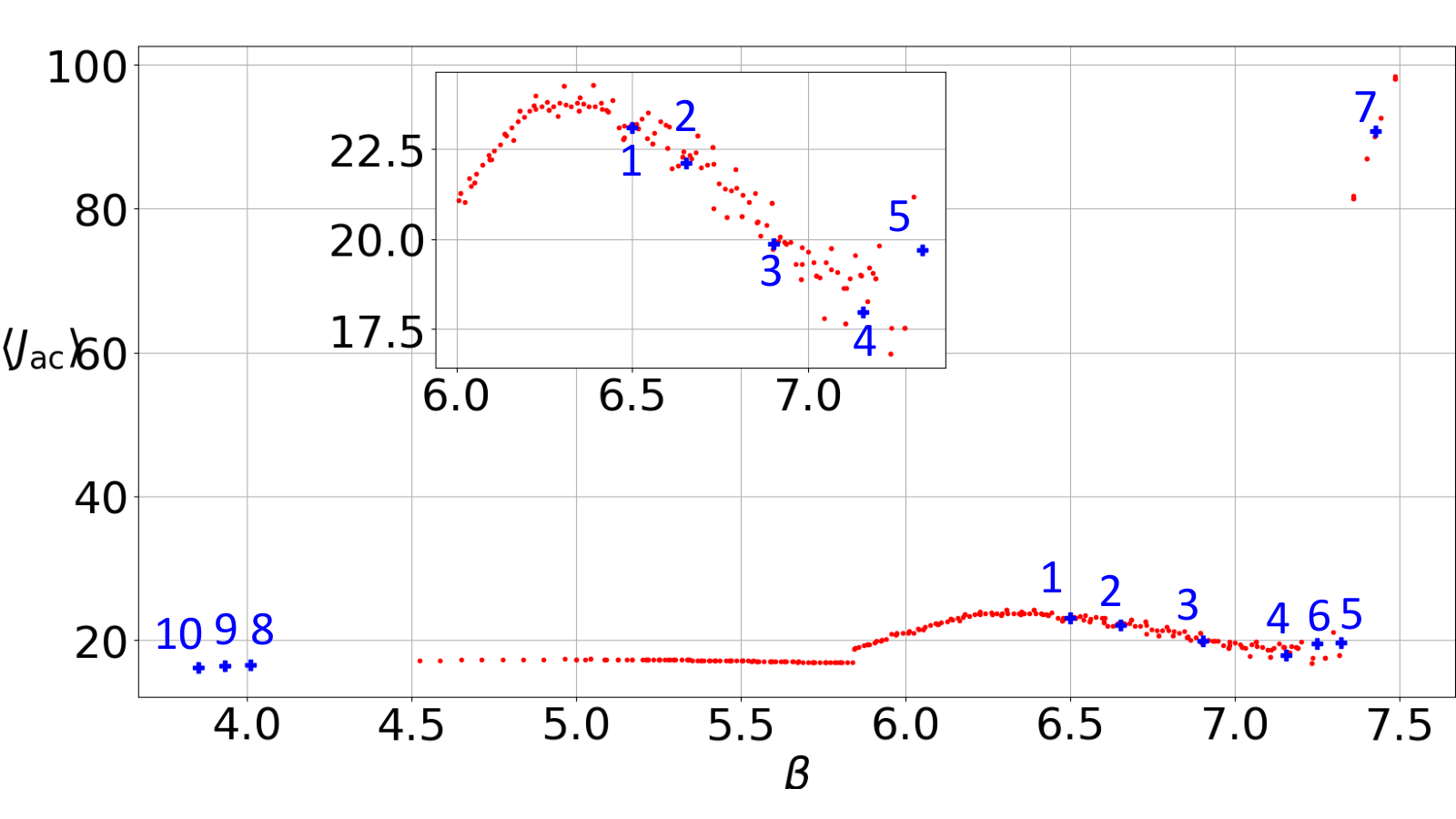
is met, where . This condition physically signifies that the optimization is successful when the system vibrates around the fixed point. In Figure 9, we show the optimization path (blue points) taken by this procedure, starting from We show the points numbered in the order in which they are encountered in the optimization procedure. As shown in the figure, the path leads to a reduction in by exiting the chaotic region into the periodic regions for larger of and eventually into the periodic region at smaller values of . We remark that, in this case, direct evaluation of the bifurcation diagram is possible, owing to the relatively low dimension of the system and the parameter space. This bifurcation diagram itself suggests optimal paths for acoustic energy reduction. However, in a more general setting, the dimension of the system, the objective function and parameter spaces may be such that bifurcation diagrams, at the resolution of parameters required to compute accurate gradients, are computationally infeasible. The demonstration in this section indicates that the shadowing sensitivities, which can be computed at a smaller cost relative to the bifurcation diagram computation, can be used instead, for optimization problems. For illustration purposes, we have chosen a simple gradient-descent with a fixed relaxation factor. The numerical results in Figure 9, however, show that the step size plays an important role in the rapid transition from large in the periodic region (around 7.4) to the periodic region for smaller values (around 4.0). We defer to a future work the effect of the step size, which is beyond the scope of this paper.
6 Data assimilation with discrete shadowing
A common problem whenever we have incomplete, and often noisy, observations together with a model of a physical system, is to estimate a model trajectory that reproduces the observations. In this section, we explain that the variational formulation of this problem is an application of the shadowing algorithm discussed in section 3. Then, we apply the shadowing algorithm to the time-delayed model to illustrate its potential for data assimilation in chaotic solutions.
In a data assimilation problem, we are given external measurements of an observable at a sequence of times, denoted . In the data assimilation method 4DVar [112], an initial state is sought so that the model trajectory at the observation times, produces a sequence that closely matches the observations . If a reliable guess for the initial state, known as background , is available, we desire our predicted initial state to be close to the background. The optimal initial state, known as analysis, is obtained by minimizing the following cost functional
| (48) |
The first term in the cost functional in Eq. 48 corresponds to the misfit between the predicted initial state and the background, where is a background error covariance matrix. The second term is the misfit between the external observations and values of the observable generated by the model, using the predicted state as the initial condition. Given an observable space of dimension , the matrix is the observation error covariance matrix. Without loss of generality, take and to be identity matrices (in and respectively), which results in the following cost functional:
| (49) |
The cost functional is minimized using a standard optimization procedure, and an analysis state is obtained. The reader is referred to [113] for data assimilation of nonchaotic states with a similar thermoacoustic model considered in the present paper. When the model is chaotic, the standard optimization procedure fails since the gradient of the functional with respect to grows exponentially with the time duration of available observations (Figure 1). Thus, assimilation for a time window longer than the typically short Lyapunov time, cannot be achieved using standard optimization methods.
However, several effective strategies have been proposed, particularly in the field of numerical weather prediction, wherein chaotic models are widely used, that are successful over long assimilation windows. The most popular of these include 4DVar-AUS, in which the analysis increment – the discrepancy added to the state during optimization – is restricted, to the nonstable () subspace, at every timestep [114]. Another method is projected shadowing-based data assimilation in which the cost functional is minimized using Newton’s method in each step of which the analysis trajectory, as a whole, is updated. Additionally, the updates to the analysis trajectory during each Newton iteration is carried out only on the nonstable subspace, and this leads to the economy of the method. The updates to the analysis trajectory on the stable subspace is treated using a different method, known as synchronization [115]. In this work, we present an alternative approach that uses the shadowing algorithm described in section 3. The goal of this approach is to compute a model orbit that shadows the pseudo-orbit pertaining to the observations. Our method thus joins the class of shadowing-based data assimilation methods offering an alternative formulation that indirectly computes the shadowing orbit through NILSS.
6.1 Tangent NILSS for state estimation with full-state observations
We introduced NILSS [36] as a method to differentiate long-time averages with respect to parameters in a chaotic system. How is the method relevant to the problem of state and parameter estimation? The answer to this question lies in the fact that a shadowing trajectory can be obtained as a byproduct of the NILSS method, and shadowing trajectories can be used for state estimation. First, we recognize that, in NILSS, the derivative of the long-time average is computed along a shadowing trajectory at a perturbed parameter. Secondly, we relate the shadowing perturbation sequence, , that is computed by tangent NILSS, to the solution of the state and parameter estimation problem.
6.1.1 Shadowing-based interpretation of NILSS
NILSS and its adjoint versions use the shadowing lemma (see e.g. 18.1.2 of [116]) by considering the reference trajectory as a pseudo-orbit of According to the shadowing lemma, there is a unique orbit of called the shadowing orbit, that is close to the given reference orbit of , . The tangent shadowing perturbation is the sequence of tangent vectors, along this shadowing orbit, that expresses the discrepancy between the shadowing orbit and the pseudo-orbit , in the limit Hence it remains bounded for all time. A close approximation of the shadowing perturbation, , is obtained by solving the following least squares problem ([38], Theorem LSS)
| (50) |
In the above optimization problem, the search space is restricted to a subset of in which each can be expressed as , i) for some , ii) where is the conventional tangent solution, i.e., solution of Eq. 3 with zero initial condition. This leads the NILSS algorithm [36] to being more efficient than if the search space was set to [36].
6.2 Converting the state estimation problem to a parameter estimation problem
The cost functional in state estimation consists of two parts: the background error and the observation error. We may assume that the background orbit is a pseudo-orbit of , for some around zero. Then, the shadowing problem (Eq. 50) minimizes the first part of the state estimation cost functional, which is the background error. In order to minimize the second part, the observation error, we use the observation error as the objective function in the shadowing algorithm. Through the parameter optimization procedure described in section 5, we find an optimal parameter that minimizes the observation error. This amounts to finding an such that the error between an observation orbit and a true orbit of is minimized. Then, we can refine the background trajectory, using the shadowing perturbation (computed by the shadowing algorithm). The parameter optimization is then repeated with the refined trajectory as the new background. By repeating this combined state-parameter optimization procedure, we minimize both parts of the state estimation cost functional separately. At the end of this procedure, the analysis state is obtained by iteratively refining the background state using the shadowing perturbations at different parameters. We outline the state-parameter optimization procedure assuming we have observations at every timestep. The following steps are repeated, until the cost functional is less than a specified tolerance. Initially, the reference orbit for shadowing is set to the background orbit. The algorithm is the following:
- 1.
- 2.
Update the parameter as: , where
- 3.
Update the initial condition for the next iteration as . Go to step 1.
In practice, the time corresponding to the start of the assimilation window, must be postponed roughly by (Lyapunov time), to allow a spin-up time for to be accurately computed.

The relaxation factor is assumed to be a fixed constant, as in the parameter optimization procedure in section 5.
6.3 Numerical results
We present state estimation results on the time-delayed model, computed using the above algorithm. The algorithm is validated on the Lorenz’63 model, as shown in Figure 12 in B. A total of 180 experiments are performed on the time-delayed model, each with a different background trajectory of length 20 time units. The parameter that is updated is set to with the reference value of 7.0. In each experiment, a background state is generated by perturbing each component of a reference state by a Gaussian random variable of variance 0.1. The original trajectory, started from the reference state, is used to generate the observations (of the acoustic energy) at every timestep. The mean squared observational error is the objective function for tangent NILSS,
The step size for gradient descent (section 5) is . We show in Figure 10 the relative errors in the acoustic energy along the analysis orbit, which is the result of the algorithm after 200 gradient descent steps. The relative error is defined as . Each colored line indicates a single experiment, with a total of 180 numerical experiments performed with different background states. The color of the line indicates the maximum relative error observed in that experiment, during the assimilation window of 20 units; the maximum errors increase from blue to green. The sample mean of the relative errors across all the experiments is shown in black. Note that the assimilation time is 4 times longer than the Lyapunov time. As shown in Figure 1, over 20 time units, we expect a small perturbation introduced in the initial condition, in almost any direction, to grow by 3 orders of magnitude. However, as the results in Figure 10 indicate, the relative error in has been restricted to within 10 % over this assimilation window, due to use of shadowing directions to iteratively refine the initial condition and the parameter, to match the observations. Improvements to this algorithm in order to reduce the errors, and further increase the predictability window will be studied in future work. One modification to the suggested algorithm, toward this goal, is to incorporate the observation error at every timestep, into the perturbation in the shadowing algorithm.
7 Conclusions
Naïve applications of linear perturbation methods such as tangent/adjoint/Automatic Differentiation (AD)/finite-difference, cannot compute the derivatives of long-time averages in chaotic systems with respect to specified inputs. A recent method, known as the Non-Intrusive Least Squares Shadowing [36], computes these derivatives by numerical construction of tangent/adjoint shadowing perturbations, which are infinitesimal perturbations that remain bounded for a long time duration. In this paper, we introduce AD into the tangent and adjoint NILSS. This nontrivial combination of algorithms is an enabler for the application of shadowing to complex dynamical systems. We demonstrate shadowing by computing sensitivities on a chaotic time-delayed model, which is a reduced-order model of a gas turbine combustor. We compute tangent and adjoint shadowing sensitivities of the ensemble averages of the acoustic energy and Rayleigh index with respect to the design parameters that control the heat release rate and the time delay. Although the model is a reduced representation compared to CFD-based combustion models, it can be used to estimate the development of chaotic acoustic instabilities. First, we demonstrate an automatically-differentiated procedure for the minimization of the long time-averaged acoustic energy through heat-release parameter selection, which does not require a tangent solver [33]. Secondly, we construct a pseudo-orbit data assimilation scheme using the computed shadowing sensitivities in an optimization loop. We show that this scheme extends the predictability window by four Lyapunov times. Finally, we remark that the proposed algorithm, the shadowing-based optimization and data assimilation scheme are more generally applicable. The algorithms and the software developed (available at [117]) may be used for other hyperbolic chaotic models with/without time delay.
Funding
Nisha Chandramoorthy and Qiqi Wang gratefully acknowledge the support of the Air Force Office of Scientific Research Grant No. FA8650-19-C-2207. Luca Magri gratefully acknowledges the support of the Royal Academy of Engineering Research Fellowships Scheme. Conflict of Interest: The authors declare that they have no conflict of interest.
Appendix A Validation of sensitivity computation on the Lorenz’63 model
We use the classical model of chaos, the Lorenz’63 system, for validation results in this paper. The Lorenz’63 model is the following set of nonlinear ODEs that serves as a reduced-order model for fluid thermal convection between parallel plates maintained at a temperature difference [118]:
| (52) |
Here a phase point is represented using 3 coordinates as and the map advances a state to by timestepping the ODE system (Eq. 52). For the time integration, we use a Forward Euler scheme with a timestep of 0.005. The Lyapunov exponents of this system are about 0.9, 0, and -14.6. This is a partially hyperbolic system [119] that has been shown to possess an SRB measure [120].
The objective function for validating shadowing is chosen to be the coordinate function. It is known that the
ergodic average as a function of , can be
approximated as a straight line with a slope of about 0.96, over a range of values around the standard [76]. We use the discrete shadowing algorithms described in section 3 in both tangent and adjoint mode, to compute this derivative. Numerical results are shown
in Figure 11, in which 100 sample sensitivities are shown each over a time duration of 15 units, starting from different points on the Lorenz’63 attractor. On the left, we see the computed tangent shadowing sensitivities with , and the on the right, the adjoint shadowing sensitivities, also computed with . From the numerical results, we see that the sample means of both sensitivities are within 10% of the reference value of 0.96, thus validating both tangent and adjoint shadowing sensitivity codes. These tests can be run from tests/test_lorenz63.jl at [117]. Interestingly, adjoint shadowing appears to be better suited for this objective function-parameter pair since the variance of tangent sensitivities is 10 times larger than the adjoint.


Appendix B Validation of data assimilation scheme on the Lorenz’63 model

We apply the data assimilation scheme described in section 6 on the Lorenz’63 model. We perform a series of 100 numerical experiments each with a different background. We fix a reference trajectory of length 5000 steps (10 time units), and generate a background by perturbing the reference initial condition in the direction by an additive Gaussian noise with a variance of 0.1. The reference trajectory is used to generate the observation trajectory Tangent NILSS is run with an objective function,
| (53) |
where is the -coordinate of a trajectory Using the derivative computed by shadowing, the parameter is updated in a gradient descent algorithm with a constant step size of . At the beginning of gradient descent, the trajectory is set to the background trajectory. At each gradient descent step, it is iteratively refined to a pseudo-orbit, as described in Step 3 in section 6. The mean error is calculated by averaging the optimal error across the 100 experiments. The optimal errors , defined as relative observation errors after 200 gradient descent steps, across experiments are as shown as a function of time in Figure 12. The relative observation error at time is . The colors of the lines in Figure 12 are according to the maximum over of the relative observation error. As mentioned before, the only positive Lyapunov exponent of this system is known to be about 0.9. The results indicate a predictability within 10% of the observation, on average, even up to 10 time units, which is about With this validation on the Lorenz’63 model, we apply the same method for data assimilation in the Rijke tube model, as described in section 6.
Appendix C AD shadowing and code for replication/extension
As we describe in the main text, the AD version of shadowing is enabled by the introduction of AD to replace the tangent/adjoint solvers in tangent/adjoint shadowing. In this section, we give a pseudocode for this modification. The source
code in Julia for generating the numerical results in this paper is available at [117]. This section also briefly describes how this code may be used with a different chaotic ODE/map.
We must mention that an alternative AD-version of the NILSS algorithm is also available at [121], in which the OpenAD AD software package [23, 25, 26], written in Fortran, is used. This latter code assumes that the primal solver is available from the user as a binary file.
In the AD version of tangent/adjoint shadowing, as mentioned before, we replace the needed tangent/adjoint solvers with AD. In order to do this, we define a function, say f, whose return value will be differentiated in forward/reverse-mode, and we specify some input variable(s) to differentiate with respect to. The AD software returns the gradient of the return value with respect to the input which is a function of the arguments passed to f. Let f be a function
with the arguments . The scalar or vector return value
of this function is written as .
For instance, using the Zygote.jl Julia package,
one would use the following syntax to obtain the gradient of with respect to :
. If using
the OpenAD Fortran package instead, we declare the
input and the output of f to be active variables. If ret_f is the variable that stores the return value of , its derivative with respect to is stored in the variable ret_f%d. In the AD version of tangent/adjoint shadowing, we only propose to modify the -loop in section 3.2 by introducing AD to replace the tangent/adjoint solvers; the rest of the algorithm is retained as described in section 3. The inputs to the AD shadowing algorithm are the sequences and . We now give the modified -loop in which we define the needed function, and input variables, for each AD invocation.
- 1.
Obtain from by applying AD. In particular,
- (a)
for tangent shadowing, we differentiate the function . The input variable is and the output is the return value of the function. The derivative obtained from forward-mode AD is , and this must be carried out for ;
- (b)
for adjoint shadowing, we differentiate the value , where . The input variable is . The derivative obtained from reverse-mode AD is , and this must be carried out for .
- (a)
- 2.
Let be the matrix with the columns , . QR-factorize and set to the obtained “Q”. Let the “R” from QR factorization be stored as . Thus, each , is now a unit vector.
- 3.
Obtain from by applying AD. In particular,
- (a)
for tangent shadowing, we differentiate the function . The input variable is . The derivative obtained from forward-mode AD is ;
- (b)
for adjoint shadowing, we differentiate the value . The input variable is . The derivative obtained from reverse-mode AD is .
- (a)
- 4.
Set , which is a -length orthogonal projection row-vector of along
- 5.
Normalize by projecting out the components along , that is, set
- 6.
Go to step 1 with , and repeat until
In the code at [117], the Julia script tests/test_lorenz63.jl and tests/test_rijke.jl compute respectively, for the Lorenz’63 model (Eq. 52) and the Rijke tube model (Eq. 33),
the tangent and adjoint shadowing sensitivities. In order to use the code
at [117] with a different model, we can use one of these test files as a template. The Julia file describing the model equations, which must be included in the test file, can follow the existing examples in examples/lorenz63.jl or examples/rijke.jl. The optimization and data assimilation routines described in section 5 and 6 respectively,
can also be applied to a new model. To do this, we include the file containing the
model equations into the utilities i) utils/optimize.jl for parameter optimization and
ii) utils/rijke_tangent_state_estimation.jl for the state estimation algorithm.
References
- [1] I. Sobol, S. Kucherenko, Derivative based global sensitivity measures and their link with global sensitivity indices, Mathematics and Computers in Simulation 79 (10) (2009) 3009–3017.
- [2] M. Lamboni, B. Iooss, A.-L. Popelin, F. Gamboa, Derivative-based global sensitivity measures: general links with sobol indices and numerical tests, Mathematics and Computers in Simulation 87 (2013) 45–54.
- [3] S. Ansuj, F. Shokooh, R. Schinzinger, Parameter estimation for induction machines based on sensitivity analysis, IEEE Transactions on Industry Applications 25 (6) (1989) 1035–1040.
- [4] S. Islam, D. Entekhabi, R. Bras, I. Rodriguez-Iturbe, Parameter estimation and sensitivity analysis for the modified bartlett-lewis rectangular pulses model of rainfall, Journal of Geophysical Research: Atmospheres 95 (D3) (1990) 2093–2100.
- [5] H. Agarwal, J. E. Renaud, E. L. Preston, D. Padmanabhan, Uncertainty quantification using evidence theory in multidisciplinary design optimization, Reliability Engineering & System Safety 85 (1) (2004) 281–294.
- [6] B. Lockwood, D. Mavriplis, Gradient-based methods for uncertainty quantification in hypersonic flows, Computers & Fluids 85 (2013) 27–38.
- [7] A. Sandu, D. N. Daescu, G. R. Carmichael, Direct and adjoint sensitivity analysis of chemical kinetic systems with kpp: Part i—theory and software tools, Atmospheric Environment 37 (36) (2003) 5083–5096.
- [8] R. H. Langland, N. L. Baker, Estimation of observation impact using the nrl atmospheric variational data assimilation adjoint system, Tellus A 56 (3) (2004) 189–201.
- [9] O. Talagrand, P. Courtier, Variational assimilation of meteorological observations with the adjoint vorticity equation. i: Theory, Quarterly Journal of the Royal Meteorological Society 113 (478) (1987) 1311–1328.
- [10] A. Saltelli, M. Ratto, T. Andres, F. Campolongo, J. Cariboni, D. Gatelli, M. Saisana, S. Tarantola, Global sensitivity analysis: the primer, John Wiley & Sons, 2008.
- [11] E. Borgonovo, E. Plischke, Sensitivity analysis: a review of recent advances, European Journal of Operational Research 248 (3) (2016) 869–887.
- [12] F. A. Viana, T. W. Simpson, V. Balabanov, V. Toropov, Special section on multidisciplinary design optimization: Metamodeling in multidisciplinary design optimization: How far have we really come?, AIAA Journal.
- [13] L. Magri, Adjoint Methods as Design Tools in Thermoacoustics, Applied Mechanics Reviews 71 (2) (2019) 020801. doi:10.1115/1.4042821.
- [14] M. Ghil, P. Malanotte-Rizzoli, Data assimilation in meteorology and oceanography, Advances in geophysics 33 (1991) 141–266.
- [15] P. Heimbach, V. Bugnion, Greenland ice-sheet volume sensitivity to basal, surface and initial conditions derived from an adjoint model, Annals of Glaciology 50 (52) (2009) 67–80.
- [16] J. Sobieszczanski-Sobieski, Sensitivity analysis and multidisciplinary optimization for aircraftdesign-recent advances and results, Journal of Aircraft 27 (12) (1990) 993–1001.
- [17] H. Kitano, Systems biology: a brief overview, Science 295 (5560) (2002) 1662–1664.
- [18] H. M. Bücker, G. Corliss, P. Hovland, U. Naumann, B. Norris, Automatic differentiation: applications, theory, and implementations, Vol. 50, Springer Science & Business Media, 2006.
- [19] A. Griewank, A. Walther, Evaluating derivatives: principles and techniques of algorithmic differentiation, SIAM, 2008.
- [20] A. Adcroft, J.-M. Campin, S. Dutkiewicz, C. Evangelinos, D. Ferreira, G. Forget, B. F.-K. P. Heimbach, C. Hill, E. Hill, H. Hill, O. Jahn, M. Losch, J. Marshall, G. Maze, D. Menemenlis, A. Molod, Mitgcm user manual, http://mitgcm.org/public/r2_manual/latest/ (2008).
- [21] C. Wunsch, P. Heimbach, R. M. Ponte, I. Fukumori, The global general circulation of the ocean estimated by the ecco-consortium, Oceanography 22 (2) (2009) 88–103.
- [22] P. Heimbach, D. Menemenlis, M. Losch, J.-M. Campin, C. Hill, On the formulation of sea-ice models. part 2: Lessons from multi-year adjoint sea-ice export sensitivities through the canadian arctic archipelago, Ocean Modelling 33 (1) (2010) 145–158.
- [23] J. Utke, U. Naumann, M. Fagan, N. Tallent, M. Strout, P. Heimbach, C. Hill, C. Wunsch, Openad/f: A modular open-source tool for automatic differentiation of fortran codes, ACM Transactions on Mathematical Software (TOMS) 34 (4) (2008) 18.
- [24] J. Utke, U. Naumann, Combinatorial problems in Open/AD, in: U. Naumann, O. Schenk (Eds.), Combinatorial Scientific Computing, Computational Science, Chapman and Hall/CRC, 2012, chap. 6.
- [25] M. Alexe, O. Roderick, M. Anitescu, J. Utke, T. Fanning, P. Hovland., Using automatic differentiation in sensitivity analysis of nuclear simulation models, Transactions of the American Nuclear Society 102 (2010) 235–237.
- [26] P. Hovland, B. Norris, M. Strout, S. Bhowmick, J. Utke, Sensitivity analysis and design optimiziation through automatic differentiation, in: A. M. et. al. (Ed.), SciDAC 2005, Vol. 16 of Journal of Physics: Conference Series, Bristol and Philadelphia publisher = Institute of Phsysics Publishing, 2005, pp. 466–470, online avaliable at http://www.iop.org/EJ/article/1742-6596/16/1/063/jpconf5_16_063.pdf.
- [27] L. Hascoët, M. Araya-Polo, The adjoint data-flow analyses: Formalization, properties, and applications, Lecture Notes in Computational Science and Engineering 50 (2006) 135.
- [28] L. Hascoet, V. Pascual, The tapenade automatic differentiation tool: principles, model, and specification, ACM Transactions on Mathematical Software (TOMS) 39 (3) (2013) 20.
- [29] P. J. Blonigan, P. Fernandez, S. M. Murman, Q. Wang, G. Rigas, L. Magri, Toward a chaotic adjoint for les, arXiv preprint arXiv:1702.06809.
- [30] V. Brunet, S. Deck, Zonal-detached eddy simulation of transonic buffet on a civil aircraft type configuration, NOTES ON NUMERICAL FLUID MECHANICS AND MULTIDISCIPLINARY DESIGN 97 (2008) 182.
- [31] A. Elmiligui, K. Abdol-Hamid, E. B. Parlette, Detached eddy simulation for the f-16xl aircraft configuration, in: 53rd AIAA Aerospace Sciences Meeting, 2015, pp. 2015–1496.
- [32] K. D. Squires, J. R. Forsythe, S. A. Morton, D. C. Blake, M. Serrano, K. E. Wurtzler, W. Z. Strang, R. F. Tomaro, P. Spalart, Analysis of full aircraft with massive separation using detached-eddy simulation, in: Proceedings of the High Performance Computing Modernization Program 2002 Users Group Conference, Austin, TX, June, 2002, pp. 9–14.
- [33]
F. Huhn, L. Magri, Stability,
sensitivity and optimisation of chaotic acoustic oscillations, Journal of
Fluid Mechanics 882 (2020) A24.
arXiv:1909.12979,
doi:10.1017/jfm.2019.828.
URL http://arxiv.org/abs/1909.12979 - [34]
F. Huhn, L. Magri, Optimisation of
chaotically perturbed acoustic limit cycles, Nonlinear 100 (2020)
1641–1657.
arXiv:1909.12979.
URL http://arxiv.org/abs/1909.12979 - [35] Q. Wang, Forward and adjoint sensitivity computation of chaotic dynamical systems, Journal of Computational Physics 235 (2013) 1–13.
- [36]
A. Ni, Q. Wang,
Sensitivity
analysis on chaotic dynamical systems by Non-Intrusive Least Squares
Shadowing (NILSS), Journal of Computational Physics 347 (2017) 56 – 77.
doi:https://doi.org/10.1016/j.jcp.2017.06.033.
URL http://www.sciencedirect.com/science/article/pii/S0021999117304783 - [37] A. Ni, Hyperbolicity, shadowing directions and sensitivity analysis of a turbulent three-dimensional flow, Journal of Fluid Mechanics 863 (2019) 644–669. doi:10.1017/jfm.2018.986.
- [38] Q. Wang, Convergence of the least squares shadowing method for computing derivative of ergodic averages, SIAM Journal on Numerical Analysis 52 (1) (2014) 156–170.
- [39] P. J. Blonigan, Adjoint sensitivity analysis of chaotic dynamical systems with non-intrusive least squares shadowing, Journal of Computational Physics 348 (2017) 803–826.
- [40] F. C. Cooper, P. H. Haynes, Climate sensitivity via a nonparametric fluctuation–dissipation theorem, Journal of the Atmospheric Sciences 68 (5) (2011) 937–953.
- [41] R. V. Abramov, A. J. Majda, Blended response algorithms for linear fluctuation-dissipation for complex nonlinear dynamical systems, Nonlinearity 20 (12) (2007) 2793.
- [42] M. Colangeli, V. Lucarini, Elements of a unified framework for response formulae, Journal of Statistical Mechanics: Theory and Experiment 2014 (1) (2014) P01002.
- [43] V. Lucarini, F. Ragone, F. Lunkeit, Predicting climate change using response theory: global averages and spatial patterns, Journal of Statistical Physics (2016) 1–29.
- [44] R. V. Abramov, A. J. Majda, New approximations and tests of linear fluctuation-response for chaotic nonlinear forced-dissipative dynamical systems, Journal of Nonlinear Science 18 (3) (2008) 303–341.
- [45] D. Ruelle, General linear response formula in statistical mechanics, and the fluctuation-dissipation theorem far from equilibrium, Physics Letters A 245 (3) (1998) 220–224.
- [46] Y. Kuang, Delay differential equations: with applications in population dynamics, Vol. 191, Academic Press, 1993.
- [47] H. L. Smith, An introduction to delay differential equations with applications to the life sciences, Vol. 57, Springer New York, 2011.
- [48] Y.-Y. Cao, P. M. Frank, Analysis and synthesis of nonlinear time-delay systems via fuzzy control approach, IEEE Transactions on fuzzy systems 8 (2) (2000) 200–211.
- [49] W. Zhang, M. S. Branicky, S. M. Phillips, Stability of networked control systems, IEEE Control Systems 21 (1) (2001) 84–99.
- [50] P. Baldi, A. F. Atiya, How delays affect neural dynamics and learning, IEEE Transactions on Neural Networks 5 (4) (1994) 612–621.
- [51] C. T. Baker, G. Bocharov, C. Paul, F. Rihan, Computational modelling with functional differential equations: Identification, selection, and sensitivity, Applied Numerical Mathematics 53 (2-4) (2005) 107–129.
- [52] S. Hussain, A. Basu, R. M. Wang, T. J. Hamilton, Delay learning architectures for memory and classification, Neurocomputing 138 (2014) 14–26.
- [53] T. C. Lieuwen, V. Yang, Combustion Instabilities in Gas Turbine Engines: Operational Experience, Fundamental Mechanisms, and Modeling, American Institute of Aeronautics and Astronautics, Inc., 2005.
- [54]
Lord Rayleigh,
The
explanation of certain acoustical phenomena, Nature 18 (1878) 319–321.
URL http://scholar.google.com/scholar?hl=en&btnG=Search&q=intitle:The+explanation+of+certain+acoustical+phenomena#0 - [55]
L. Kabiraj, R. I. Sujith, P. Wahi,
Bifurcations of Self-Excited
Ducted Laminar Premixed Flames, Journal of Engineering for Gas Turbines and
Power 134 (3) (2011) 31502.
doi:10.1115/1.4004402.
URL http://dx.doi.org/10.1115/1.4004402 - [56]
L. Magri, M. Bauerheim, F. Nicoud, M. P. Juniper,
Stability analysis of
thermo-acoustic nonlinear eigenproblems in annular combustors. Part II.
Uncertainty quantification, Journal of Computational Physics 325 (2016)
411–421.
arXiv:1602.08440,
doi:10.1016/j.jcp.2016.08.043.
URL http://dx.doi.org/10.1016/j.jcp.2016.08.043 - [57]
C. F. Silva, L. Magri, T. Runte, W. Polifke,
Uncertainty
Quantification of Growth Rates of Thermoacoustic Instability by an Adjoint
Helmholtz Solver, Journal of Engineering for Gas Turbines and Power 139 (1)
(2016) 011901.
doi:10.1115/1.4034203.
URL http://gasturbinespower.asmedigitalcollection.asme.org/article.aspx?doi=10.1115/1.4034203 - [58] G. A. Mensah, L. Magri, J. P. Moeck, Methods for the calculation of thermoacoustic stability margins and Monte-Carlo free uncertainty quantification, Journal of Engineering for Gas Turbines and Power 140 (6) (2018) 061501. doi:10.1115/1.4038156.
- [59]
N. Chandramoorthy, P. Fernandez, C. Talnikar, Q. Wang,
Feasibility analysis of ensemble
sensitivity computation in turbulent flows, AIAA Journal 57 (10) (2019)
4514–4526.
arXiv:https://doi.org/10.2514/1.J058127, doi:10.2514/1.J058127.
URL https://doi.org/10.2514/1.J058127 - [60] D. J. Lea, M. R. Allen, T. W. Haine, Sensitivity analysis of the climate of a chaotic system, Tellus A: Dynamic Meteorology and Oceanography 52 (5) (2000) 523–532.
- [61] G. L. Eyink, T. W. Haine, D. J. Lea, Ruelle’s linear response formula, ensemble adjoint schemes and Lévy flights, Nonlinearity 17 (5) (2004) 1867–1889. doi:10.1088/0951-7715/17/5/016.
- [62] V. Lucarini, F. Ragone, F. Lunkeit, Predicting climate change using response theory: Global averages and spatial patterns., J Stat Phys 166 (2017) 1036––1064. doi:10.1007/s10955-016-1506-z.
- [63] L. Young, What are srb measures, and which dynamical systems have them?., Journal of Statistical Physics 108 (2002) 733––754. doi:10.1023/A:1019762724717.
- [64]
G. Gallavotti, Entropy,
thermostats, and chaotic hypothesis, Chaos: An Interdisciplinary Journal of
Nonlinear Science 16 (4) (2006) 043114.
doi:10.1063/1.2372713.
URL http://aip.scitation.org/doi/10.1063/1.2372713 - [65] L. Arnold, H. Crauel, J.-P. Eckmann, Lyapunov Exponents, Lectures Notes in Mathematics 1486, Springer-Verlag, Berlin Heidelberg, 1990. doi:10.1007/978-3-540-78319-0.
- [66] C. Pugh, M. Shub, Stable ergodicity, Bulletin of the American Mathematical Society (N.S.) 41 (2004) 1–41. doi:10.1090/S0273-0979-03-00998-4.
- [67] P. V. Kuptsov, U. Parlitz, Theory and computation of covariant lyapunov vectors, Journal of Nonlinear Science 22 (2012) 727–762. arXiv:1105.5228, doi:10.1007/s00332-012-9126-5.
- [68]
A. Griewank, A. Walther,
Fundamentals
of Forward and Reverse, Society for Industrial and Applied Mathematics,
2008, Ch. 3, pp. 31–59.
arXiv:https://epubs.siam.org/doi/pdf/10.1137/1.9780898717761.ch3,
doi:10.1137/1.9780898717761.ch3.
URL https://epubs.siam.org/doi/abs/10.1137/1.9780898717761.ch3 - [69]
A. Griewank, A. Walther,
Jacobian
and Hessian Accumulation, Society for Industrial and Applied Mathematics,
2008, Ch. 10, pp. 211–243.
arXiv:https://epubs.siam.org/doi/pdf/10.1137/1.9780898717761.ch10,
doi:10.1137/1.9780898717761.ch10.
URL https://epubs.siam.org/doi/abs/10.1137/1.9780898717761.ch10 - [70]
A. Griewank, A. Walther,
Implicit
and Iterative Differentiation, Society for Industrial and Applied
Mathematics, 2008, Ch. 15, pp. 367–396.
arXiv:https://epubs.siam.org/doi/pdf/10.1137/1.9780898717761.ch15,
doi:10.1137/1.9780898717761.ch15.
URL https://epubs.siam.org/doi/abs/10.1137/1.9780898717761.ch15 - [71] M. Innes, Don’t Unroll Adjoint: Differentiating SSA-Form Programs, arXiv e-prints (2018) arXiv:1810.07951arXiv:1810.07951.
- [72]
autodiff.org, Tools for automatic
differentiation (2020).
URL http://www.autodiff.org/?module=Tools - [73] M. Innes, A. Edelman, K. Fischer, C. Rackauckas, E. Saba, V. B. Shah, W. Tebbutt, A differentiable programming system to bridge machine learning and scientific computing, ArXiv abs/1907.07587.
- [74] C. Rackauckas, Y. Ma, V. Dixit, X. Guo, M. Innes, J. Revels, J. Nyberg, V. D. Ivaturi, A comparison of automatic differentiation and continuous sensitivity analysis for derivatives of differential equation solutions, ArXiv abs/1812.01892.
- [75] J. Hückelheim, N. Kukreja, S. Narayanan, F. Luporini, G. Gorman, P. Hovland, Automatic differentiation for adjoint stencil loops, Proceedings of the 48th International Conference on Parallel Processing.
- [76] D. J. Lea, M. R. Allen, T. W. N. Haine, Sensitivity analysis of the climate of a chaotic system, Tellus Series a-Dynamic Meteorology and Oceanography 52 (5) (2000) 523–532. doi:10.1256/qj.01.180.
- [77] F. Ginelli, P. Poggi, A. Turchi, H. Chaté, R. Livi, A. Politi, Characterizing dynamics with covariant lyapunov vectors, Physical Review Letters 99 (13) (2007) 130601. arXiv:0706.0510, doi:10.1103/PhysRevLett.99.130601.
- [78] A. Ni, Adjoint shadowing directions in hyperbolic systems for sensitivity analysis (2018). arXiv:1807.05568.
- [79]
A. Ni, C. Talnikar,
Adjoint
sensitivity analysis on chaotic dynamical systems by Non-Intrusive
Least Squares Adjoint Shadowing (NILSAS), Journal of Computational
Physics 395 (2019) 690–709.
doi:10.1016/j.jcp.2019.06.035.
URL http://www.sciencedirect.com/science/article/pii/S0021999119304437 - [80] A. Ni, Approximating Ruelle’s linear response formula by shadowing methods, arXiv e-prints (2020) arXiv:2003.09801arXiv:2003.09801.
- [81] N. Chandramoorthy, Q. Wang, A computable realization of Ruelle’s formula for linear response of statistics in chaotic systems, arXiv e-prints (2020) arXiv:2002.04117arXiv:2002.04117.
- [82] A. A. Sliwiak, N. Chandramoorthy, Q. Wang, Ergodic Sensitivity Analysis of One-Dimensional Chaotic Maps, arXiv e-prints (2020) arXiv:2007.15594arXiv:2007.15594.
- [83]
R. V. Abramov, A. J. Majda,
Blended response
algorithms for linear fluctuation-dissipation for complex nonlinear dynamical
systems, Nonlinearity 20 (12) (2007) 2793–2821.
doi:10.1088/0951-7715/20/12/004.
URL https://doi.org/10.1088%2F0951-7715%2F20%2F12%2F004 - [84] C. H. Bischof, P. D. Hovland, B. Norris, On the implementation of automatic differentiation tools, Higher-Order and Symbolic Computation 21 (3) (2008) 311–331. doi:10.1007/s10990-008-9034-4.
- [85]
J. Hückelheim, P. Hovland, M. Strout, J.-D. Müller,
Parallelizable adjoint
stencil computations using transposed forward-mode algorithmic
differentiation, Optimization Methods and Software 33 (4-6) (2018) 672–693.
arXiv:https://doi.org/10.1080/10556788.2018.1435654, doi:10.1080/10556788.2018.1435654.
URL https://doi.org/10.1080/10556788.2018.1435654 - [86]
A. P. Dowling,
Nonlinear
self-excited oscillations of a ducted flame, Journal of Fluid Mechanics 346
(1997) 271–290.
doi:10.1017/S0022112097006484.
URL http://www.journals.cambridge.org/abstract_S0022112097006484 - [87]
A. P. Dowling,
A
kinematic model of a ducted flame, Journal of Fluid Mechanics 394 (1999)
51–72.
doi:10.1017/S0022112099005686.
URL http://www.journals.cambridge.org/abstract_S0022112099005686 - [88]
H. Gotoda, H. Nikimoto, T. Miyano, S. Tachibana,
Dynamic properties of
combustion instability in a lean premixed gas-turbine combustor., Chaos
21 (1) (2011) 013124.
doi:10.1063/1.3563577.
URL http://www.ncbi.nlm.nih.gov/pubmed/21456838 - [89]
H. Gotoda, T. Ikawa, K. Maki, T. Miyano,
Short-term prediction of
dynamical behavior of flame front instability induced by radiative heat
loss., Chaos 22 (1) (2012) 033106.
doi:10.1063/1.4731267.
URL http://www.ncbi.nlm.nih.gov/pubmed/23020445 - [90] L. Kabiraj, A. Saurabh, P. Wahi, R. I. Sujith, Route to chaos for combustion instability in ducted laminar premixed flames, Chaos 22 (2) (2012) 0–12. doi:10.1063/1.4718725.
- [91]
I. C. Waugh, K. Kashinath, M. P. Juniper,
Matrix-free
continuation of limit cycles and their bifurcations for a ducted premixed
flame, Journal of Fluid Mechanics 759 (2014) 1–27.
doi:10.1017/jfm.2014.549.
URL http://www.journals.cambridge.org/abstract_S0022112014005497 - [92]
K. Kashinath, I. C. Waugh, M. P. Juniper,
Nonlinear
self-excited thermoacoustic oscillations of a ducted premixed flame:
bifurcations and routes to chaos, Journal of Fluid Mechanics 761 (2014)
399–430.
doi:10.1017/jfm.2014.601.
URL http://www.journals.cambridge.org/abstract_S0022112014006016 - [93]
a. Orchini, S. J. Illingworth, M. P. Juniper,
Frequency
domain and time domain analysis of thermoacoustic oscillations with
wave-based acoustics, Journal of Fluid Mechanics 775 (2015) 387–414.
doi:10.1017/jfm.2015.139.
URL http://www.journals.cambridge.org/abstract_S0022112015001391 - [94] V. Nair, G. Thampi, R. I. Sujith, Intermittency route to thermoacoustic instability in turbulent combustors, Journal of Fluid Mechanics 756 (2014) 470–487. doi:10.1017/jfm.2014.468.
- [95]
V. Nair, R. I. Sujith,
A
reduced-order model for the onset of combustion instability: Physical
mechanisms for intermittency and precursors, Proceedings of the Combustion
Institute, in press 35 (3) (2015) 3193–3200.
doi:10.1016/j.proci.2014.07.007.
URL http://linkinghub.elsevier.com/retrieve/pii/S1540748914003174 - [96] J.-P. Eckmann, Roads to turbulence in dissipative dynamical systems, Reviews of Modern Physics 53 (4) (1981) 643–654.
- [97] J. Miles, Strange attractors in fluid dynamics, Advances in Applied Mechanics 24 (1984) 189–214.
- [98] J. P. Eckmann, D. Ruelle, Ergodic theory of chaos and strange attractors, Reviews of Modern Physics 57 (1985) 617–656. doi:10.1103/RevModPhys.57.617.
- [99] P. Subramanian, R. Sujith, P. Wahi, Subcritical bifurcation and bistability in thermoacoustic systems, Journal of Fluid Mechanics 715 (2013) 210–238.
- [100] L. D. Landau, On the problem of turbulence, Dokl. Akad. Nauk SSSR 44 (8) (1944) 339–349.
- [101] L. D. Landau, E. M. Lifshitz, Fluid Mechanics, 2nd Edition, Pergamon Press, 1987.
- [102] T. Lieuwen, Dynamics of Harmonically Excited Flames.
- [103] L. Magri, M. P. Juniper, Sensitivity analysis of a time-delayed thermo-acoustic system via an adjoint-based approach, Journal of Fluid Mechanics 719 (2013) 183–202. doi:10.1017/jfm.2012.639.
- [104] L. N. Trefethen, M. Embree, Spectra and Pseudospectra, Princeton University Press, 2005.
- [105] C. Rackauckas, Q. Nie, Differentialequations. jl–a performant and feature-rich ecosystem for solving differential equations in julia, Journal of Open Research Software 5 (1).
- [106] C. Rackauckas, M. Innes, Y. Ma, J. Bettencourt, L. White, V. Dixit, Diffeqflux. jl-a julia library for neural differential equations, arXiv preprint arXiv:1902.02376.
- [107] L. Magri, M. P. Juniper, J. P. Moeck, Sensitivity of the rayleigh criterion in thermoacoustics, Journal of Fluid Mechanics 882 (2020) R1. doi:10.1017/jfm.2019.860.
- [108] B. T. Chu, On the Energy Transfer to Small Disturbances in Fluid Flow (Part I), Acta Mechanica 1 (3) (1965) 215–234.
- [109]
K. J. George, R. Sujith,
Disturbance
energy norms: A critical analysis, Journal of Sound and Vibration 331 (7)
(2012) 1552–1566.
doi:10.1016/j.jsv.2011.11.027.
URL http://linkinghub.elsevier.com/retrieve/pii/S0022460X11009059 - [110] L. Magri, Adjoint methods in thermo-acoustic and combustion instability, Ph.D. thesis, University of Cambridge (2015).
- [111]
R. S. Blumenthal, A. K. Tangirala, R. Sujith, W. Polifke,
A systems
perspective on non-normality in low-order thermoacoustic models: Full norms,
semi-norms and transient growth, International Journal of Spray and
Combustion Dynamics 9 (1) (2016) 19–43.
doi:10.1177/1756827716652474.
URL http://scd.sagepub.com/lookup/doi/10.1177/1756827716652474 - [112] T. Traverso, A. Bottaro, L. Magri, Data assimilation in thermoacoustic instability with Lagrangian optimization, EuroMech Vienna.
- [113] T. Traverso, L. Magri, Data Assimilation in a Nonlinear Time-Delayed Dynamical System with Lagrangian Optimization, in: Lecture Notes in Computer Science (including subseries Lecture Notes in Artificial Intelligence and Lecture Notes in Bioinformatics), Vol. 11539 LNCS, Springer, 2019, pp. 156–168. doi:10.1007/978-3-030-22747.
- [114]
A. Trevisan, M. D’Isidoro, O. Talagrand,
Four-dimensional
variational assimilation in the unstable subspace (4DVar-AUS) and the optimal
subspace dimension, Quarterly Journal of the Royal … 133 (October)
(2007) 937–948.
arXiv:arXiv:0801.1618v2, doi:10.1002/qj.
URL http://onlinelibrary.wiley.com/doi/10.1002/qj.71/abstract - [115]
B. de Leeuw, S. Dubinkina, J. Frank, A. Steyer, X. Tu, E. V. Vleck,
Projected
Shadowing-Based Data Assimilation, SIAM J. Appl. Dyn. Syst. 17 (4)
(2018) 2446–2477.
doi:10.1137/17M1141163.
URL https://epubs.siam.org/doi/10.1137/17M1141163 - [116] A. Katok, B. Hasselblatt, Introduction to the modern theory of dynamical systems, Vol. 54, Cambridge university press, 1997.
- [117]
N. Chandramoorthy,
nishaChandramoorthy/energies:
Thermoacoustics paper (Aug. 2020).
doi:10.5281/zenodo.3996268.
URL https://doi.org/10.5281/zenodo.3996268 - [118] E. N. Lorenz, Deterministic nonperiodic flow, Journal of the atmospheric sciences 20 (2) (1963) 130–141.
- [119]
V. Araújo, I. Melbourne, P. Varandas,
Rapid Mixing for
the Lorenz Attractor and Statistical Limit Laws for Their
Time-1 Maps, Commun. Math. Phys. 340 (3) (2015) 901–938.
doi:10.1007/s00220-015-2471-0.
URL http://link.springer.com/10.1007/s00220-015-2471-0 - [120] M. Holland, I. Melbourne, Central limit theorems and invariance principles for lorenz attractors, Journal of the London Mathematical Society 76 (2007) 345–364. doi:10.1112/jlms/jdm060.
- [121] N. Chandramoorthy, S. H. K. Narayanan, Q. Wang, P. Hovland, Tangent and adjoint ad-nilss, https://github.com/nishachandramoorthy/fds (2017).