Experimental lower bounds to the classical capacity of quantum channels

The complete characterization of quantum channels by quantum process tomography nielsen97; pcz; mls; dlp; qht; alt; cnot; ion; mohseni; irene; atom is demanding in terms of state preparation and/or measurement settings, since for increasing dimension $d$ of the system Hilbert space it scales as $d^{4}$. When one is interested in certifying specific properties of a quantum channels, more affordable procedures can be devised without resorting to complete quantum process tomography. This is the case of the detection of entanglement-breaking properties qchanndet; qchanndet2 or non-Markovianity nomadet of quantum channels, or the certification of lower bounds to the quantum capacity of noisy quantum channels ms16; ms-corr; exp; correxp. Typically, these direct methods have also the advantage of being more precise with respect to complete process tomography, which has the drawback of involving larger statistical errors due to error propagation.

One of the most relevant property of quantum channels is the classical capacity hol0; sw; hol for its operational importance in the quantification of the classical information that can be reliably transmitted. For the purpose of detecting lower bounds to the classical capacity, an efficient and versatile procedure has been recently proposed in Ref. ms19. The method allows to experimentally detect lower bounds to the classical capacity of completely unknown quantum channels just by means of few local measurements, even for high-dimensional systems multi.

The gist of the procedure is to efficiently reconstruct a number of probability transition matrices for suitable input states (playing the role of “encoding”) and matched output projective measurements (the corresponding “decoding”). The method is accompanied by the optimization of the prior distribution for the single-letter encoding pertaining to each input/output transition matrix. In this way, the mutual information for different communication settings is recovered and the resulting values are compared. Hence, a lower bound to the Holevo capacity and then a certification of the minimum reliable transmission capacity is achieved. Similarly to the method of certification for the quantum capacity ms16; ms-corr; exp, here each of the conditional probabilities corresponding to a communication setting can be obtained by preparing just an initial fixed bipartite state, where only one party enters the quantum channel, while local measurements are performed at the input and output of the channel.

In this paper we present an experimental demonstration for the above certification of classical capacity in noisy qubit channels. We implement the method by using highly-pure polarization entangled photons pairs, where the encoding/decoding settings are achieved by exploiting complementary observables of the polarization state. Moreover, a faithful deconvolution of noise is performed over the experimental data, which allows to optimize the reconstruction of the probability transition matrices.

Let us briefly review the method proposed in Ref. ms19 for bounding from below the classical capacity, with specific attention to the case of single-qubit quantum channels.

The classical capacity $C$ of a noisy quantum channel ${\cal E}$ quantifies the maximum number of bits that can be reliably transmitted per channel use, and it is given by the regularized expression hol0; sw; hol $C=\lim_{N\rightarrow\infty}\chi({\cal E}^{\otimes N})/N$, with $N$ as the number of uses, in terms of the Holevo capacity

where $S(\rho)=-\mathrm{Tr}[\rho\log_{2}\rho]$ denotes the Von Neumann entropy. The Holevo capacity $\chi({\cal E})\equiv C_{1}$, also known as one-shot classical capacity, is a lower bound for the ultimate channel capacity $C$, and also an upper bound for the mutual information mutu; mutu2; mutu3

where any transition matrix $Q(y|x)$ corresponds to the conditional probability for outcome $y$ in an arbitrary measurement at the output of a single use of the channel with input $\rho_{x}$, and $p_{x}$ denotes an arbitrary prior probability, which corresponds to the distribution of the encoded alphabet on the quantum states $\{\rho_{x}\}$.

As depicted in Fig. 1, in order to obtain a witness for the classical capacity without resorting to complete process tomography one can proceed as follows. Prepare a bipartite maximally entangled state $|\phi^{+}\rangle=\frac{1}{\sqrt{d}}\sum_{k=0}^{d-1}|k_{s}\rangle|k_{a}\rangle$ between a system and ancillary spaces, both with dimension $d$; send $|\phi^{+}\rangle$ through the unknown channel by keeping the action of ${\cal E}$ on the system alone, namely via the map ${\cal E}\otimes\mathbb{I}_{a}$; finally, measure locally a number of observables of the form $X_{\alpha}\otimes X_{\alpha}^{\tau}$, where $\tau$ denotes the transposition w.r.t. to the fixed basis defined by $|\phi^{+}\rangle$.

In fact, by denoting the $d$ eigenvectors of $X_{\alpha}$ as $\{|\phi^{(\alpha)}_{i}\rangle\}$, from the identity pla

with arbitrary operators $A$ and $B$, the detection scheme allows to reconstruct the set of conditional probabilities

For each encoding-decoding scheme $\alpha$ characterized by the choice of $X_{\alpha}$, we can write the corresponding optimal mutual information, namely the Shannon capacity

Then, we have the chain of inequalities

where $C_{D}$ is the experimentally accessible witness that depends on the chosen set of measured observables labeled by $\alpha$, and provides a lower bound to the classical capacity of the unknown channel.

In the present scenario we consider single-qubit channels and the information settings correspond to the choice of the three local observables $\sigma_{x}\otimes\sigma_{x}$, $\sigma_{y}\otimes\sigma_{y}$ and $\sigma_{z}\otimes\sigma_{z}$. Hence, each of the three conditional probabilities $Q^{(\alpha)}(j|i)$, with $\alpha=x,y,z$, is a $2\times 2$ transition matrix that corresponds to a binary classical channel, for which the optimal prior probability $\{p_{i}^{(\alpha)}\}$ can be theoretically evaluated ms19. In fact, without loss of generality, for each transition matrix we can fix the labeling of logical zeros and ones such that $0\leq\epsilon_{0}\leq\frac{1}{2}$, $\epsilon_{0}\leq\epsilon_{1}$, and $\epsilon_{0}\leq 1-\epsilon_{1}$, where $\epsilon_{0}$ denotes the error probability of receiving $1$ for input $0$, and $\epsilon_{1}$ denotes the error probability of receiving $0$ for input $1$. Then, for each $\alpha=x,y,z$ the mutual information as in Eq. (5) is maximized by a prior probability $\{p_{0},p_{1}=1-p_{0}\}$, with

where $z=2^{\frac{H[\epsilon_{0}]-H[\epsilon_{1}]}{1-\epsilon_{0}-\epsilon_{1}}}$, and $H(p)=-p\log_{2}p-(1-p)\log_{2}(1-p)$ denotes the binary Shannon entropy. The corresponding capacity is given by ms19

Notice that for $\epsilon_{0}=\epsilon_{1}=\epsilon$ one recovers the classical capacity for the binary symmetric channel

with uniform optimal prior $\{1/2,1/2\}$, whereas for $\epsilon_{0}=0$ (i.e., when only input 1 is affected by error) one obtains the capacity of the so-called $Z$-channel

In Appendix A we summarize the expected theoretical results for the qubit channels that we implemented experimentally.

In order to consider the experimental imperfections in our state preparation, we assume a Werner form

where $F=\braket{\Phi^{+}|\rho_{F}|\Phi^{+}}$ denotes the fidelity with respect to the ideal maximally entangled state $\ket{\Phi^{+}}=\frac{1}{\sqrt{2}}\left(\ket{0}\ket{0}+\ket{1}\ket{1}\right)$. Hence, we can replace Eq. (3) with

Equation (12) allows one to deconvolve the noise as long as $F\neq 1/4$, since the output state $({\cal E}\otimes\mathbb{I}_{a})\rho_{F}$ faithfully represents the unknown channel ${\cal E}$.

The normalized conditional probabilities for the three binary classical channels corresponding to the information settings $\alpha=x,y,z$ where coding and decoding are performed using the eigenstates of the three Pauli matrices $\sigma_{x},\sigma_{y},\sigma_{z}$ can be obtained by the ratio $\frac{\mathrm{Tr}[A{\cal E}(B)]}{\mathrm{Tr}[{\cal E}(B)]}$, when replacing $A$ and $B$ with the pertaining eigenvectors. In practical terms, these quantities are measured from the bipartite qubit detections, which in optical channels corresponds to two-photon coincidence detections $C(ji)=\mathrm{Tr}[(|j\rangle\langle j|_{S}\otimes|i\rangle\langle i|_{A})({\cal E}\otimes\mathbb{I}_{a})\rho_{F}]$ on the output state. We provide in Appendix B the explicit expressions for the conditional probabilities in terms of the measured coincidences. For each information setting $\alpha=x,y,z$, the logical bits and their pertaining transition error probabilities $\epsilon^{(\alpha)}_{0}$ and $\epsilon^{(\alpha)}_{1}$ introduced before Eq. (7) are identified from the conditional probabilities as follows

Using Eq. (8), from the experimental data we then obtain $C^{(\alpha)}=C_{B}(\epsilon^{(\alpha)}_{0},\epsilon^{(\alpha)}_{1})$, and hence the detected classical capacity as

We remark that the effect of a fidelity value $F<1$ (except the case $F=\frac{1}{4}$) is not detrimental for accessing the capacity witness $C_{D}$, and only the statistical noise is expected to increase for decreasing value of $F$. This can be argued from the identity (12) which, for any couple of bases $\{|i\rangle_{A}\}_{i=0,1}$ and $\{|j\rangle_{S}\}_{j=0,1}$, provides an unbiased estimation of the joint probabilities $p_{F}(j,i)=\mathrm{Tr}[(|j\rangle\langle j|_{S}\otimes|i\rangle\langle i|_{A})({\cal E}\otimes\mathbb{I}_{a})\rho_{F}]$ pertaining to the case of ideal fidelity $F=1$ in terms of the measured probabilities as

By denoting with $\sigma$ the typical order of magnitude of the standard deviation for the measured joint probabilities with $F<1$, then the noise deconvolution provides the correct probabilities with standard deviation

A single-mode continuous-wave laser at 405nm was used to pump a Type-II ppKTP crystal within a Sagnac interferometer (SI) in order to produce polarization-entangled photon pairs at 810nm via spontaneous parametric down conversion, as implemented in exp. The two output modes were labeled as $s$-qubit and $a$-qubit, so the Bell state $\ket{\Phi^{+}}=\frac{1}{\sqrt{2}}\left(\ket{H_{s}}\ket{H_{a}}+\ket{V_{s}}\ket{V_{a}}\right)$ was generated. As shown in the full scheme of Fig. 2, tube lenses with $F_{1}=300mm$ collimate both output modes, while objective lenses with $F_{2}=11mm$ couple them into single-mode-fibers (SMFs).

The fidelity of the experimental state $\rho_{F}$ defined in Eq. (11) and measured by quantum tomography techniques tomo1; tomo2 was $F=\braket{\Phi^{+}|\rho_{F}|\Phi^{+}}=0.979\pm 0.011$. Hence, we use Eq. (12) for noise deconvolution, and the standard deviation of the joint probabilities are increased just by $1.45\%$ with respect to the ideal case $F=1$, according to Eq. (16).

The observables $\sigma_{\alpha}$, for $\alpha=x,y,z$, are measured with rotations of a quarter wave-plate (QWP) and a half wave-plate (HWP) before a polarizing beam splitter (PBS) for each qubit. Remaining photon pairs after these projections are measured with synchronized single-photon avalanche detectors (SPADs) within a time window of 5ns for an integration time of 10s/measurement.

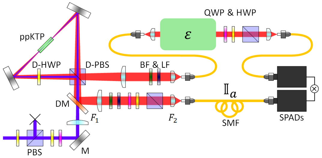
By referring to the parametrization of channels given in Appendix A, within the family of Pauli channels we have chosen two special cases as implemented in exp; pc. The first one is the phase damping (PD) channel (described by $q_{z}=q$ and $q_{x}=q_{y}=0$ in Appendix A). The second one is the depolarizing (D) channel (described by $q_{x}=q_{y}=q_{z}=q$). Their experimental simulations were implemented by $q_{i}$-weighted combinations of independent Pauli operations, achieved by setting a HWP at $0^{\circ}$-degrees ($45^{\circ}$-degrees) for $\sigma_{z}$ ($\sigma_{x}$) and a liquid crystal (LC) at minimum (maximum) voltage for $\sigma_{z}$ ($\mathbb{I}$) [see Fig. 2b]. Accordingly, the simultaneous operation $\sigma_{y}=i\sigma_{x}\sigma_{z}$ give us the last Pauli operation.

The experimental simulation of an amplitude damping (AD) channel was achieved by using a square SI with displaced trajectories as implemented in exp; adc2, where a HWP at $0^{\circ}$-degrees was placed in the H-polarized counter-clockwise trajectory, while another HWP at $\omega=\frac{\arccos(-\sqrt{1-\eta})}{2}$ degrees was place in the V-polarized clock-wise trajectory. The induced rotation of a single polarization (or damping) sends this light to the long arm of an unbalanced Mach-Zehnder interferometer (MZI), which then re-combines it out of coherence in a non-polarizing beam splitter (BS).

In Fig. 3 we show the measured Shannon capacities $C^{(\alpha)}$ in all three bases for the experimental simulation of three different environments, namely a PD-channel, a D-channel, and an AD-channel. This is compared to the predicted behaviour for the real input state, which is fidelity-dependent from Eq. (12) and in detail explained in the Appendix B. See Appendix C for details on the noise propagation and Appendix D for details on the experimental raw data.

For a PD-channel the witness $C_{D}$ of the channel capacity is obtained for $\alpha=z$ and can be compared with the expected theoretical value $C_{D}=1$. The presented results confirm the behavior in which phase-damping processes do not affect binary data transmission in the logical basis, but only in complementary superposition bases. The systematic offset below unity value is due to the propagation of error by replacing experimental negative values of $\epsilon_{0}^{(z)}$ with their absolute values. We observe that the customary constrained maximum-likelihood technique can solve the possible issue of negative reconstructed probabilities and the resulting bias in the capacity bounds.

For a D-channel the theoretical value $C_{D}=1-H(2q)$ is equally achieved by any of the three bases. Here, we find the best agreement with respect to this prediction, because small differences of the experimental state or channel from the ideal ones are rapidly compensated during the decoherence process by the simultaneous action of all three Pauli operations. Accordingly, the balance increase (decrease) in the diagonal (off-diagonal) terms of the density matrix reduces bias projections and final data dispersion.

For an AD-channel the experimental implementation requires control on multiple optical paths, where systematic error can have unbalanced contribution among different bases. Such an issue, combined with the non-linear dependency of $\eta$ with respect to $\omega$ and an angular uncertainty of $0.5^{\circ}$-degrees, gives considerable propagated errors. The expected capacity witness $C_{D}=1-H\left(\frac{1-\sqrt{1-\eta}}{2}\right)$ is achieved equivalently by the bases $x$ or $y$. Our method still succeeds in showing the general behavior and providing a sensible lower bound to the classical channel capacity.

In summary, by comparison with the theoretical predictions, the method proved to be very effective in providing a witness for the classical capacity of noisy quantum channels, even if the channel implementation has critical and systematic imperfections. Moreover, by means of the noise deconvolution, we have shown that the method is robust with respect to an imperfect probe-state preparation and provides an unbiased estimation of the theoretical lower bounds.

The experimental coincidence counts allow to directly reconstruct the sets of conditional probabilities for three different information settings. For each setting $\alpha=x,y,z$, by Eq. (13) the logical bits and the values of $\epsilon_{0}^{(\alpha)}$ and $\epsilon_{1}^{(\alpha)}$ are identified. From these values one recovers three values of $C_{B}$ as in Eq. (8), which correspond to the Shannon capacity, namely the optimized mutual information for coding/decoding on the eigenstates of $\sigma_{x}$, $\sigma_{y}$, and $\sigma_{z}$. The highest among such three values is selected as a classical capacity witness, namely it certifies a lower bound to the ultimate classical capacity of the unknown quantum channel. For each information setting, by Eq. (7) the identified values of $\epsilon_{0}^{(\alpha)}$ and $\epsilon_{1}^{(\alpha)}$ also allow one to obtain the optimal weight for the coding of the two logical characters.

We emphasize that our method is highly robust against experimental imperfections, even in cases where the prepared quantum state is partially mixed as the Werner state. For each of the three chosen bases, the Shannon capacity is precisely retrieved for all values of the channel parameters. Nevertheless, the most accurate values were obtained for the Pauli channels, which are effectively produced by mixing unitary operations over the input state. For mixtures of non-unitary operations as the amplitude damping channel, we find a less smooth behavior in the detected classical capacity because experimental imperfections do not act in balanced ways for both photon polarizations.

We recommend this novel method for certifying the classical capacity of quantum channels due to its high precision under different scenarios. The studied cases were not particularly designed to match with the protocol, but chosen to represent a variety of classes. No prior information is needed about the channel structure, while the measurement settings are much less demanding with respect to full process tomography.

References

- (1) I. L. Chuang and M. A. Nielsen, J. Mod. Optics 44, 2455 (1997).
- (2) J. F. Poyatos, J. I. Cirac, and P. Zoller, Phys. Rev. Lett. 78, 390 (1997).
- (3) M. F. Sacchi, Phys. Rev. A 63, 054104 (2001).
- (4) G. M. D’Ariano and P. Lo Presti, Phys. Rev. Lett. 86, 4195 (2001).
- (5) G. M. D’Ariano, M. G. A. Paris, and M. F. Sacchi, Quantum Tomography, Advances in Imaging and Electron Physics 128, p. 205-308 (2003).
- (6) J. B. Altepeter, D. Branning, E. Jeffrey, T. C. Wei, P. G. Kwiat, R. T. Thew, J. L. O’Brien, M. A. Nielsen, and A. G. White, Phys. Rev. Lett. 90, 193601 (2003).
- (7) J. L. O’Brien, G. J. Pryde, A. Gilchrist, D. F. V. James, N. K. Langford, T. C. Ralph, and A. G. White, Phys. Rev. Lett. 93, 080502 (2004).
- (8) M. Riebe, K. Kim, P. Schindler, T. Monz, P. O. Schmidt, T. K. Körber, W. Hänsel, H. Häffner, C. F. Roos, and R. Blatt, Phys. Rev. Lett. 97, 220407 (2006).
- (9) M. Mohseni, A. T. Rezakhani, and D. A. Lidar, Phys. Rev. A 77, 032322 (2008).
- (10) I. Bongioanni, L. Sansoni, F. Sciarrino, G. Vallone, and P. Mataloni, Phys. Rev. A 82, 042307 (2010).
- (11) Y. Sagi, I. Almog, and N. Davidson, Phys. Rev. Lett. 105, 053201 (2010).
- (12) C. Macchiavello and M. Rossi, Phys. Rev. A 88, 042335 (2013).
- (13) A. Orieux, L. Sansoni, M. Persechino, P. Mataloni, M. Rossi, and C. Macchiavello, Phys. Rev. Lett. 111, 220501 (2013).
- (14) D. Chruscinski, C. Macchiavello, and S. Maniscalco, Phys. Rev. Lett. 118, 080404 (2017).
- (15) C. Macchiavello and M. F. Sacchi, Phys. Rev. Lett. 116, 140501 (2016).
- (16) C. Macchiavello and M. F. Sacchi, Phys. Rev. A 94, 052333 (2016).
- (17) Á. Cuevas, M. Proietti, M. A. Ciampini, S. Duranti, P. Mataloni, M. F. Sacchi, and C. Macchiavello, Phys. Rev. Lett. 119, 100502 (2017).
- (18) V. Cimini, I. Gianani, M. F. Sacchi, C. Macchiavello, and M. Barbieri, Phys. Rev. A 102, 052404 (2020).
- (19) A. S. Holevo, Prob. Inf. Transm. 9, 177 (1973).
- (20) B. Schumacher and M. D. Westmoreland, Phys. Rev. A 56, 131 (1997).
- (21) A. S. Holevo, IEEE. Trans. Inf. Theory 44, 269 (1998).
- (22) C. Macchiavello and M. F. Sacchi, Phys. Rev. Lett. 123, 090503 (2019).
- (23) C. Macchiavello, M. F. Sacchi, and T. Sacchi, Adv. Quantum Tech. 3, 202000013 (2020).
- (24) C. A. Fuchs, Phys. Rev. Lett. 79, 1162 (1997).
- (25) A. S. Holevo, Russian Math. Surveys 53, 1295 (1999).
- (26) C. King and M. B. Ruskai, J. Math. Phys. 42, 87 (2001).
- (27) G. M. D’Ariano, P. Lo Presti, and M. F. Sacchi, Phys. Lett. A 272, 32 (2000).
- (28) A. G. White, D. F. V. James, P. H. Eberhard, and P. G. Kwiat, Phys. Rev. Lett. 83, 3103 (1999).
- (29) D. F. V. James, P. G. Kwiat, W. J. Munro, and A. G. White, Phys. Rev. A, 64, 052312 (2001).
- (30) Á. Cuevas, A. De Pasquale, A. Mari, A. Orieux, S. Duranti, M. Massaro, A. Di Carli, E. Roccia, J. Ferraz, F. Sciarrino, P. Mataloni, and V. Giovannetti, Phys. Rev. A 96, 022322 (2017).
- (31) Y. Yugra, F. De Zela, and Á. Cuevas, Phys. Rev. A 101, 013822 (2020).
- (32) A. Uhlmann, J. Phys. A 34, 7047 (2001).
- (33) V. Giovannetti and R. Fazio, Phys. Rev. A 71, 032314 (2005).
- (34) C. King, J. Math. Phys. 43, 4641 (2002).