Three-step melting of hard superdisks in two dimensions
Abstract
We explore the link between the melting scenarios of two-dimensional systems of hard disks and squares through replica-exchange Monte Carlo simulations of hard superdisks. The well-known melting scenarios are observed in the disk and square limits, while we observe an unusual three-step scenario for dual-shapes. We find that two mesophases mediate the melting: a hexatic phase and another fluid phase with a local symmetry, we call it rhombatic, where both bond and particle orientational orders are quasi-long-range. Our results show that not only can the melting process of liquid-crystal forming molecules be complicated, where elongated shapes stabilize several mesophases, but also that of anisotropic quasispherical molecules.
Keywords:
2D Melting, Mesophases, Monte Carlo simulations, Superdisks phase diagramI Introduction
Melting of two-dimensional (2D) systems with short-range (SR) interactions is still a matter of debate. According to simulation and experimental studies, three possible 2D melting scenarios have been observed so far. In the continuous two-step melting, there is an intermediate -atic phase such as tetratic and hexatic Murray and Van Winkle 1987; Donev et al. 2006; Han et al. 2008. This transition is described by the Kosterlitz–Thouless–Halperin–Nelson–Young (KTHNY) theory Halperin and Nelson 1978; Kosterlitz and Thouless 1973; Young 1979, where the unbinding of the topological defects is responsible for the melting. The second type arises when defects form strings, which leads to a grain-boundary induced discontinuous melting Anderson et al. 2017; Karnchanaphanurach et al. 2000. The third possibility is a discontinuous -atic mediated two-step melting, which follows one or two first-order phase transitions Marcus and Rice 1996; Qi et al. 2014; Thorneywork et al. 2017. The first scenario corresponds to the melting of hard squares with four-fold symmetry (the intermediate phase is tetratic) Wojciechowski and Frenkel 2004, the second one appears for hard pentagons Schilling et al. 2005, and the third one arises in the system of hard disks (the intermediate phase is hexatic) Bernard and Krauth 2011; Engel et al. 2013.
To find a bridge between different melting scenarios, it is useful to study the phase behavior of model potentials, where the softness of the interaction or the shape of the particle can be continuously varied. For instance, a family of soft disk models can be constructed with repulsive power-law functions, which shows a weakening of the first-order isotropic–hexatic phase transition with the softening of the interaction. The weakening process ends by turning the discontinuous two-step melting into the continuous two-step KTHNY scenario Kapfer and Krauth 2015. Also, adding attractive interactions to the hard ones completely destabilizes the hexatic phase and changes the nature of the discontinuous two-step melting into a one-step transition Li and Ciamarra 2020. Finally, all three melting scenarios are observed for hard regular polygons Anderson et al. 2017. However, the particle shape cannot be changed continuously in this family of models, and so, polygons are not suitable to study the competition of conflicting -atic phases. For this purpose, we smoothly deform the disks into squares. For dual-shapes, the system resolves this imposed conflict by producing a complex melting process.
II Methods
We study the change between the discontinuous and continuous two-step melting scenarios and the occurrence of solid-to-solid transitions in a 2D system of hard superdisks. A superdisk is defined by , where is the deformation parameter and is the side length of the circumscribing square. See Fig. S1 of the Supplemental Material (SM) section placed at the end of this text. We perform replica-exchange Monte Carlo simulations Lyubartsev et al. 1992; Hukushima and Nemoto 1996; Okabe et al. 2001; Basurto et al. 2018 for , where corresponds to the hard disk limit, and practically yields squares. We generally use replicas and particles, and additionally, in the most interesting cases, and . The details of the Monte Carlo simulations and the algorithm employed to avoid overlaps between superdisks are given at the SM. Here we show that the system of hard superdisks can melt in three continuous steps, where two -atic phases, namely rhombatic and hexatic, mediate between the solid and isotropic liquid phases. This new scenario occurs for dual-shapes, , which are halfway between the disk and the square.
III Results

We present our results for and 8 in Fig. 1, which have some common features with the melting scenarios of the corresponding hard disk () and square limits () Bernard and Krauth 2011; Wojciechowski and Frenkel 2004. In Fig. 2 we show the results for demonstrating the new three-step melting scenario. Also, the case of is depicted in Fig. S5. In all of these figures, panels a) show the probability density functions (PDFs), which are distorted from the Gaussian-shape in the vicinity of a first-order transition. For instance, this is the case of the isotropic–hexatic transition occurring for low values (see the case in Fig. S5). We have found that the distortion from the Gaussian-shape of the PDFs weaken up to . Indeed, panel a) on the left-hand side of Fig. 1 still shows slight deviations from the Gaussian-shape for those PDFs close to the isotropic-hexatic transition. For this reason, we estimate this first-order transition to end slightly above . This is consistent with the equations of state shown in panels b), given that they have a plateau for , and the pressure is a strictly monotonic function of the density for . In panels c), we present the dimensionless isothermal compressibility, . The peak of survives for and locates the continuous isotropic–hexatic transition (see Fig. S6), which is the general behavior of a continuous symmetry-breaking transition. The maximum of determines not only the location of the isotropic–hexatic transition, signaled by the vertical red dashed lines crossing from panels a) to d) of all these figures, but also the location of other continuous transitions (the blue dashed lines). We show the dependence of the curves in Fig. S6, where one can see maxima producing a Y-shaped pattern that is important for the construction of the global phase diagram.

Panels d) of Figs. 1, 2, and S5, show the global tetratic order parameter, , and the global -fold bond-orientational order parameters, with and 6. Here, is the local particle orientational order parameter, is the local bond-orientational order parameter, and describe the position and orientation of particle , and is the angle of the bond linking particle and its neighbor . We can see the growth of these functions at the transitions. To describe the phase behavior more precisely, in panels e) we show the positional order of the particles through the peaks of the radial distribution function, . The height of the peaks keeps constant with increasing distance only in the infinite pressure limit and decays algebraically for a solid phase, which is referred to as quasi-long-range (QLR) behavior. In the case of a liquid, this function exhibits SR correlations (exponential decay). Furthermore, in panels f), we show the -fold bond-orientational correlation function, , where and 6. These functions show a constant behavior at large distances in a solid phase, decay algebraically in a bond-ordered -atic fluid, and decay exponentially in the isotropic phase. Finally, we show in Fig. 2 h) the correlation function of the particle orientations, . According to the KTHNY theory Kosterlitz and Thouless 1973; Halperin and Nelson 1978, particle orientational functions decaying faster than are SR. Due to this reason, we include straight lines with this slope in panels f) of Fig. 1 and in panels f), g), and h) of Fig. 2. The -atic–solid continuous transitions, which are indicated by vertical green dashed lines crossing from panels a) to d), are obtained from the long-distance behavior of , , and . Note that particles may not be enough to access the quasi-long-range behavior of the system. This may lead to a slight underestimation of this transition density.
In cases and , the melting follows the continuous two-step scenario (see Fig. 1). In the first step, the QLR positional order is destroyed and the long-range bond-orientational order becomes QLR. At this point, the solid turns into an -atic fluid phase. In the second step, every global order parameter yields low values, while all correlation functions become SR. Here, the -atic turns into an isotropic phase, which is also signaled by a compressibility peak. The difference between the and cases stems from the symmetries of the solid phases, which are and ( denotes the dihedral group), respectively. The primitive unit cell of the later lattice is a rhombus, and so we call it rhombic solid (see the SM). As the intermediate mesophases locally inherit the properties of the solid phases, there appears a rhombatic phase for instead of the hexatic phase for . An important difference between hexatic and rhombatic phases is that the orientations of the particles show QLR order in the latter case ( and decays algebraically), while it is disordered in the former case ( and decays exponentially). Moreover, both the four-fold and the six-fold bond-orientation show QLR order in the rhombatic phase ( and decay algebraically), while only the six-fold bond-orientation exhibits QLR order in the hexatic phase. Note that the rhombic and rhombatic phases yield the square and tetratic phases in the limit, respectively. Therefore, the melting processes of hard squares and for are qualitatively the same, where the only difference is the replacement of the symmetry of the square lattice with the symmetry of the more general rhombic structure. It is worth mentioning that the rhombatic phase is not observed in other families of rounded squares, where the tetratic or the hexatic phases mediate the melting Avendano and Escobedo 2012; Zhaglin et al. 2018. This may be because the superdisk does not have parallel straight sides contrasting with the other models.
We should emphasize the deviation of the cases from the disk limit. The isotropic–hexatic transition is continuous for and discontinuous for hard disks Bernard and Krauth 2011. This fact closely resembles the case of soft disks Kapfer and Krauth 2015. Superdisks can get closer than the diagonal of the particle while being orientationally unfrozen, which renders the particles to behave as soft disks. Indeed, the continuous two-step melting scenario can also be observed in the system of soft disks with potential for Kapfer and Krauth 2015. Thus, increasing effectively changes the range of the contact distance between two superdisks to transform the isotropic–hexatic transition from discontinuous to continuous.
For , the symmetry of the solid phase can be reduced with increasing density. It manifests with an additional peak of and the growth of LR particle orientational order. This solid–solid transition is continuous and occurs between a plastic (or rotator) solid with a hexagonal structure and the rhombic structure. Note that this transition is confirmed experimentally in the monolayer of colloidal rounded squares Zhao et al. 2011. During this transition the orientational entropy stabilizes the low-density plastic phase, while the packing entropy prevails over the orientational one in the high-density rhombic phase.
The stabilization of the hexatic and the rhombatic mesophases between the isotropic fluid and the rhombic solid phases appears for shapes halfway between the disk and the square (e.g. ). Here, the rhombic crystal melts into the rhombatic fluid, then the rhombatic mesophase transforms into the hexatic fluid, and finally, the hexatic fluid turns isotropic. Fig. 2 shows the details of this continuous three-step scenario. Panels e)–h) confirm the expected behavior of the correlation functions in the rhombic solid (black), rhombatic (red), hexatic (blue), and isotropic (green) phases, respectively. Panel d) proves that these behaviors are consistent with the values of the order parameters. Comparing this case with the continuous two-step melting, it turns out that the additional third step is the rhombatic–hexatic intermediate transition, where and become SR simultaneously, but the six-fold correlations remain QLR.
As found for the other cases, the symmetry-breaking transitions are accompanied by peaks (isotropic–hexatic and hexatic–rhombatic), while the rhombic–rhombatic transition can be detected only from the analysis of the correlation functions. Fig. 2c) also shows that the highest peak of corresponds to the hexatic–rhombatic transition, where not only the local symmetry-breaking occurs, but the topological defect structure transforms from disclinations and dislocations into localized point defects Anderson et al. 2017. The snapshots of Fig. 2 highlight the differences in the structures of these phases.
Dual-shape superdisks are not anisotropic enough to induce a direct isotropic–rhombatic transition. Interestingly, before the positional freezing, an additional transition happens between two different bond ordered fluids. As the orientational forces (packing entropy) become more and more dominant, they give rise to the growth of the orientational order without the development of a QLR positional order, yielding the rhombatic fluid. This process is similar to the destabilization of the plastic solid in favor of the rhombic solid but without the existence of QLR positional order. At even higher densities, the rhombic solid evolves from the rhombatic, analogously to the tetratic-square solid transition for . The complete scenario is similar to the two-step melting predicted by the KTHNY theory, in the sense that all three steps are continuous and that the topological defects mediate the transitions.

Fig. 3 gathers and summarizes the information from all studied values as a phase diagram. It is convenient to start with the close-packing structures of the hard superdisks. Two close-packing lattice arrangements are conjectured as optimal : and Jiao et al. 2008. Both of them are centered rectangular Bravais lattices, which can also be described by rhombic primitive unit cells (see the SM). and have different lattice parameters, and give the optimal packings below and above , respectively. As our simulation results reproduce these close-packing structures in the high-pressure limit (see the SM), we call these phases rhombic solid 0 and 1 (RS0 and RS1). The lattice angle, , goes to when , thus the close-packing structure is hexagonal in the disk limit. Then, slowly varies with increasing up to yield a discontinuity at , when replaces , and then increases monotonically up to as . Between the RS0 and the RS1, there is a transition indicated by a dashed black line in Fig. 3 (for more details see the SM).
The stability region of the solid depends weakly on , which is due to the fact that both the fluid-solid transition curve and the maximal packing fraction one have a similar shape. That is, the curvatures of both curves change from convex to concave with increasing , and the distance between them is more or less the same for all . However, the packing fraction window of the hexatic phase widens with increasing for , while the opposite occurs to the rhombatic phase with decreasing . Recall that the rhombatic phase inherits the local structure of the RS1, and hence, it also smoothly transforms into a tetratic phase with increasing . The phase diagram contains both the hexatic and the rhombatic phases in a relatively narrow window, . Here, the hexatic phase always occurs at lower densities than the rhombatic fluid because the local symmetry of the emerging phase is reduced with increasing density, as the is a subgroup of the . Note that in this region the system is capable of producing a local symmetry with a relatively large value of , which does not occur for . Indeed, the local symmetry is favored with increasing and density, contrasting with the , which appears at intermediate densities and for low values. The region includes the RS0, RS1, and R, whereas the contains the H, the P, and partially the I-H coexistence.
IV Conclusions
We found that the transition between the discontinuous and continuous melting scenarios is not smooth when the symmetry of the particle is changed from circular to fourfold. P transforms into I passing through H for weak deformations (), while RS1 melts into R before reaching I for square-like shapes (). With increasing , the first-order I–H transition weakens and becomes KTHNY-type continuous for as the system of freely rotating superdisks behaves similarly to that of soft disks Kapfer and Krauth 2015. The interplay between the H and the R mesophases manifest in the region , which does not produce a first-order transition but an additional R–H continuous step entering in-between the two-step melting scenario. This behavior is very different from that of the regular polygons, where a single-step process links the continuous and discontinuous melting scenarios with varying the number of vertices Anderson et al. 2017. In light of previous simulations Avendano and Escobedo 2012; Anderson et al. 2017; Zhaglin et al. 2018, we believe that the fourfold particle shape without parallel sides is responsible for the formation of the rhombatic phase, which in turn leads to the three-step melting processes. For liquid crystalline forming molecules, where the elongated and flat shapes are responsible for the formation of more than one mesophases, the melting process can have more than two steps. Our results prove that the curvature of the particle can be as important as the aspect ratio to induce a many-step melting process. We hope that these findings can be tested experimentally in colloidal silica superball systems. This type of system was already employed to access the solid-solid transitions appearing for Zhao et al. 2011; Meijer et al. 2017; Rossi et al. 2015a. Indeed, monolayers of these particles confirmed the spontaneous formation of and -like lattices Meijer et al. 2019a. To test our findings, the range of the deformation parameter should be kept around six.

V Aknowledgements
We thank the finalcial support of several sources: CONACyT through project A1-S-9197, the National Research, Development, and Innovation Office – K 124353 (GP and VS), and Fundación Marcos Moshinsky (GO).
VI Supplemental Material
In this supplemental section, we first give some details on the superdisk shape, and then we introduce the contact algorithm employed to effectively detect the distance of the closest approach between two equal superdisks. Following, we provide some details on the simulations and present results obtained for very high pressure to yield a twofold purpose. On the one hand, we can check the correctness of our implementation. On the other hand, we can confirm our algorithm leads to the conjectured optimal structures given in [PRL, 100, 245504 (2008)]. Finally, we show details of the outcomes for cases with , and our all simulation results for the isothermal compressibility and the global order parameters.
VI.1 Superdisk’s shape

As mentioned in the main text, superdisks are defined by the set of points fulfilling the expression, , being the side length of the circumscribing square. The deformation parameter, , shapes the particle as shown in Fig. S1 from a disk, , to a square, , passing through intermediate forms. This figure depicts how the superdisk’s diagonal, , its area, , and its average excluded area, , monotonically increases with .
VI.2 Contact algorithm
We have implemented the effective superdisk–superdisk distance of the closest approach based on the calculation of the average excluded area explained elsewhere Mizani et al. 2020. Here we simplify the equations to deal with superdisks instead of superellipses. For this purpose, we define the vectors and distances shown in Fig. S2. We also define the following functions, which can be evaluated for a given and
| (S1) |
In turn, these quantities are employed to yield
| (S2) |
and
| (S3) |
Then, we can get and from
| (S4) |
and
| (S5) |
Once knowing the cosines and sines of angles , with or , we can finally obtain
| (S6) |
Given that we are working on the reference frame set on top of particle 1, we get
| (S7) |
Therefore, via Eqs. (S4-VI.2) one can express and as a function of and . However, it should be noted that and are directly defined by the position and orientation of both particles, but not . Thus, for given values of and , one needs to vary to get the desired value of . This is achieved by an iterative procedure until convergence.
Alternatively, one can also start an iterative procedure with and to find the value of that corresponds to . For this purpose, we need expressions for and as a function of . We can easily get these expressions by rotating an angle the second particle respect to the first one (the first particle is rotated respect to the second) and by fixing the reference frame on top of particle 2 instead of particle 1. We get
| (S8) |
and finally,
| (S9) |
Thus, we can express and as a function of and . Note that when strongly varies with , varies smoothly with . Thus, we are using both routes, which is convenient to avoid numerical issues.
We tabulate to avoid the iteration procedure through the simulations. We are setting a step increase for both angles of 0.005 rad and performing a linear interpolation of the tabulated values. Errors of are always lower than for all values here studied ( produces the largest deviations due to the small radius of curvature of the particle’s corners).
VI.3 Simulation details
Replica-exchange Monte Carlo (REMC) simulations are generally employed to enhance the sampling from uneven free-energy landscapes Lyubartsev et al. 1992; Hukushima and Nemoto 1996. The technique is based on the definition of an extended ensemble, , being the partition function of ensemble . For athermal systems, those composed of hard particles, we employ a pressure expansion of the isobaric ensemble Okabe et al. 2001; Basurto et al. 2020. Thus, , where , , and are the number of particles, the temperature, and the 2D-pressure, respectively. Here, all ensembles share the same and , but each one has a different . Also, we define simulation cells each one placed in a different ensemble. Each simulation cell samples a given ensemble following a standard MC procedure. This is carried out by implementing trials of particle displacements, particle rotations, area-changes of the simulation cell, and shape changes of the simulation cell. However, the definition of allows the inclusion of swap trials. These are carried out between simulation boxes placed at ensembles with and , with acceptance probability . In this expression, , is the Boltzmann constant, and and are the areas of replicas and , respectively. We set a geometric progression with the replica index for , from to . The implementation of the simulations mainly works in the CPU, each of its cores handling several replicas, and calling the Graphics Processing Units (GPUs) for building the neighbors lists (a CUDA-MPI implementation).

For the continuous lines shown in panels a) to d) of Figs. 1 and 2 of the manuscript, and for Fig. S5 of this SM, we have set , , , and for all studied values except for , where we are setting and . To obtain high-pressure configurations, we have compressed the obtained structures by setting and . To confirm the outcomes for , we have also carried out REMC simulations with and in the density region . Finally, we have also performed some standard Monte Carlo simulations at interesting densities for all studied cases to access the quasi-long-range (QLR) behavior of the correlation functions defined in the manuscript.
We start all the simulations with from loose random configurations. We have found that starting from a tight square lattice reaches the same equilibrium state a little bit faster. Thus, all simulations with particles are started from a square lattice. Once a steady-state is achieved, we perform the several averages defined in the manuscript.
VI.4 Optimal packing structures
There are two conjectured optimal close-packed structures, denoted by and Jiao et al. 2008, which can maximize the packing density for . maximizes the packing density for and does it for . These structures were also experimentally observed with depletion stabilized silica superballs Rossi et al. 2015b and hollow silica cubes Meijer et al. 2019b. Both of them are centered rectangular Bravais lattices that can be described by several different unit cells. In Fig S3 we highlighted in the snapshots the conventional unit cells, the primitive rhombic unit cells, and the primitive unit cells defined in Ref Jiao et al. 2008, which are parallelograms. The primitive lattice vectors of the parallelograms are and in case of , whereas and in case of . Here, is the smallest positive root of . The primitive lattice vectors associated with the rhombic unit cells are and for both structures. The tilt angle of these rhombic unit cells is given by
| (S10) |
In addition, the maximal packing fraction is
| (S11) |
which gives the boundary of the unreachable region of the phase diagram indicated by the black line of Fig. 4 of the main text. This line corresponds to the infinite pressure limit of the isobaric ensemble, where only the optimal arrangements survive. Therefore, we expect to have rhombic solid phases with structures very close to and at high but finite pressures, which gives us the possibility of checking our simulation results in the high-pressure limit.
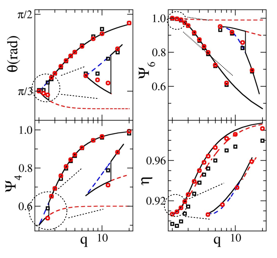
For this reason, in Fig S4 we compare the simulation data for (indicated by black squares) and for (indicated by red circles) with the theoretical values of the perfect rhombatic lattices. Red and blue dashed lines correspond to and structures, respectively. We compare the lattice angle, , the global bond-orientational order parameters, and (defined in the main text), and the packing fraction, . In general, it is observed how the simulation results approach all theoretical quantities and that the agreement improves with increasing pressure. This is particularly true for the packing fraction. Nonetheless, we observe a tendency for the simulation data to depart the theoretical maximal packing fraction as the deformation parameter, , increases, pointing out that an even higher pressure is needed to reach the close-packing limit in case of square-like particles. More importantly, all simulation results are close and below the conjectured maximal packing limit, which supports and as optimal arrangements.
A perfect rhombic lattice has and . These expressions, substituting from Eq.(S10), give the dashed curves of the and panels of Fig. S4. The agreement with the simulations is good. However, in the limiting cases, there appears some discrepancies explained below. For the theoretical curves we have and in the disk limit (, ), and and in the square limit (, ). These limits are not necessarily valid at finite pressure when QLR positional order replaces the long-range order of the perfect lattice. Especially, can be quite different given that the four nearest neighbors of a particle turn ill-defined in the disk limit. Due to the small fluctuations of the particles’ positions and orientations, we get . A similar problem appears with in the square limit.

For the data agree with the curves, whereas they are consistent with the curves for (see the panels corresponding to and ). Similarly, the data obtained for not so high pressure agree with the curves for and with the curves for . Thus, there appears a difference between high and very high pressures for the case (see the inserts in all panels of Fig. S4) that suggests a transition from -like structures to -ones. From the probability density functions, we estimate this transition to be around . This is why we are drawing a tilt dashed line splitting the rhombic solid from the hexagonal solid in the phase diagram (Fig. 3) shown in the manuscript.
VI.5 Results for the case
In this section of the SM, we show the outcomes from REMC simulations for the system with . This case is close to the disk limit and the melting of these particles corresponds to a different scenario, differing from the cases presented in the main text. Namely, there appears a discontinuous two-step melting with a first-order transition between the isotropic and the hexatic phases and a continuous transition between the hexatic and the plastic solid phase. The first-order transition can be clearly read from panel a), which shows how the probability density functions distort from the Gaussian-shape and turn bimodal from to , signaling the coexistence region between the isotropic and the hexatic phases. Note that our low-boundary estimation of this region is smaller than the generally accepted value. This is due to size effects. Furthermore, in this region, we have a plateau in the EOS, a large peak in , and a sudden increase in . We highlight this region with the vertical red dashed lines crossing from panel a) to d). Also, panel e) depicts the change from short-range to QLR behavior of the and panel f) the change from short-range to long-range of , passing through QLR correlations. We estimate the establishment of long-range and QLR for and , respectively, occurring at . We draw a vertical cyan dashed line at this density. All these features are in common with the case, thus we recover the third scenario mentioned in the first paragraph of the main text.
Differences between disks and superdisks with appear above . To begin with, given that particles with break the circular symmetry, the hexagonal solid-phase turns into a plastic phase with hexagonal crystal structure, also called hexagonal solid rotator phase. This phase has QLR positional order, but particle-orientation correlations are short-ranged. The particles orientational degrees of freedom frozen only at very high pressures and high densities to yield an orientationally ordered rhombic solid phase (see the snapshot in Fig. S4). We detect a smooth solid–solid transition, where the Gaussian-shape of all PDFs is preserved, but their height (width) decreases (increases) a little at it. This is accompanied by a small peak of and a sudden increase in . A vertical dashed line is placed across panels a)-d) of Fig. S5 to signal this transition. All these features resemble the behavior of rounded-hard squares Zhao et al. 2012; Avendano and Escobedo 2012, hard ellipses Bautista-Carbajal and Odriozola 2014, and discorectangles Bates and Frenkel 2000 with quasi-circular symmetry.
VI.6 Dimensionless isothermal compressibility and global order parameters
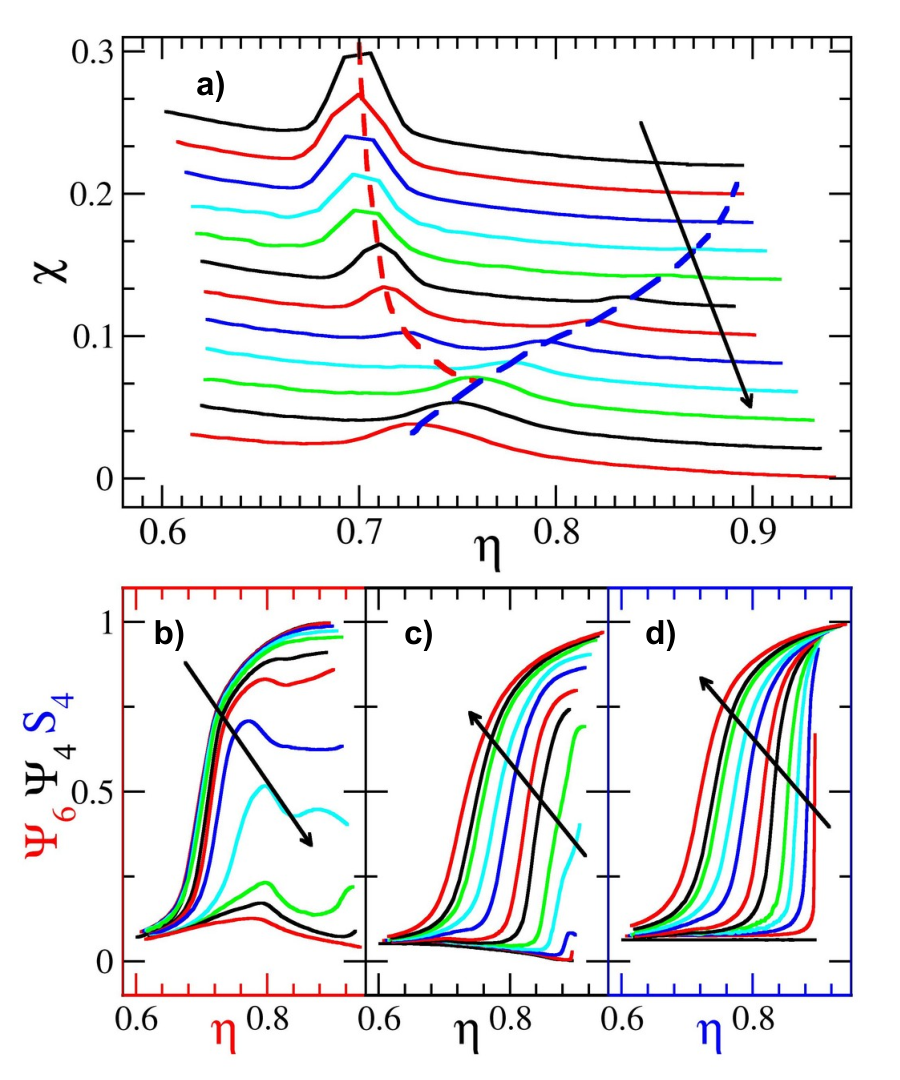
We present here the curves of the dimensionless isothermal compressibility, , and the measured global order parameters as obtained from the REMC as a function of the deformation parameter, . The global order parameters are the six- and four-fold bond-orientational and the tetratic particle orientational ones. The aim of doing this is two-fold. First, we highlight that the REMC technique produces very smooth curves for the isothermal compressibility, which allows for the easy detection of the phase boundaries. This contrasts with the standard point-by-point simulations. Second, we summarize all cases making clear how we build the global phase diagram shown in Fig. 3 of the main text.
The trends of the peaks with increasing are depicted in Fig. S6 a). Note that the peak appearing at low densities shifting to the right correlates with the sudden increase of , whereas the one appearing at high densities correlates with the increase of and . Also, it is observed that the - correlation expands all the interval (see Fig. S6 b) and c)), although the steep increase anticipates that for . We add Y-shaped guides to the eye as red and blue dashed lines in Fig. S6 a), suggesting the vanishing of the isotropic-hexatic transition. The right-hand side branch (blue) of the Y corresponds to the building of orientational order, whereas the left-hand side branch (red) signals the isotropic-hexatic transition.
References
- Murray and Van Winkle (1987) C. A. Murray and D. H. Van Winkle, Phys. Rev. Lett. 58, 1200 (1987).
- Donev et al. (2006) A. Donev, J. Burton, F. H. Stillinger, and S. Torquato, Phys. Rev. B 73, 054109 (2006).
- Han et al. (2008) Y. Han, N. Y. Ha, A. M. Alsayed, and A. G. Yodh, Phys. Rev. E 77, 041406 (2008).
- Halperin and Nelson (1978) B. I. Halperin and D. R. Nelson, Phys. Rev. Lett. 41, 121 (1978).
- Kosterlitz and Thouless (1973) J. M. Kosterlitz and D. J. Thouless, J. Phys. C 6, 1181 (1973).
- Young (1979) A. P. Young, Phys. Rev. B 19, 1855 (1979).
- Anderson et al. (2017) J. Anderson, J. Antonaglia, J. Millan, M. Engel, and S. Glotzer, Phys. Rev. X 7, 021001 (2017).
- Karnchanaphanurach et al. (2000) P. Karnchanaphanurach, B. Lin, and S. A. Rice, Phys. Rev. E 61, 4036 (2000).
- Marcus and Rice (1996) A. H. Marcus and S. A. Rice, Phys. Rev. Lett. 77, 2577 (1996).
- Qi et al. (2014) W. Qi, A. P. Gantapara, and M. Dijkstra, Soft Matter 10, 5449 (2014).
- Thorneywork et al. (2017) A. Thorneywork, J. Abbott, D. Aarts, and R. Dullens, Phys. Rev. Lett. 118, 158001 (2017).
- Wojciechowski and Frenkel (2004) K. W. Wojciechowski and D. Frenkel, Comp. Met. Sci. Technol. 10, 235 (2004).
- Schilling et al. (2005) T. Schilling, S. Pronk, B. Mulder, and D. Frenkel, Phys. Rev. E. 71, 036138 (2005).
- Bernard and Krauth (2011) E. P. Bernard and W. Krauth, Phys. Rev. Lett. 107, 155704 (2011).
- Engel et al. (2013) M. Engel, J. A. Anderson, S. C. Glotzer, M. Isobe, E. P. Bernard, and W. Krauth, Phys. Rev. E 87, 042134 (2013).
- Kapfer and Krauth (2015) S. Kapfer and W. Krauth, Phys. Rev. Lett 114, 035702 (2015).
- Li and Ciamarra (2020) Y.-W. Li and M. P. Ciamarra, Phys. Rev. Lett. 124, 218002 (2020).
- Lyubartsev et al. (1992) A. P. Lyubartsev, A. A. Martinovski, S. V. Shevkunov, and P. N. Vorontsov-Velyaminov, J. Chem. Phys. 96, 1776 (1992).
- Hukushima and Nemoto (1996) K. Hukushima and K. Nemoto, J. Phys. Soc. Jpn. 65, 1604 (1996).
- Okabe et al. (2001) T. Okabe, M. Kawata, Y. Okamoto, and M. Mikami, Chem. Phys. Lett. 335, 435 (2001).
- Basurto et al. (2018) E. Basurto, C. Haro-Pérez, C. A. Vargas, and G. Odriozola, Phys. Chem. Chem. Phys. 20, 27490 (2018).
- Avendano and Escobedo (2012) C. Avendano and F. A. Escobedo, Soft Matter 8, 4675 (2012).
- Zhaglin et al. (2018) H. Zhaglin, Y. Ju, Y.-w. Zong, F.-f. Ye, and K. Zhao, Chinese Physics B 27, 088203 (2018).
- Zhao et al. (2011) K. Zhao, R. Bruinsma, and T. Mason, PNAS 108, 2684 (2011).
- Jiao et al. (2008) Y. Jiao, F. Stillinger, and S. Torquato, Phys. Rev. Lett. 100, 245504 (2008).
- Meijer et al. (2017) J.-M. Meijer, A. Pal, S. Ouhajji, H. N. W. Lekkerkerker, A. P. Philipse, and A. V. Petukhov, Nat. Commun. 8, 14352 (2017).
- Rossi et al. (2015a) L. Rossi, V. Soni, D. J. Ashton, D. J. Pine, A. P. Philipse, P. M. Chaikin, M. Dijkstra, S. Sacanna, and W. T. M. Irvine, Proceedings of the National Academy of Sciences 112, 5286 (2015a).
- Meijer et al. (2019a) J.-M. Meijer, V. Meester, F. Hagemans, H. Lekkerkerker, A. P. Philipse, and A. V. Petukhov, Langmuir 35, 4946 (2019a).
- Mizani et al. (2020) S. Mizani, P. Gurin, R. Aliabadi, H. Salehi, and S. Varga, J. Chem. Phys. 153, 034501 (2020).
- Basurto et al. (2020) E. Basurto, P. Gurin, S. Varga, and G. Odriozola, Phys. Rev. Res. 2, 013356 (2020).
- Rossi et al. (2015b) L. Rossi, V. Soni, D. Ashton, D. Pine, A. Philipse, P. M. Chaikin, M. Dijkstra, S. Sacanna, and W. Irvine, PNAS 112, 5286–5290 (2015b).
- Meijer et al. (2019b) J. Meijer, V. Meester, F. Hagemans, H. Lekkerkerker, A. Philipse, and A. Petukhov, Langmuir 35, 4946 (2019b).
- Zhao et al. (2012) K. Zhao, R. Bruinsma, and T. G. Mason, Nat. Commun. 3, 801 (2012).
- Bautista-Carbajal and Odriozola (2014) G. Bautista-Carbajal and G. Odriozola, J. Chem. Phys. 140, 204502 (2014).
- Bates and Frenkel (2000) M. A. Bates and D. Frenkel, J. Chem. Phys. 112, 10034 (2000).