Reducing the Variance of Variational Estimates of Mutual Information by Limiting the Critic’s Hypothesis Space to RKHS
Abstract
Mutual information (MI) is an information-theoretic measure of dependency between two random variables. Several methods to estimate MI from samples of two random variables with unknown underlying probability distributions have been proposed in the literature. Recent methods realize parametric probability distributions or critic as a neural network to approximate unknown density ratios. These approximated density ratios are used to estimate different variational lower bounds of MI. While, these estimation methods are reliable when the true MI is low, they tend to produce high variance estimates when the true MI is high. We argue that the high variance characteristics is due to the uncontrolled complexity of the critic’s hypothesis space. In support of this argument, we use the data-driven Rademacher complexity of the hypothesis space associated with the critic’s architecture to analyse generalization error bound of variational lower bound estimates of MI. In the proposed work, we show that it is possible to negate the high variance characteristics of these estimators by constraining the critic’s hypothesis space to Reproducing Hilbert Kernel Space (RKHS), which corresponds to a kernel learned using Automated Spectral Kernel Learning (ASKL). By analysing the generalization error bounds, we augment the overall optimisation objective with effective regularisation term. We empirically demonstrate the efficacy of this regularization in enforcing proper bias variance tradeoff on four different variational lower bounds of MI, namely NWJ, MINE, JS and SMILE.
I Introduction
Mutual information is a fundamental information theoretic measure that quantifies the dependency between two random variables (RVs). Given, two RVs, and , mutual information (MI), denoted by is defined as:
Where, is the joint probability distribution and, and are the corresponding marginal distributions. Mutual information, between any two RVs ranges from to . is high when and share considerable information or in other words have a high degree of dependency and vice-versa. It is equal to zero iff and are mutually independent. MI has found wide applications in representation learning [1, 2, 3, 4], generative modeling [5], predictive modeling [6], and information bottleneck [7, 8, 9]. In the learning from data paradigm, data driven applications use sample based estimation of MI, where the key challenge is in estimating MI from the samples of two random variables with unknown joint and marginal distributions.
In the big data regime, with continuous increase in sample size and data dimentionality, reliable estimation of MI using mini-batch stochastic optimisation techniques is an area of active research [10, 11, 12, 13, 14]. Classical non-parametric MI estimators that used methods like binning [15], kernel density estimation [16] and K-Nearest Neighbour based entropy estimation [17] are computationally expensive, produce unreliable estimates, and do not conform to mini-batch based optimisation strategies. To overcome these difficulties, recent estimation methods [11, 12, 13] couple neural networks with variational lower bounds of MI [18, 19] for differential and tractable estimation of MI. In these methods, a critic parameterized as a neural network is trained to approximate unknown density ratios. The approximated density ratios are used to estimate different variational lower bounds of MI. Belghazi et al.[11], Poole et al.[12] and Song et al.[13] consider the universal approximation property of the critic neural network to estimate tighter variational lower bounds of MI. However, universal approximation ability of neural networks comes at the cost of neglecting the effect of critic’s unbounded complexity on variational estimation of mutul information, which leads to unstable and highly fluctuating estimates. Similar observations have been reported in literature by Ghimire et al.in [14].
Nguyen et al.[18] by analysing the bias-variance tradeoff of variational lower bound estimates of MI showed the need to regularise the complexity of the critic’s hypothesis space for stable and low variance estimation of MI. Motivated by their work, we argue that these variational lower bound estimators exhibit high sensitivity to the complexity of critic’s (Neural Network) hypothesis space when optimised using mini-batch stochastic gradient strategy. To support this argument, we use a data-driven measure of hypothesis space complexity called Rademacher complexity to bound the generalization error for variational lower bounds of MI. Using these bounds, it is shown that higher complexity of critic’s hypothesis space leads to higher generalization error and hence high variance estimates. In this proposal, our critic’s hypothesis space is constructed in a smooth family of functions, the Reproducing Kernel Hilbert Space (RKHS). This corresponds to learning a kernel using Automated Spectral Kernel Learning (ASKL) [20]. ASKL parameterized functions in the RKHS as a neural network with cosine activation in the hidden layer. By using the Rademacher complexity of ASKL-RKHS, an effective regularization to control the complexity of the critic’s hypothesis space has also been proposed.
Rest of the paper is organised as follows. Related literature has been reviewed in section II. In section III, we explain some crucial concepts related to our work. The discussion on related work and preliminaries is followed by a detailed explanation of our approach in the section IV where we present a thorough theoretical analysis. Supporting experimental results are demonstrated in section V. For the sake of brevity, all proofs related to our proposal are included in the Appendix.
II Related Work
II-A Mutual Information Estimation
Mutual information can be characterized as the KL divergence between joint distribution and the product of marginal distributions , . This is the central theme in the derivation of lower bounds of MI from variational lower bounds of KL divergence. KL divergence between two multivariate probability distributions, say and belongs to broader class of divergences known as the f-divergences, which are characterized by convex function of likelihood ratio (). Nguyen et al.[18] formulated variational lower bound of f-divergences by using the convex conjugate of and leveraged convex empirical optimization to estimate f-divergences. Belghazi et al.[11] proposed a tighter variational lower bound of KL divergence which is derived from the Donsker-Varadhan [19] dual representation. In their work, two MI estimators are constructed by optimizing neural network critics to maximize (1) convex conjugate lower bound, and (2) Donsker-Varadhan lower bound. In the proposed work, convex conjugate based lower bound estimator is referred to as NWJ and Donsker-Varadhan based estimator as MINE. Poole et al. [12] developed a unified framework for different MI estimates and created an interpolated lower bound for better bias-variance tradeoff. They also proposed a lower bound which is optimized using GAN discriminator objective [21] to estimate density ratios. We refer to the estimator based on this lower bound as JS. Song et al. [13] showed that variance of both MINE and NWJ estimators increase exponentially with increase in the true magnitude of MI. The explained cause of this behaviour is the increase in variance of the partition function estimates [13]. They also proposed a lower bound estimator with improved bias-variance tradeoff by clipping the partition function estimate. In the proposed work, we refer to estimator based on this lower bound as SMILE.
In this approach, instead of designing a better lower bound estimate as proposed in [18, 11, 12, 13], we study the effect of restricting the hypothesis space of critics to RKHS for favourable bias-variance tradeoff. The comparative performance of the proposed work reflects the effectiveness of the proposed approach in learning low variance estimates of MI. Similar to this approach, Ghimire et al.[14] and Ahuja et al.[22] also restricted critic hypothesis space to RKHS. Their methods differ from ours in the choice of kernel functions under consideration. Convex combination of Gaussian kernels were considered in [22]. A stationary Gaussian kernel with inputs transformed by a neural network with randomly sampled output weights has been proposed in [14]. In contrast to the work, we learn a kernel belonging to a much broader class of non-stationary kernels rather than restricting the kernel to Gaussian kernels.
II-B Kernel Learning
Kernel methods play an important role in machine learning [23, 24]. Initial attempts included learning convex [25, 26] or non linear combination [27] of multiple kernels. While the aforementioned kernel learning methods are an improvement over the isotropic kernels, they cannot be used to adapt any arbitrary stationary kernel. To alleviate this problem [28, 29] proposed approximating kernels by learning a spectral distribution. At the core of these methods is Bochner’s theorem [30], which states that there exists a duality between stationary kernels and distributions in spectral domain (Fourier domain). Similarly, Yaglom’s theorem [31] states that there is a duality between the class of kernels and positive semi-definite functions with finite variations in spectral domain. Kom Samo et al.[32] showed that kernels constructed using Yaglom’s theorem are dense in the space of kernels. Ton et al. [33] used Monte- Carlo integration and Yaglom’s theorem to construct non-stationary kernels for Gaussian Processes. Recent methods combine deep learning with kernel learning methods. Deep Kernel Learning [34] placed a plain deep neural network as the front-end of a spectral mixture kernel to extract features, which is further extended to a kernel interpolation framework [35] and stochastic variational inference [36]. Chun-Liang Li et al. [37] modeled the spectral distribution as an implicit generative model parameterized by a neural network and approximated a stationary kernel by performing Monte-Carlo integration using samples from the implicit model. Hui Xue et al.[38] and Jian Li et al.[20] (ASKL) represented a non-stationary kernel as Monte-Carlo integration of fixed samples which are optimized using gradient descent methods. In this work, ASKL is used to learn the kernel corresponding to the critic’s hypothesis space in Reproducing Kernel Hilbert Space.
III Preliminary
III-A Variation Lower Bounds of Mutual Information
In this subsection, four different variational lower bounds namely , , and based estimators of MI have been discussed. These estimators are used in throughout this work. In estimating variational lower bounds of MI, a parametric probability distribution or critic with trainable parameters is optimised to approximate the likelihood density ratio between the joint and product of marginal distributions (). The approximated density ratio is used for sample based estimation of MI. The optimisation objective is to maximize the different variational lower bounds of MI with respect to the critic parameters to estimate MI.
Donsker-Varadhan dual representation [19] based variational lower bound of MI, denoted as is given by:
| (1) |
The optimal critic for which the equality holds in (1) is given by . and lower bounds can be derived from Tractable Unnormalized Barber and Argakov (TUBA) lower bound, , considering only constant positive baseline in [12], that is in the formulation defined as:
| (2) |
Optimal critic satisfying the equality in equation 2 is given by, . In this work, is formulated from by fixing the parameter in (2) as exponential moving average of across mini-batches. Similarly, is formulated from by substituting the parameter .
Unlike the methods described above that maximize the variational lower bounds to learn likelihood density ratio, other methods [12, 13, 2] approximate the density ratio for sample based estimation of MI by optimizing GAN discriminator objective defined as:
| (3) |
Where, is the sigmoid function. The optimal critic maximizing the GAN discriminator objective is given by, . Poole et al.[12] observed that , where is the optimal critic for and constructed another variational lower bound by substituting as the critic function into (2). The is optimized using the GAN discriminator objective. Similarly, Song et al.[13] constructed another lower bound of MI, denoted as by substituting as critic in expressed in (1). In [13], the bias-variance tradeoff is controlled by clipping the critic output. It is essential to note that we do not clip the output of the ASKL critic to analyse the effectiveness of restricting the critic function hypothesis space to Reproducing Kernel Hilbert Space in controlling bias-variance tradeoff.
III-B Automated Spectral Kernel Learning
.
In this subsection we discuss Reproducing Hilbert Kernel Spaces (RKHS) and Automated Spectral Kernel Learning (ASKL). Hilbert space , is an vector space of real valued functions with defined inner product between two functions and . Function norm in the hilbert space is defined as . Reproducing kernel of a hilbert space is a positive semi-definite function, which satisfies the conditions: (1) , and (2) . The latter of the two condition is known as the reproducing property of the kernel [39]. A Hilbert space which posses a reproducing kernel is called a Reproducing Kernel Hilbert Space.
There exist many feature mappings, , where is a Hilbert space, such that and , , and . A special case of such feature mappings known as implicit feature mapping is and .
Yaglom’s theorem [31] as stated below shows that there exists a duality between a positive semidefinite kernel function and a non-negative Lebesgue-Stieltjes measure in spectral domain.
Theorem 1
(Yaglom’s theorem) A kernel is positive semi-definite iff it can be expressed as
where, is Lebesgue-Stieltjes measure associated to some positive semi-definite function with bounded variations.
With appropriate scaling the Lebesgue-Stieltjes measure can be treated as a probability distribution in spectral domain where and are spectral variables. From here on, this probability distributions is referred to as spectral distribution. An implication of theorem 1 is that it is possible to learn an RKHS associated with a kernel by learning a spectral distribution.
Automated Spectral Kernel Learning (ASKL) [20] is a kernel learning method that used samples from the spectral distribution to construct a feature mapping defined as,
| (4) |
Where, and are matrices of frequency samples and and are vectors of uniform samples . The kernel associated with the spectral distribution can be approximated using the feature mapping defined above as . This feature mapping produces a -dimensional embedding in an RKHS for any input . Any function in this RKHS is represented by a -dimensional vector , such that .
ASKL represented the RKHS generated by the above feature mapping as a two layer neural network with cosine activations shown in Fig. 1. The hidden layer of this neural network represents the feature mapping , its trainable parameters are the frequency samples from spectral distribution . The parameters of the final output layer represent functions in the RKHS. The output of the final layer is the inner product . A RKHS can be learned by optimizing this neural network using a stochastic gradient descent method. During the optimization, a spectral distributions is learned implicitly through learning the parameters of the hidden layer . In this work, the critic’s hypothesis space is restricted to an RKHS using the neural network architecture Fig. 1 and ASKL. For more information on ASKL refer to [20]. Any further reference to ASKL critic refers to the neural network architecture shown in Fig. 1.
IV Theory & Our Approach
Our goal is to estimate the mutual information, , between two RVs and , from i.i.d samples, from joint distribution and i.i.d samples, from the product of marginal distributions . As, the true underlying probability distributions are unknown, we use empirical approximations of the variational lower bounds of MI defined as:
| (5) | ||||
| (6) |
Where, is the set of n,m i.i.d samples. , and are empirical distributions corresponding to samples and , respectively, and .
IV-A Theoretical Guarantees
In this subsection the generalization behaviour of the empirical estimates, and are discussed. We derive generalization error bound for the empirical estimates using data-driven Rademacher complexity of general critic’s hypothesis space. We also bound the empirical Rademacher complexity of the ASKL critic’s hypothesis space.
Generalization error quantifies the out of sample behaviour of an estimator. Formally, generalization error is defined as the maximum possible deviation of the empirical estimates from true values. If empirical estimate is an unbiased estimate, then variance of this empirical estimate is upper bounded by the expectation of squared generalization error. Hence, generalization error is an indicator of the variance of the estimate. The following theorem bounds the generalization error of and .
Theorem 2 (Generalization Error Bounds)
Assume, that the hypothesis space of the critic is uniformly bounded by , that is , . For a fixed generalization errors of and can be bounded with probability of at least , given by
| (7) |
| (8) |
Where, sample set for and is assumed to be known, and and are empirical Rademacher averages of the hypothesis space for different sample sizes.
To formulate the generalization error bounds given in the above theorem, we used McDairmid’s inequality to bound generalization error by expected generalization error over sample set . Then we use lemma A5 given in [40] to bound the expected error by Rademacher complexity. Further, Rademecher concentration inequality, lemma A4 also given in [40] is used to arrive at the final theoretical guarantees. Refer to Appendix B for detailed proof. Error bounds for and are derived by substituting the parameter in bound 7 with , and with exponential moving average of across mini-batches, respectively. uses lower bound to estimate MI, hence generalization error of is bounded by generalization error bound of . Similarly, uses lower bound to estimate MI and its generalization error is bounded by error bound of
The generalization error bounds depend on the empirical Rademacher complexities and . Our finding on the dependence of the generalization error on is confirmed by similar observation made in [41] on the sample complexity of MINE estimator. From the error bounds, it can be inferred that high empirical Rademacher complexity of the critic’s hypothesis space leads to high generalization error, hence high variance estimates. Therefore, variance of these estimates can be effectively reduced by choosing a hypothesis space for critic with low Rademacher complexity. However, it is also necessary to keep the hypothesis space rich enough to induce low bias. Though these bounds apply to all hypothesis spaces including the space of functions that are learned by a fully connected neural network, emperical estimation of Rademacher complexity for a fully connected neural network is an open area of research. We restrict the critic neural networks hypothesis space to RKHS by using ASKL to gain insights into variational lower bound estimates of MI. The empirical Rademacher complexity of the ASKL critic’s hypothesis space can be upper bounded as shown by the following theorem,


Theorem 3
The empirical Rademacher average of the RKHS to which ASKL critic belongs can be bounded as following
Where .
We used the Cauchy-Schwarz inequality to bound the complexity of the ASKL critic, for detailed proof refer to Appendix A. Note that, the second inequality in the above theorem is true only in the case of ASKL critic. Using the above theorem we can decrease the complexity by decreasing the largest possible norm of RKHS representation of functions or decreasing the frobenius norm of the feature mapping matrix. In the next subsection, we present an optimization procedure to decrease the empirical Rademacher complexity by penalizing and to control the bias-variance tradeoff. Using second inequality, and penalizing it is possible to carve out the regularisation used by Nguyen et al.[18] to control hypothesis space complexity.
IV-B Training Methodology
We train an ASKL critic neural network shown in Fig. 1 to simultaneously maximize empirical estimate of MI and minimize regularization terms defined below. The overall training objective is:
| (9) |
Where, can be an empirical estimate of any variational lower bound of MI, , , or . And is the set of trainable parameters , , and . GAN discriminator objective is maximized in cases where is or . In this work, regularization terms and appear in upper bound of empirical Rademacher complexity of ASKL critic’s hypothesis space. Bias-variance tradeoff is controlled by tuning hyperparameters, and . We use mini-batch stochastic gradient decent to train the estimator.
V Experiments
| Lower Bound | ||
|---|---|---|
| NWJ[42] | 0.001 | 0.001 |
| MINE[11] | 0.001 | 0.001 |
| JS[12] | 1e-5 | 1e-5 |
| SMILE[13] | 1e-4 | 0.001 |
We empirically validate our claims on two different toy datasets which have been widely used by other MI estimation methods [11, 12, 13], (1) correlated Gaussian dataset, where samples of two RVs are drawn from a 20 dimensional Gaussian distribution with correlation between each dimension of and . The correlation is increased such that increases in steps of 2 every 4000 training steps, and (2) cubed Gaussian dataset, same as in (1) but we apply a cubic non-linearity to to get samples (, ). As, mutual information remains unchanged by application of deterministic functions on random variables, . Further, is it important to note that previous methods increased the correlation till the true MI is increased to 10. In our experimental analysis, we increased the correlation till the true MI is 20 to demonstrate that ASKL critic produces low variance estimates even at high values of MI.
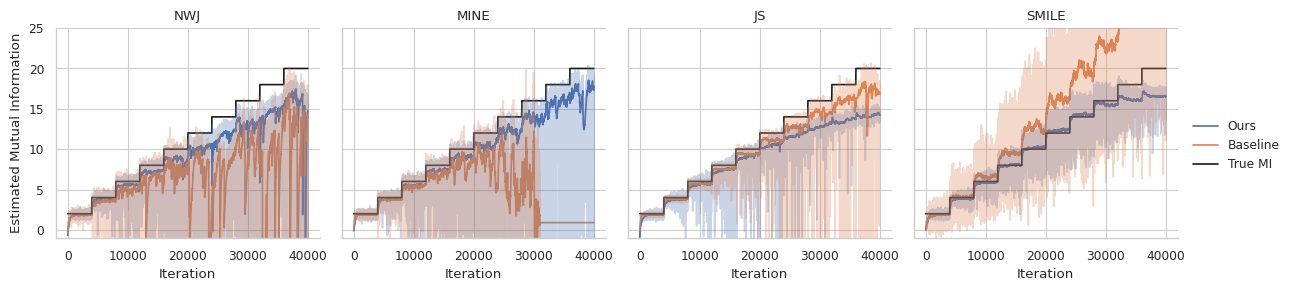
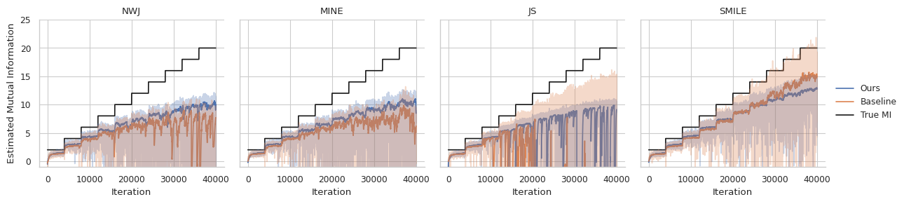
For comparative analysis we train ASKL critic and a baseline critic on four different lower bounds, namely , , , and . The baseline critic is a fully connected neural network with ReLU activations. This baseline has been used by previous estimation methods that consider the universal approximation property of neural networks [11, 12, 13]. ASKL critic with regularised space complexity computes low variance stable variational lower bound estimates of MI in comparison to baseline critic.
Code for this paper are available at https://cvit.iiit.ac.in/projects/mutualInfo/.


V-A Training Details
For ASKL critic, is set to 512, that is 512 spectral samples are used for estimation. The multiplicity factors for each of the regularization terms used for different estimators are given in Table I. For our baseline critic, we used a 3 layer neural network with 256 units in each hidden layer. Unless mentioned otherwise, batch size is set to 64. We use Adam optimizer [43] with and . Learning rates are set to and for ASKL and baseline critics, respectively.
We test the validity of our claim that constraining the critic to RKHS should lead to better bias-variance tradeoff in three different experimental setups, (1) qualitatively compare the variance of MI estimates between ASKL critic and baseline critic on four different variational lower bounds of MI. These experiments are performed on both toy datasets described above, batch size is fixed at 64 sample, (2) quantitatively compare the average bias, variance, and the root mean square error (RMSE) between the true and empirical estimates of MI over 50 experimental trials. These quantitative comparisons are made over a range of batch sizes to depict the robustness of our estimates with varying batch sizes, (3) quantitatively demonstrate the efficacy of the proposed regularisation terms in controlling bias-variance tradeoff of ASKL critic’s space complexity by varying the regularisation hyperparameters and for and , respectively. In experiment (3), bias-variance values are estimated over 50 experiments. Both experients (1) and (2) are run on correlated Gaussian dataset. We further elaborate on each of these experimental results in the next subsection.
V-B Results
Qualitative comparison between ASKL critic and baseline critic on four different variational lower bounds of MI has been shown in Fig. 2. Fig. 2(a) and Fig. 2(b) demonstrate the comparative results on the 20 dimensional correlated Gaussian dataset and the cubed correlated Gaussian dataset, respectively. In can be seen that maximisation using ASKL critic tends to produce stable estimates in comparison to their baseline counterpart. A particular instance of numerical instability in baseline critic estimates can be observed in the plot corresponding to when the true MI is higher than 16. Estimates by ASKL critic does not suffer from such instability and it is to be noted that the ASKL critic also produces comparatively low variance MI.
We compute bias, variance, and root mean square error of the estimated MI values to quantitatively evaluate the proposed ASKL critic’s performance against the baseline. The bias, variance, and RMSE values have been averaged over 50 experimental trials. Fig. 3(a) and Fig. 3(b) show the computed values for the ASKL critic and the baseline, respectively. These plots conclusively demonstrate that the ASKL critic estimates have lower bias and variance characteristics in comparison to the baseline critic. Lower variance characteristics of the ASKL critic can be explained by observing that the empirical Rademacher complexity of ASKL critic’s hypothesis space is bounded, theorem 3. Hence, generalization error is guaranteed to be upper bounded. Lower bias in estimates can be attributed to better control over bias-variance tradeoff.
Experimental results shown in Fig. 3, demonstrates the effect of change in batch size on the variance of ASKL and baseline critic estimates. It can be observed that with an increase in batch size the variance of both ASKL and baseline estimates decreases. This is due to the fact that the empirical Rademacher complexity is inversely proportional to the sample size (refer Appendix A for definition). Hence, an increase in batch size leads to a decrease in empirical Rademacher complexity and, corresponding decrease in variance of the MI estimates. Another key observation on the variance of MI estimates which holds for both critics is that with an increase in true MI the variance of the empirical estimates increases. This observations can be explained by noticing the effect of increase in the value of true MI on the log likelihood density ratio between the joint and product of marginal distributions, . The absolute value of the log density ratio evaluated at any given sample increases with increase in MI. The optimal critics for variational lower bound estimates of MI depend on the log density ratio. Hence, to match the increase in log density ratio the constant which uniformly bounds the critic’s hypothesis space also increases. As described in theorem 2, the generalization error bounds depend on both empirical Rademacher complexity and , hence, an increase in leads to an increase in variance of MI estimates.
Bias-variance tradeoff for different values of and in ASKL critic, figure 4. Figures 4(a) and 4(b) are the bias and variance plots, respectively. The left top most plots in both figures, 4(a) and 4(b) correspond to and set to 0, respectively. It can be seen in these plots that even without any explicit regularisation estimates using ASKL critic have lower bias and lower variance in comparison to the baseline critic. This verifies our claim that constraining the complexity of the hypothesis space leads to significant improvement in reliability of these estimates. It is evident from these plots that regularization weights are also effective in controlling the bias, as and increase the estimates get biased in negative direction. This demonstrates the efficacy of the proposed regularization terms in inducing effective bias-variance tradeoff.
VI Conclusion
In the proposed work, we successfully demonstrate the effect of controlling the complexity of critic’s hypothesis space on the variance of sample based empirical estimates of mutual information. We negate the high variance characteristics of variational lower bound based estimates of MI by constructing the critic’s hypothesis space in a Reproducing Kernel Hilbert Space, which corresponds to a critic learned using Automated Spectral Kernel Learning architecture. By analysing the generalisation bounds using Radmacher complexity of the constrained critic space, we demonstrate effective regularisation of bias-variance tradeoff on four different variational lower bounds of Mutual information. In larger scheme of Explainable-AI, this work theoretically motivates the implications of understanding the effect of regulating the complexity of deep neural network based critic hypothesis spaces on the bias-variance tradeoff of variational lower bound estimators of mutual information.
References
- [1] T. Q. Chen, X. Li, R. B. Grosse, and D. K. Duvenaud, “Isolating sources of disentanglement in variational autoencoders,” in Advances in Neural Information Processing Systems, 2018, pp. 2610–2620.
- [2] H. Kim and A. Mnih, “Disentangling by factorising,” arXiv preprint arXiv:1802.05983, 2018.
- [3] A. A. Alemi, B. Poole, I. Fischer, J. V. Dillon, R. A. Saurous, and K. Murphy, “Fixing a broken elbo,” arXiv preprint arXiv:1711.00464, 2017.
- [4] R. D. Hjelm, A. Fedorov, S. Lavoie-Marchildon, K. Grewal, P. Bachman, A. Trischler, and Y. Bengio, “Learning deep representations by mutual information estimation and maximization,” arXiv preprint arXiv:1808.06670, 2018.
- [5] X. Chen, Y. Duan, R. Houthooft, J. Schulman, I. Sutskever, and P. Abbeel, “Infogan: Interpretable representation learning by information maximizing generative adversarial nets,” in Advances in neural information processing systems, 2016, pp. 2172–2180.
- [6] Y. Li, “Which way are you going? imitative decision learning for path forecasting in dynamic scenes,” in The IEEE Conference on Computer Vision and Pattern Recognition (CVPR), June 2019.
- [7] N. Tishby, F. C. Pereira, and W. Bialek, “The information bottleneck method,” arXiv preprint physics/0004057, 2000.
- [8] N. Tishby and N. Zaslavsky, “Deep learning and the information bottleneck principle,” in 2015 IEEE Information Theory Workshop (ITW). IEEE, 2015, pp. 1–5.
- [9] A. A. Alemi, I. Fischer, J. V. Dillon, and K. Murphy, “Deep variational information bottleneck,” arXiv preprint arXiv:1612.00410, 2016.
- [10] A. v. d. Oord, Y. Li, and O. Vinyals, “Representation learning with contrastive predictive coding,” arXiv preprint arXiv:1807.03748, 2018.
- [11] M. I. Belghazi, A. Baratin, S. Rajeshwar, S. Ozair, Y. Bengio, A. Courville, and D. Hjelm, “Mutual information neural estimation,” in International Conference on Machine Learning, 2018, pp. 531–540.
- [12] B. Poole, S. Ozair, A. van den Oord, A. A. Alemi, and G. Tucker, “On variational lower bounds of mutual information,” in NeurIPS Workshop on Bayesian Deep Learning, 2018.
- [13] J. Song and S. Ermon, “Understanding the limitations of variational mutual information estimators,” arXiv preprint arXiv:1910.06222, 2019.
- [14] S. Ghimire, P. K. Gyawali, and L. Wang, “Reliable estimation of kullback-leibler divergence by controlling discriminator complexity in the reproducing kernel hilbert space,” arXiv preprint arXiv:2002.11187, 2020.
- [15] A. M. Fraser and H. L. Swinney, “Independent coordinates for strange attractors from mutual information,” Physical review A, vol. 33, no. 2, p. 1134, 1986.
- [16] Y.-I. Moon, B. Rajagopalan, and U. Lall, “Estimation of mutual information using kernel density estimators,” Physical Review E, vol. 52, no. 3, p. 2318, 1995.
- [17] A. Kraskov, H. Stögbauer, and P. Grassberger, “Estimating mutual information,” Physical review E, vol. 69, no. 6, p. 066138, 2004.
- [18] X. Nguyen, M. J. Wainwright, and M. I. Jordan, “Estimating divergence functionals and the likelihood ratio by convex risk minimization,” IEEE Transactions on Information Theory, vol. 56, no. 11, pp. 5847–5861, 2010.
- [19] M. D. Donsker and S. S. Varadhan, “Asymptotic evaluation of certain markov process expectations for large time. iv,” Communications on Pure and Applied Mathematics, vol. 36, no. 2, pp. 183–212, 1983.
- [20] J. Li, Y. Liu, and W. Wang, “Automated spectral kernel learning,” arXiv preprint arXiv:1909.04894, 2019.
- [21] I. Goodfellow, J. Pouget-Abadie, M. Mirza, B. Xu, D. Warde-Farley, S. Ozair, A. Courville, and Y. Bengio, “Generative adversarial nets,” in Advances in neural information processing systems, 2014, pp. 2672–2680.
- [22] K. Ahuja, “Estimating kullback-leibler divergence using kernel machines,” arXiv preprint arXiv:1905.00586, 2019.
- [23] J. Shawe-Taylor, N. Cristianini et al., Kernel methods for pattern analysis. Cambridge university press, 2004.
- [24] B. Scholkopf and A. J. Smola, Learning with kernels: support vector machines, regularization, optimization, and beyond. MIT press, 2001.
- [25] G. R. Lanckriet, N. Cristianini, P. Bartlett, L. E. Ghaoui, and M. I. Jordan, “Learning the kernel matrix with semidefinite programming,” Journal of Machine learning research, vol. 5, no. Jan, pp. 27–72, 2004.
- [26] C. Cortes, M. Mohri, and A. Rostamizadeh, “L2 regularization for learning kernels,” arXiv preprint arXiv:1205.2653, 2012.
- [27] ——, “Learning non-linear combinations of kernels,” in Advances in neural information processing systems, 2009, pp. 396–404.
- [28] A. Wilson and R. Adams, “Gaussian process kernels for pattern discovery and extrapolation,” in International conference on machine learning, 2013, pp. 1067–1075.
- [29] M. Lázaro-Gredilla, J. Quiñonero-Candela, C. E. Rasmussen, and A. R. Figueiras-Vidal, “Sparse spectrum gaussian process regression,” The Journal of Machine Learning Research, vol. 11, pp. 1865–1881, 2010.
- [30] W. Rudin, Fourier analysis on groups. Wiley Online Library, 1962, vol. 121967.
- [31] A. M. Yaglom, “Correlation theory of stationary and related random functions.” Volume I: Basic Results., vol. 526, 1987.
- [32] Y.-L. K. Samo and S. Roberts, “Generalized spectral kernels,” arXiv preprint arXiv:1506.02236, 2015.
- [33] J.-F. Ton, S. Flaxman, D. Sejdinovic, and S. Bhatt, “Spatial mapping with gaussian processes and nonstationary fourier features,” Spatial statistics, vol. 28, pp. 59–78, 2018.
- [34] A. G. Wilson, Z. Hu, R. Salakhutdinov, and E. P. Xing, “Deep kernel learning,” in Artificial Intelligence and Statistics, 2016, pp. 370–378.
- [35] A. Wilson and H. Nickisch, “Kernel interpolation for scalable structured gaussian processes (kiss-gp),” in International Conference on Machine Learning, 2015, pp. 1775–1784.
- [36] A. G. Wilson, Z. Hu, R. R. Salakhutdinov, and E. P. Xing, “Stochastic variational deep kernel learning,” in Advances in Neural Information Processing Systems, 2016, pp. 2586–2594.
- [37] C.-L. Li, W.-C. Chang, Y. Mroueh, Y. Yang, and B. Póczos, “Implicit kernel learning,” arXiv preprint arXiv:1902.10214, 2019.
- [38] H. Xue, Z.-F. Wu, and W.-X. Sun, “Deep spectral kernel learning,” in Proceedings of the 28th International Joint Conference on Artificial Intelligence. AAAI Press, 2019, pp. 4019–4025.
- [39] A. Berlinet and C. Thomas-Agnan, Reproducing kernel Hilbert spaces in probability and statistics. Springer Science & Business Media, 2011.
- [40] P. L. Bartlett, O. Bousquet, S. Mendelson et al., “Local rademacher complexities,” The Annals of Statistics, vol. 33, no. 4, pp. 1497–1537, 2005.
- [41] D. McAllester and K. Stratos, “Formal limitations on the measurement of mutual information,” arXiv preprint arXiv:1811.04251, 2018.
- [42] S. Nowozin, B. Cseke, and R. Tomioka, “f-gan: Training generative neural samplers using variational divergence minimization,” in Advances in neural information processing systems, 2016, pp. 271–279.
- [43] D. P. Kingma and J. Ba, “Adam: A method for stochastic optimization,” arXiv preprint arXiv:1412.6980, 2014.