Relativistic EOM-CCSD for core-excited and core-ionized state energies based on the 4-component Dirac-Coulomb(-Gaunt) Hamiltonian
Abstract
We report an implementation of the core-valence separation approach to the 4-component relativistic Hamiltonian based equation-of-motion coupled-cluster with singles and doubles theory (CVS-EOM-CCSD), for the calculation of relativistic core-ionization potentials and core-excitation energies. With this implementation, which is capable of exploiting double group symmetry, we investigate the effects of the different CVS-EOM-CCSD variants, and the use of different Hamiltonians based on the exact 2-component (X2C) framework, on the energies of different core ionized and excited states in halogen (CH3I, HX and X-, X = Cl-At) and xenon containing (Xe, XeF2) species. Our results show that the X2C molecular mean-field approach [Sikkema et al. J. Chem. Phys. 2009, 131, 124116], based on 4-component Dirac-Coulomb mean-field calculations (2DCM) is capable of providing core excitations and ionization energies that are nearly indistinguishable from the reference 4-component energies for up to and including fifth-row elements. We observe that two-electron integrals over the small-component basis sets yield non-negligible contributions to core binding energies for the K and L edges for atoms such as iodine or astatine, and that the approach based on Dirac-Coulomb-Gaunt mean-field calculations (2DCGM) are significantly more accurate than X2C calculations for which screened two-electron spin-orbit interactions are included via atomic mean-field integrals.
I Introduction
X-ray spectroscopies, which typically probe core electrons through electronic excitation or ionization, are particularly suitable techniques to study the local environment of atoms, molecules and materials, as the localized nature of the core orbitals makes them very selective and sensitive. Stöhr 1992; Norman and Dreuw 2018
Over the last few years, new X-ray free electron lasers (XFEL) and last generation synchrotrons have started operating. These advanced light sources have opened the door to a variety of new X-ray-based spectroscopies, van Bokhoven and Lamberti 2016; Mobilio, Boscherini, and Meneghini 2014; Bergmann, Yachandra, and Yano 2017 including those operating in time-resolved and non-linear regimes.van Bokhoven and Lamberti 2016; Mobilio, Boscherini, and Meneghini 2014; Bergmann, Yachandra, and Yano 2017; Nisoli et al. 2017; Norman and Dreuw 2018 As stated for instance by Milne, Penfold and Chergui in their review: Milne, Penfold, and Chergui 2014 “[…] The progress of experimental techniques for core level spectroscopies is unraveling subtle spectral features implying that high level theoretical approaches are required to interpret them […]”. The experimental X-ray spectra need to be compared to highly accurate theoretical calculations to assign spectral features and to relate experimental measurements to the structure and dynamic properties of the probed molecular system.
Among the methods one can use to calculate core binding energies SCF Bagus 1965; Bagus and Schaefer 1971 stands out due to the combination of low computational cost and good results. By performing separate SCF calculations on the original (generally neutral, and closed-shell) and ionized (generally open-shell) species, it introduces the important orbital relaxation that accompanies the creation of the core hole, though at the expense of requiring several calculations for the edges of interest, and with the potential complication that the required open-shell calculations may be difficult to converge. The same approach can be applied in a straightforward manner to DFT, Besley 2021 with the additional complication that it will show a certain dependence on the chosen density functional. The same idea of performing separate calculations for the initial and the target states can be used to devise approaches based on correlated wavefunctions such as MP2 South et al. 2016 or coupled-cluster (CC). Zheng and Cheng 2019; Lee, Small, and Head-Gordon 2019 Analogous methods for core excitations have also been formulated,Besley, Gilbert, and Gill 2009; Liang et al. 2017; Hait and Head-Gordon 2020; Ehlert and Klamroth 2020; Derricotte and Evangelista 2015; Verma, Derricotte, and Evangelista 2016; Hunt and Goddard 1969; Ågren et al. 1994; Ferré and Assfeld 2002 though this has proven somewhat more cumbersome than for ionizations, since one has to select orbital pairs that should represent the transitions, and converge such excited configurations. In a number of these approaches the orbitals for the ground and excited/ionized states are not orthogonal, making for instance the calculation of transition moments more involved.
The difficulties above are circumvented with approaches that diagonalize the same Hamiltonian for both the original and the ionized or excited states. As such, excited state approaches based on wavefunction theory, like, for instance, (multireference) configuration interaction (MRCI), Lundberg and Delcey 2019; Bokarev and Kühn 2020; Klooster, Broer, and Filatov 2012; Maganas et al. 2019 equation of motion CC (EOM-CC)Coriani et al. 2012; Coriani and Koch 2015; Coriani and Koch 2016; Sadybekov and Krylov 2017; Vidal et al. 2019; Peng et al. 2015; Paul, Myhre, and Koch 2021; Park, Perera, and Bartlett 2019; Matthews 2020 and multireference (EOM)CC,Brabec et al. 2012; Maganas et al. 2019 and linear response complete active space SCF (LR-CASSCF), Helmich-Paris 2021 on Green’s functions such as the algebraic diagrammatic construction (ADC), Schirmer and Thiel 2001; Wenzel, Wormit, and Dreuw 2014; Dreuw and Wormit 2015; Neville et al. 2016 or on time-dependent density functional theory (TDDFT), Besley 2021; Ekström et al. 2006; Besley 2020 can all be used to target core excited or ionized states. One downside is, however, that now relaxation has to be accounted for by the correlated electronic structure approach. Among these, single-reference CC methods, and in particular those based on EOM and the closely related linear response (LRCC) formalisms, Stanton and Bartlett 1993; Sneskov and Christiansen 2012; Bartlett 2012; Krylov 2008; Christiansen, Jørgensen, and Hättig 1998; Koch and Jørgensen 1990; Coriani et al. 2016 are capable of treating electron correlation accurately and in a balanced way between ground and excited states, including a good deal of relaxation effects, and have an appealing “black box” nature (though they are less adept than MRCI/MRCC at treating cases for which the ground state shows a strong multireference nature).
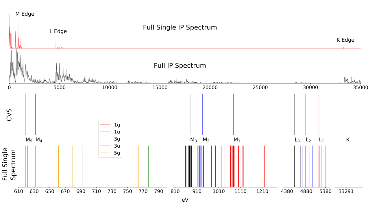
Irrespective of the correlated method, a particular difficulty for determining core states by diagonalizing a many-body Hamiltonian is that such states appear at high energies, where spectra are potentially very dense (see for example figure 2). Thus, a naive application of procedures which target exterior roots (such as the Davidson algorithm), would require solving for a very large number of roots. One way to overcome this issue is through the use of methods capable of solving for interior roots without requiring that all of them are targeted, as those recently devised and applied to multiconfigurational, Helmich-Paris 2021 EOMCC Zuev et al. 2015; Peng et al. 2015 and mean-field Huang et al. 2017; Huang and Liu 2019 wavefunctions.
A more widespread strategy, Stener, Fronzoni, and de Simone 2003; Schirmer and Thiel 2001; Wenzel, Wormit, and Dreuw 2014; Dreuw and Wormit 2015; Coriani and Koch 2015; Coriani and Koch 2016; Vidal et al. 2019; Tenorio et al. 2019; Seidu et al. 2019; Lundberg and Delcey 2019; Helmich-Paris 2021; Delcey et al. 2019; Matthews 2020; Park, Perera, and Bartlett 2019 which we follow in this paper, is to employ physically motivated approximations to the original Hamiltonian, in particular within the core valence separation (CVS) approximation.Cederbaum, Domcke, and Schirmer 1980 The core-valence separation is justified by the large spatial and energetic separation between valence and core orbitals/electrons. On the one side, CVS allows to straightforwardly address the highly-energetic core states with minor modifications to preexisting eigenvalue solvers. On the other side, the CVS helps alleviating convergence issues due to the large number of valence ionized states in the frequency region of the core excitations, which is particularly afflicting methods that explicitly include double excitations in their parametrization. Faber and Coriani 2020; Nanda et al. 2020 One can also regard the core states as metastable Feshbach resonances embedded in the (valence) ionization continuum, and application of CVS helps stabilizing them. Further details on the CVS approach will be given in section II.3.
A second issue to be addressed for core states is the importance of relativistic effects, Dyall and Faegri Jr 2007; Saue 2011; Liu 2020 which significantly alter the energies of inner electrons, and consequently the core spectra of atoms and molecules: due to the high velocities of their electrons (a significant fraction of the speed of light), core and orbitals contract (with an associated lowering of their orbital energies) while, due to increased screening, and orbitals expand (with an associated increase in their orbital energies). At the same time, orbitals which are degenerate in a non-relativistic framework (, , ) are (strongly) split due to spin-orbit coupling, and particularly so for the innermost orbitals.
Relativistic effects are so pronounced in the core region that, even for molecules containing only elements of the first and second rows, they are very important for the accurate determination of K and L edge spectra. While rather approximate treatments of relativistic effect can yield accurate results for light elements, Zheng and Cheng 2019; Carbone et al. 2019; Liu et al. 2019; Vidal et al. 2020; Keller et al. 2020 a more consistent way of treating these effects is through an electronic Hamiltonian based on the 4-component Dirac operator, as it is accurate all the way down to the heaviest elements (5d and 6d transition metals, lanthanides and actinides). As such, 4-component based methods are ideally suited to treat the core spectra across the periodic table, and to probe K, L and M edges of heavy elements, Fillaux et al. 2007; Bagus, Ilton, and Nelin 2013; South et al. 2016 which are much more complex to interpret than those of lighter elements. Though the availability of efficient implementations Repisky et al. 2020; Belpassi et al. 2020; Zhang et al. 2020 has in recent years enabled mean-field 4-component calculation for large-scale applications, the additional basis sets required to represent the small component part of the molecular spinors still places a considerable burden on such calculations compared to the non-relativistic case.
An important development to overcome such issues has been the introduction of the so-called eXact 2-Component (X2C) methods Kutzelnigg and Liu 2005; Jensen 2005; Liu and Peng 2006; Iliaš and Saue 2007; Peng et al. 2007; Liu and Peng 2009; Sikkema et al. 2009, in which a transformation to decouple the positive and negative energy states of the Dirac Hamiltonian is available in matrix form and, unlike its more approximate counterparts, yields exactly the same positive energy spectrum as the original 4-component Hamiltonian. We refer the reader to a recent, comprehensive review on relativistic electronic structure for more details Liu 2020.
We note that among the different X2C variants, those that construct the transformation matrix on the basis of converged 4-component atomic or molecular mean-field calculations Liu and Peng 2006; Peng et al. 2007; Sikkema et al. 2009 are particularly interesting to correlated calculations Sikkema et al. 2009; Liu et al. 2018; Liu and Cheng 2018; Cheng 2019; Asthana, Liu, and Cheng 2019, since they avoid the handling of two-electron integrals over small component basis functions in the transformation to molecular spinors, while largely avoiding errors with respect to the original 4-component Hamiltonian on the description of two-electron spin-orbit coupling contributions, compared to approaches in which the decoupling is performed based on the one-electron Dirac Hamiltonian prior to the mean-field step Iliaš and Saue 2007.
In this study, we present an approach to study core ionization (and excitation) through the use of projectors, inspired by the work of Coriani and Koch 2015,Coriani and Koch 2015; Coriani and Koch 2016 but extended to the 4-component EOM-CCSD approach developed by Shee et al. 2018 Shee et al. 2018 in the Dirac relativistic electronic structure package. Saue et al. 2020 Because of the availability of different Hamiltonians in Dirac, we will also investigate the performance of 2-component approaches Sikkema et al. 2009 with respect to the 4-component one. We refer to, e.g., Refs. 86; 87; 88; 89; 90; 91; 92; 93; 94; 95; 96; 97; 98; 99; 100; 101 for other examples of relativistic EOM-CC implementations, and to Refs. 31; 59; 55; 102; 60; 65; 12; 34; 103; 35 for other examples of CVS-EOM-CC implementations. We also wish to underline that the literature on the theoretical approaches for core spectroscopy is vast and rapidly increasing, and the works cited in the previous paragraphs cannot be considered exhaustive. We refer the reader to a number of recent review papers for more thorough accounts. Norman and Dreuw 2018; Besley 2020; Bokarev and Kühn 2020; Rankine and Penfold 0
The paper is organized as follows: In Section II, we give a brief outline of EOM-CCSD (II.1) and of CVS (II.2), as well as the details of the current implementation (II.3). In Section III, we provide the computational details of the calculations. In Section IV, we present the results obtained with the newly implemented method, where we discuss the accuracy of the CVS approximation (IV.1), the performance of the different CVS variants (IV.2), the influence of the Hamiltonian (IV.3) and the comparison to experiment for ionization (IV.4) and excitation (IV.5) energies. Finally, Section V summarizes our conclusions.
II Methods and Implementation
In what follows, indices , and refer to occupied, virtual and general orbitals, respectively.
II.1 EOM-CC
In EOM-CC, the ground-state is treated at the coupled-cluster level. Its eigenfunction is hence given by the exponential ansatz:
| (1) |
where is the reference (typically Hartree-Fock) determinant and the operator is the cluster operator. Truncating to single (S) and double (D) excitations yields the coupled-cluster singles-and-doubles (CCSD) model:
| (2) |
The energy and the cluster amplitudes are found from the CC equations:
| (3) | ||||
| (4) |
where the similarity-transformed Hamiltonian has been defined as:
| (5) |
In the equation-of-motion coupled-cluster (EOM-CC) methodStanton and Bartlett 1993; Krylov 2008 the target states are obtained by the diagonalization of the non-Hermitian similarity-transformed Hamiltonian. This non-Hermicity gives rise to right () and left () eigenvectors that are not adjoints of each other, obtained solving two different eigenvalue equations:
| (6) |
| (7) |
for a given excited state with energy , where the eigenstates are chosen to satisfy the biorthogonality condition:
| (8) |
Right and left wavefunctions of the target states have been thus obtained from a linear parametrization of the reference state through the or operators
| (9) |
and
| (10) |
Therefore, the choice of the and operators defines which target states to study, yielding different EOM-CC models. In the present work we focus on the models for electronically excited (EE) states and ionization potentials (IP):
- •
EOM-CCSD-EE:
(11) (12) - •
EOM-CCSD-IP:
(13) (14)
where curly brackets refer to normal ordering with respect to the Fermi vacuum defined by the reference , and the sets to the amplitudes of the corresponding operators.
We have here truncated our and operators at the singles-doubles level since the same truncation is used for the operators.
II.2 The core-valence separation approximation
The essence of the core-valence separation (CVS) approximationCederbaum, Domcke, and Schirmer 1980 is to decouple valence and core electrons based on their difference in energy and spatial extension. This allows to solve the regular, in this case, EOM-CC equations only in the space of the relevant orbitals. However, different flavours of CVS exist, which introduce different levels of approximation. Coriani and Koch first introduced the CVS approximation within coupled-cluster theoryCoriani and Koch 2015; Coriani and Koch 2016 by applying a projector that zeroes out the amplitudes of all excitations that do not involve at least one core electron. Recently, the frozen-core (fc) CVS-EOM-CCSD approach has been proposed that introduces a further approximation, in this case at the ground-state level: the core orbitals are frozen when solving the CC equations for the ground-state whereas they are the only active ones when solving the EOM equations. Both schemes retain the contribution from excitations simultaneously involving two core orbitals. However, these excitations are located in a much higher range of energy in the spectrum and might therefore also be decoupled. This is the strategy adopted for instance by Dreuw and co-workers in their implementation of the CVS within the ADC family of methods.Dreuw and Wormit 2015; Wenzel, Wormit, and Dreuw 2014; Wenzel et al. 2015
In this work, the CVS implementation has been carried out following the recipe proposed by Coriani and Koch:Coriani and Koch 2015 a projector is applied at each iteration of the Davidson procedure during the resolution of the EOM-CC equations. This projector selectively zeroes out the unwanted contributions to the EOM trial/solution vectors according to the approximation used. In the CVS approach, unwanted contributions generally correspond to excited determinants involving only occupied valence () spinors. In the case of EOM-EE, the application of a projector to a target electronic state corresponds to
| (15) |
though one can also devise variants in which additional contributions are zeroed out, see Section II.3 for details. With this definition, the eigenvalue equation to be solved in order to get the energy of the target states becomes:
| (16) |
It should be noted that the projection scheme does not yield any savings, in terms of memory usage or operations. Some of usVidal et al. 2019 have recently gone beyond the use of projection operators and introduced an analytical formulation of CVS, in which only the sub-blocks of the similarity-transformed Hamiltonian that are relevant to the calculation of a given core level are actually formed, thus resulting in a more efficient implementation. This formulation is naturally combined with the frozen-core approximation separating valence and core spaces. However, one may argue it introduces at the same time an additional error from neglecting core correlation.Vidal et al. 2019; Sorensen et al. 2020
II.3 Implementation details
In this work we focus on exploring the definition of different CVS variants and on assessing their performance following the projection-based scheme, due to its ease of implementation, and with it in view of later implementing the analytical CVS Vidal et al. 2019 formulation in Dirac.
We have based our implementation on a flexible scheme to define projection operators.
- (a)
A mapping is defined between the excited determinants (and the virtual and occupied spinors’ energies associated with each) and the position of each excited determinant in the storage of the ground-state CC amplitudes and EOM-CC coefficients (in the RELCC module of Dirac these are stored in triangular form, and blocked by symmetry, for details see Refs.106; 107; 108);
- (b)
Information is gathered on how the excited determinant space will be treated, i.e. whether retained () or projected out (). We have made two options available to the user, based on spinor energies : () restricted excitation windows (REWs) for the occupied and virtual, which are defined by setting respective lower () and upper () bounds for the spinor’s energies ; and () CVS, via a single energy that acts as the threshold () for the separation between core and valence;
- (c)
Using the information from the previous steps, suitable one-particle (singly ionized or excited) unit trial vectors for the core states are then generated, using the values of the diagonal of within the subspaces defined in (b).
It is important to note that in our implementation, tracking the core excited or ionized states requires the use of a root homing procedure, in which new trial vectors are created by maximizing their overlap with the preceding ones.
In addition to CVS and REW for the excited states, we also used the projection setup to implement the frozen-core approximation, such that we can project out the amplitudes corresponding to core () orbitals at each iteration during the resolution of the ground-state amplitude equations:
| (17) |
As for the excited states, this projector is defined in terms of spinor energies, via a single threshold or upper and lower bounds defining a window. Finally, it should be noted that the thresholds defining the ground-state and excited state projectors are independent.
III Computational Details
All coupled-cluster calculations were carried out with the Dirac electronic structure code Saue et al. 2020 (with the DIRAC19 DIR release and revisions dbbfa6a, 0757608, 323ab67, 2628039, 1e798e5, b9f45bd). The Dyall basis setsDyall 2002; Dyall 2003; Dyall 2016 of triple-zeta quality (dyall.acv3z) were employed for all species. For selected calculations, on heavy atoms only, we performed extrapolations to the complete basis set limit by also considering quadruple-zeta quality Dyall (dyall.acv4z) basis sets. In addition to the Dyall basis sets, the ANO-RCC basis Roos et al. 2004 were employed for Xe and XeF2. The basis sets were kept uncontracted in all calculations.
Unless otherwise noted, all occupied and virtual spinors were considered in the correlation treatment.
Apart from the Dirac–Coulomb (4DC) Hamiltonian, for selected calculations we investigated: (a) the molecular mean-fieldSikkema et al. 2009 approximation to DC (2DCM) and the Dirac–Coulomb–Gaunt (2DCGM) Hamiltonians. For the latter, the Gaunt-type integrals are explicitly taken into account only during the 4-component SCF step, due to the fact that the transformation of these to MO basis is currently not implemented; (b) the DC Hamiltonian with projecting out all negative-energy solutions of the bare-nucleus one-electron Dirac Hamiltonian from the molecular spinor space, which corresponds to the Furry basis for QED and no-pair Hamiltonians Furry 1951 (4DCPF); and (c) the eXact 2-component (X2C) Iliaš and Saue 2007 Hamiltonian, in which we include two-electron spin-orbit contributions via to the untransformed two-electron potential via atomic mean-field contributions calculated with the AMFI code Hess et al. 1996; Marian 2001; Schimmelpfennig, namely spin-same-orbit (X2C-AMFI) and spin-same-orbit and spin-other-orbit (X2C-G-AMFI).
Unless otherwise noted, we employed the usual approximation of the energy contribution from -type two-electron integrals by a point-charge model. Visscher 1997 As it will be discussed below, this approximation introduces negligible errors ( eV) for lower-energy edges. However, for the higher-energy edges of the heavier systems, its error becomes important.
The structure was taken from Ref. 119. It corresponds to an optimised structure obtained at the SFX2C-1e/coupled-cluster single double triple (CCSD(T))/unc-atomic natural orbital (ANO)-RCC level ( Å). The coordinates of come from experimental data in Ref.120. Finally, the coordinates for HX were taken from Ref.121.
The dataset can be retrieved at the Zenodo repository. Halbert et al. 2020
III.1 Approximations used in CVS
Beside the original CC-CVS approach, Coriani and Koch 2015 we have in addition investigated other approximations:
- 1.
Further restricting the definition of the projectors to also drop excited configurations with two core indices (ND, for “No Doubly core hole determinants”); this corresponds to the method suggested, e.g., in Ref. 40, making
(18) - 2.
Freezing the core in the ground-state calculation, retaining thus only the valence orbitals, typically defined as the orbitals with the highest principal quantum number (FC-V); this essentially corresponds to using eq. 17 while setting to a fairly high value (for example, in the atom of Xe, ).
- 3.
Freezing all core orbitals except those that are to be targeted in the EOM step (FC-V-except); for example, this means treating a core spinor , that should make up the most important core-excited configurations for state , differently from other core spinors in the ground-state calculation. This corresponds to setting projectors for ground and excited states such that
(19) (20) This approach is equivalent to the one of Sorensen et al. 2020Sorensen et al. 2020
- 4.
The definition of the core/valence spaces follows that of the CVS definition/threshold, that is, only the core orbitals with same or lower energy than the ones belonging to the edge under investigation are frozen (FC-f). This is the same approach adopted in Ref. 31, and it corresponds to setting projectors for ground and excited states such that
(21) - 5.
Further restricting the number of frozen core spinors to only those below the ones of the edge of interest (FC-fpMO frozen core - follow previous MO). For example, in the atom of Xe, if we are interested in the M5 edge (3d5/2), this would correspond to a frozen core in the ground-state calculation including the 1s1/2 to 3d3/2 spinors, and the 4s1/2 and higher spinors make up the valence space in the EOM calculations.
The variants ND and FC-V were also employed with REWs. Since the performance of REW variants was always found to be inferior to their CVS equivalents, they will not be discussed here. The results are however available as supplemental information.
IV Results
As outlined above, apart from the different Hamiltonians at our disposal, the original CVS formulation itself can be modified through a number of different approximations. In order to draw a clearer picture of their interactions, we proceed in a stepwise fashion: first, using the 2DCM Hamiltonian and focusing on core ionizations, we compare (A) the performance of CVS-EOM-CCSD to the original EOM-CCSD; and (B) the impact of the different approximations that can be introduced in the CVS method itself (see Section III.1). Then, having established the relative accuracy of CVS, we investigate (C) the effect of the Hamiltonians on the core ionization energies, and finally (D) proceed to a comparison to experiment of the most accurate setup, focusing mostly on core ionization but also discussing selected core excitations (E).
In what follows we will not discuss basis set effects. Nonetheless, in Figure 1, we show for I- a typical behavior: first, there is very little difference between triple and quadruple zeta results (with differences between 0.05 and 0.2 eV), making the corrections due to basis set incompleteness so small that we consider these to be unnecessary. Second, if there are non-negligible differences between the convergence of , and shells as the basis sets are improved, the double-zeta basis sets also yield results which are quite good, with differences in binding energies with respect to the triple zeta results no larger than around 0.4 eV, a behavior that may make these smaller basis sets interesting for calculations on larger molecules.

These conclusions are in line with earlier basis set analyses on light elements. Carbone et al. 2019; Sarangi et al. 2020 In the basis set convergence study by Sarangi et al. 2020, Sarangi et al. 2020 in particular, it was shown that, for systems containing only light elements, uncontracted basis sets, even of relatively modest quality for the valence, can provide quite reliable core binding energies.
IV.1 A comparison of CVS-EOM-IP-CCSD and EOM-IP-CCSD
As mentioned above, the CVS approach provides an efficient and robust way of targeting the low-lying core states. Quantifying the errors introduced by it is therefore an important issue, and we note proposals for methods to estimate it. Coriani and Koch 2015Coriani and Koch 2015 evaluated the errors of their CVS variant by comparing to full-space Lanczos results, finding deviations of at most a few hundredths of eV. The authors also proposed a perturbative correction obtained using a Löwdin partition of the Jacobian and the eigenvalue equation. A recent study by Herbst and Fransson 2020Herbst and Fransson 2020 shows that the CVS error is small and stable across multiple systems within the algebraic diagrammatic method (ADC). Thus, we expect to find the same trend for CC. This article also reports the implementation of a post-processing step which removes the error to assess its significance.
Here, we can harness the ability of Dirac to exploit linear symmetry, and directly compare, for selected species, the CVS-EOM-IP-CCSD states with those obtained by the full diagonalization of the different symmetry blocks of the similarity-transformed Hamiltonian.
The difference between the two approaches is shown graphically for I- in Figure 2. Due to the very dense spectra of , in the top half of the figure we do not display individual states but rather the number of states per 10 eV intervals. We further discriminate between all states (black) and those containing contributions from singly ionized configurations contributing to at least 1% of the total wavefunction (red).
Upon having a closer look at the singly ionized states at the bottom half of the figure, we can more clearly see how the singly ionized states obtained with the CVS approximation (labelled “CVS”) closely match a subset of those obtained by the full diagonalization (labelled “full”) of .
We note that the additional states presented for the “full” calculation correspond to states that contain significant singly-ionized character but also small but non-zero contributions. The presence of such states hint at potential pitfalls when targeting only a subset of such highly excited states for some of the L and M edges–not so much in terms of convergence (we have not encountered particular difficulties in converging our calculations) but rather in terms of assignment and comparison to other theoretical or experimental results.
IV.2 Performance of the CVS-EOM-CCSD variants

Next we turn our attention to the performance of the different approximations that can be employed on top of CVS (see Section III.1 for their description). Our results for the X- systems are shown in Figure 3. As we see similar trends for Xe, the corresponding figure is shown in the supplemental information (Figure ), along with results for the REW approach for the Cl- to I- (Figures , and ) and HCl to HI (Figures , and ).
IV.2.1 Freezing core orbitals in the ground-state
Freezing the core orbitals in the ground-state CCSD calculation results in a significant lowering of the core ionization energies. This lowering is considerable if the frozen core is taken to represent all subvalence spinors (FC-V), and it remains non-negligible even if the same threshold is used to define both the frozen orbitals and the core-valence separation region (FC-f). However, if one does not freeze the aimed edge (FC-fpMO), the ionization energy obtained is much closer to the corresponding CVS one.
Freezing all subvalence spinors but the ones in the edge we are interested in (FC-V-ex), an approximation that could provide potentially lower computational cost for systems with large number of core electrons such as the elements in the fourth row and beyond, does not perform better than (FC-f)—in fact, the opposite appears to be the case for the inner core orbitals.
IV.2.2 Projecting out double-core ionized configurations
Projecting out doubly-excited core excited determinants (ND) tends to result in an increase of the core ionization energies, which can be significant though always smaller than the underestimation produced by freezing all the core spinors.
As a result, the combination of these two approximations yields an approximate scheme that much better reproduces the CVS energies, though still with non-negligible discrepancies for the heavier elements. Particularly good results are shown by the (FC-ND-f) combination, for which error compensation yields results very similar to the regular CVS approximation. This can be rationalized because core correlation is not taken into account when using (FC-f), whereas the inclusion of the double occupied core orbitals in the EOM step does. Therefore, the combination of both approximations is in fact more consistent.
IV.2.3 Efficiency considerations
Since by using projection operators we do not save in memory or operation counts, the approximations discussed above are not of strong interest by themselves, and will not be used further since, even in the best combination, they will invariably degrade the performance of the original CVS scheme.
We can nevertheless use our findings to discuss the potential trade-offs between cost and accuracy, as a guide to efficient implementations such as those proposed in Ref. 31 for heavy elements. As discussed then, combining the elimination of doubly core excited determinants with the use of a frozen core (FC-ND-f, which is equivalent to the scheme in Ref. 31) seems to yield a computationally efficient approach with a good error cancellation balance, and this remains the case as one goes down the periodic table.
In the case of heavy elements, it may also be interesting to keep a large frozen core (CVS-FC-ND-V, or CVS-FC-V-Ex) since these introduce non-negligible, but seemingly systematic, errors, with the upside that a large core would translate in potentially large computational savings.
This is illustrated in Table , where we provide, for the representative systems Cl- and At-, the operation counts (without reductions due to point group symmetry) for the construction of EOM-EE and EOM-IP vectors (based on the expressions from Shee et al. 2018 Shee et al. 2018, see expressions in the supplemental information), in the case of an analytical implementation of the major approximations suggested in this work (FC-f and ND). As seen, the FC-f approximation yields the biggest reductions in operation counts, in particular for EOM-IP. It is also important to note that for a given edge, the heavier the element, the bigger these reductions are.
IV.3 Influence of the Hamiltonian on the core ionizations
We now turn our attention to the impact of the Hamiltonian on the ionization energies. Our results can be found in Figure 4, where take the 4DC Hamiltonian as reference and we plot the difference in binding energies betweeen it and the other Hamiltonians considered (see figure caption for details), as 4DC is the only 4-component Hamiltonian without approximations (apart from the treatment of the integrals which we address below) we can employ in correlated calculations with Dirac.

First, we observe a very good match between the 4DC and 2DCM Hamiltonians across the halogen series—that is, differences in absolute values generally fall below 0.001 eV for the M edges, between around 0.01 and 0.1 eV for the L edges, and are of the order of 0.1 eV for the K edge of all species except astatine, for which the difference is 1.67 eV. This latter discrepancy is still small compared to the K edge binding energy of 96 keV.
To better understand how these discrepancies arise we should recall that in the 2DCM (2DCGM) approximation a calculation with the 4DC (4DCG) Hamiltonian is first is carried out for whatever system we are interested in–in general a molecule, hence the denomination “molecular mean-field”, though in Figure 4 we are in effect dealing with atoms. Upon convergence, the transformation to 2-component is carried out on the Fock matrix itself (so that the 2-component spinor energies correspond exactly to the 4-component ones), but the two-electron operator is left untransformed Sikkema et al. 2009; Saue et al. 2020 and thus introduces a picture-change error in the electron-electron interaction. In valence only calculations, where core-core and core-valence electron correlation is not accounted for, this yields negligible errors for excitation, ionization and electron attachment processes Shee et al. 2018. Our results show that this is still the case for core states of light atoms such as chloride, and for the M and N edges down to the sixth row.
We can numerically assess the effect of using untransformed two-electron operator by comparing how the correlation energy () differ between 2DCM and 4DC (), as shown in table 1. The for both MP2 and CCSD yield the same trends, so we shall focus on the simpler MP2 model; as canonical orbitals are employed, and their energies the same for 2DCM and 4DC, any differences between the two come from the picture change error in the two-electron integrals. We see that for chloride is still relatively small, then it increases five fold going from chloride to bromide, doubles from bromide to iodide, and then increases nearly fourfold from iodide to astatide.
The effect of the two-electron picture change error can also be seen through a comparison of 4DC to a calculation in which negative-energy solutions of the bare-nucleus one-electron Dirac Hamiltonian are projected out from the molecular spinor space (4DCPF), whereby rotations between negative and positive energy states are effectively eliminated. With this, 4DCPF spinor energies are slightly different than 4DC ones (see dataset Halbert et al. 2020), but the picture change error in the two-electron integrals is eliminated, and we would thus expect rather similar correlation energies. This picture is consistent with our numerical results, as correlation energies for 4DCPF are closer to the 4DC ones by at least three orders of magnitude than the 2DCM ones.
| 4DCPF | 2DCM | 2DCGM | X2C(a) | X2C(b) | ||
|---|---|---|---|---|---|---|
| Cl- | (MP2) | 16.12 | 16.16 | 16.16 | 16.16 | 16.16 |
| 2 | 0.04 | 0.04 | 0.04 | 0.04 | ||
| (CCSD) | 16.43 | 16.47 | 16.47 | 16.47 | 16.47 | |
| 2 | 0.04 | 0.04 | 0.04 | 0.04 | ||
| Br- | (MP2) | 41.44 | 41.65 | 41.64 | 41.65 | 41.65 |
| 5 | 0.21 | 0.20 | 0.21 | 0.21 | ||
| (CCSD) | 39.65 | 39.86 | 39.85 | 39.86 | 39.86 | |
| 5 | 0.21 | 0.20 | 0.21 | 0.21 | ||
| I- | (MP2) | 48.54 | 49.07 | 49.05 | 49.06 | 49.06 |
| 3 | 0.53 | 0.51 | 0.52 | 0.52 | ||
| (CCSD) | 46.13 | 46.65 | 46.64 | 46.65 | 46.65 | |
| 3 | 0.52 | 0.51 | 0.52 | 0.52 | ||
| At- | (MP2) | 90.95 | 92.90 | 92.83 | 92.86 | 92.87 |
| 3 | 1.95 | 1.88 | 1.91 | 1.92 | ||
| (CCSD) | 84.30 | 86.24 | 86.17 | 86.20 | 86.20 | |
| 3 | 1.94 | 1.87 | 1.90 | 1.91 |
As it will be shown in the following, the sufficiently high accuracy of 2DCM clearly makes it an asset for applications, due to its reduced computational cost in the index transformation step. However, our results indicate two-electron picture change errors are significant enough for deeper cores to require further attention for elements in the sixth row and beyond.
While we do not have 4DCG reference values to which compare the approximate Hamiltonians that include the Gaunt interaction such as 2DCGM, we expect two-electron picture change errors to generally follow the same trends discussed above. We nevertheless compare 2DCGM to 4DC in Figure 4 and Table 1, as a way to underscore the importance of the Gaunt interaction for the inner edges. We clearly see that already starting with chloride, we have a non-negligible effect arising from the Gaunt interaction in 2DCGM that lowers the core binding energy, and can amount to nearly 2 eV for the K edge with respect to the 2DCM or 4DC.
We can also compare 2DCGM to the approaches in which the transformation to the 2-component picture is done before the SCF step (X2C-AMFI and X2C-G-AMFI), as opposed to using the full atomic or molecular potential obtained the SCF step as in the 2DCGM approach. We see that the latter qualitatively follow the the changes in binding energy seen for 2DCGM as we move across the rows, though with significant numerical differences for the K edge (with differences of over 40 eV for Iodine and Xenon, and over 200 eV for Astatine) as well as for the L and M edges.
| I- | Xe | At- | ||||||
|---|---|---|---|---|---|---|---|---|
| Edge | (a) | (b) | (a) | (b) | (a) | (b) | ||
| K | 81.57 | 2.58 | 86.75 | 2.87 | 396.04 | 40.50 | ||
| L1 | 7.59 | 0.39 | 8.15 | 0.44 | 46.24 | 7.28 | ||
| L2 | 13.64 | 0.58 | 14.62 | 0.65 | 78.99 | 10.46 | ||
| L3 | 9.70 | 0.21 | 10.39 | 0.23 | 51.77 | 3.56 | ||
| M1 | 1.05 | 0.08 | 1.14 | 0.09 | 8.72 | 1.79 | ||
| M2 | 2.08 | 0.21 | 2.25 | 0.12 | 15.19 | 2.35 | ||
| M3 | 1.34 | 0.08 | 1.46 | 0.04 | 9.51 | 0.89 | ||
| M4 | 0.59 | 0.06 | 0.66 | 0.03 | 6.62 | 0.82 | ||
| M5 | 0.26 | 0.04 | 0.31 | 0.01 | 4.52 | 0.09 | ||
| N1 | 1.81 | 0.44 | ||||||
| N2 | 3.29 | 0.55 | ||||||
| N3 | 1.81 | 0.19 | ||||||
| N4 | 0.91 | 0.10 | ||||||
| N5 | 0.42 | 0.02 | ||||||
| N6 | 6.74 | 0.06 | ||||||
| N7 | 0.48 | 0.12 | ||||||
Finally, we assess the effect of including the () integrals in 2DCM and 2DCGM calculations. Since these contributions are generally very small for elements before the fourth row, and they increase significantly the cost of the SCF step, we have only investigated the fourth and fifth row atoms (I, Xe and At).
For I- and Xe, these contributions are relatively modest, with reductions of around 2.6 eV and 3 eV to their K edge binding energies, with other significant reductions for the L (0.4-0.7 eV) and M1,2 edges (0.1 eV). We note that there is little variation from these atomic values for the molecular systems (see dataset Halbert et al. 2020), in line with the much more localized nature of the small component density compared to the large component one. Furthermore, we notice a very subtle difference (0.02 eV) between the 2DCM and 2DCGM Hamiltonians with () integrals.
For At- the reductions in binding energies are much more significant: around 40 eV for the K edge, 10 eV for the L2 edge, and well above 1 eV for the L3 to M2 edges. Interestingly, these contributions remain around 0.5 eV for the N edges relating to ionizations from and spinors, which are comparable to the energies of the M1 and M2 edges for I- and Xe, which fall between 0.7 and 1 keV.
These results underline the need for explicitly accounting for these integrals (or correcting the energies for their contribution), as soon as we are interested in edges arising from ionizations of and spinors for fifth-row elements and beyond.
IV.4 Binding energies: comparison to experiment and prior theoretical works
We now compare our results for the 2DCM and 2DCGM Hamiltonians, including the () integrals, to experiment and other theoretical results for the K and L edges of Xe, XeF2 and CH3I, for which recent high energy, gas-phase XPS experiments have been performed (for Xe and XeF2, results are also available for less energetic edges). Our results are found in Table 3.
As all our calculations lack contributions from QED effects, and that the 2DCGM does not include the gauge term that is necessary to recover the full (zero-frequency) Breit interaction, we correct our energies with the results from Kozioł and Aucar 2018,Kozioł and Aucar 2018 who provide the values for the Breit and leading QED contributions (self interaction and vacuum polarization) to the atomic spinors of selected closed-shell atoms (among which Xe). The same procedure was followed by Southworth et al. 2019Southworth et al. 2019 to correct their calculations, which are based on a combination of 1-component CVS-EOM-CCSD (and CCSDT) calculations with energy estimates for the different effects (1- and 2-electron scalar relativity, spin-orbit coupling, nuclear size effects).
Taking the Xe atom, the QED effects are most important for the K and L1 edges, lowering the associated binding energies by 42.7 and 5.5 eV, respectively. They are also non-negligible for the L3 and M1 edges, which are lowered respectively by 0.5 and 1.1 eV. The Breit interaction also lowers the binding energies and, apart from the L1 edge (for which both are of the same magnitude) is in general much larger than the QED effects (80.7, 13.1 and 8.8 eV for the K, L2 and L3 edges, respectively) and still important for the M3 edge (1.2 eV).
Since Kozioł and Aucar 2018 only provide the full Breit term, we have estimated the magnitude of the gauge correction from the difference between our 2DCGM results and their Breit values. From that, we have that the gauge term increases the binding energies (6.04 eV for the K edge, 0.51 eV for the L1 edge, and around 1.57 and 1.58 eV for the L2 and L3 edges, respectively).
We observe our corrected 2-component results differ from experiment by around 2.1 eV, and if we employ the estimate for higher-order correlation contributions to EOM-CCSD from Southworth et al. 2019,Southworth et al. 2019 which decreases the binding energies by 3.8 eV, the difference to experiment is now of 1.71 eV.
We have also investigated the use of uncontracted ANO-RCC basis, used by Southworth et al. 2015 Southworth et al. 2015, which is slightly smaller for and primitive sets than the Dyall sets. We obtain differences with respect to experiment of -1.69 eV, which is consistent with our results using the Dyall basis sets. We attribute most of the small differences between ours and prior results to the shortcomings in the treatment of the two-electron interactions in 2DCM or 2DCGM discussed previously, as calculations with 4DC yield results in very good agreement with those of Southworth et al. 2015.
Beyond the K edge, our corrected calculations compare rather well to the recent experimental results of Oura et al. 2019 Oura et al. 2019 (5452.7 eV, 5106.7 eV and 4786.7 eV; measurements carried out at BL29XU of SPring-8 in May 2016) with the exception of the L1 edge, for which a larger discrepancy to experiment (7.79 eV) is observed. For the M edges, Southworth et al. 2015 Southworth et al. 2015 present experimental results for the M4,5 edges, and our corrected calculations differ from experiment by 0.94 eV and 0.85 eV respectively. For the M4 edge these are quite comparable to the theoretical calculations of Southworth and coworkers, Southworth et al. 2015 now also corrected for QED effects (0.92 eV to experiment), while for the M5 edge both theoretical results differ by around 0.24 eV.
Given the values for the higher-order correlation effects for the K and M4,5 edges, and from the breakdown of relativistic, correlation and QED effects from atomic many-body calculations on Xe at the K, L and M edges Mooney et al. 1992–which indicate non-negligible differential correlation, relaxation and other effects (for example Auger shifts) for the different L edges, and to a lesser extent for the M edges–we consider future attempts to investigate higher-order electron correlation corrections for the L edges to be of significant interest.
For XeF2, applying the same corrections as above to our 2DCM and 2DCGM calculations in the Dyall basis sets, we arrive at K and M4,5 edges edge binding energies differing by roughly 0.4 eV from experiment. These differences are smaller but consistent with those obtained for Xe, underscoring the largely atomic nature of these deep core energies. As was the case for the atom, a comparison to 4DC results for the K edge indicate that part of the small differences between the results of Southworth et al. 2015 and our 2-component ones come from the shortcomings in the treatment of two-electron interactions.
For CH3I, we have only performed 2DCGM calculations, first because, as illustrated above, there are no significant differences between 2DCGM and 2DCM based results once we account for QED and Breit or gauge contributions. Second, in the point group used, the coupled-cluster wavefunctions are complex-valued, making calculations computationally more expensive. We obtain 33213.79 eV and 5208.55 eV for the K and L1 edge binding energies, values that overestimate the experimental values by 38.59 eV and 11.08 eV. For the K edge, this difference is rather close to the one found for the Xe and XeF2 species.
As QED and Breit corrections are not provided by Kozioł and Aucar 2018 Kozioł and Aucar 2018 for iodine, we have used instead those of Boudjemia et al. 2019,Boudjemia et al. 2019 which amount, for the K edge, to 77.0 eV for Breit, +6.10 eV for the gauge term and 39.0 eV for QED, and to 7.20 eV, +0.50 eV and 5.10 eV for the L1 edge. With these corrections, we now overestimate the K and L1 binding energies by 5.69 eV and 1.95 eV. The missing effect would be that of higher-order correlation corrections. While we cannot estimate this here, we speculate that if it follows roughly what is found for the Xe species, that would decrease the binding energies, and likely take the K edge to a few eV.
IV.5 Excitation energies: comparisons to experiment and prior theoretical works
As anticipated, the current implementation allows calculation not only of ionization energies, but also of excitation energies, which will be briefly discussed hereafter. In this case, since () integrals do not significantly affect the energies, only results for the 2DCGM and 2DCM Hamiltonian are presented, without explicit inclusion of the aforementioned integrals.
| Edge | model | (a) | (b) | (c) | (d) | |
|---|---|---|---|---|---|---|
| Xe | ||||||
| K | D/4DC | 34755.91 | 34690.82 | 34567.44 | 34563.64 | |
| D/2DCM | 34755.91 | 34690.60 | 34567.22 | 34563.42 | ||
| D/2DCGM | 34669.08 | 34603.85 | 34567.22 | 34563.42 | ||
| A/4DC | 34755.89 | 34690.63 | 34567.48 | 34563.68 | ||
| A/2DCM | 34755.89 | 34690.63 | 34567.24 | 34563.44 | ||
| A/ref. 127 | 34752.00 | 34690.90 | 34567.51 | 34563.71 | ||
| exp. Southworth et al. 2015 | 34565.13 | |||||
| L1 | D/2DCM | 5509.35 | 5473.66 | 5460.49 | ||
| D/2DCGM | 5501.17 | 5465.51 | 5460.49 | |||
| exp. Oura et al. 2019 | 5452.7 | |||||
| L2 | D/2DCM | 5161.45 | 5122.38 | 5109.30 | ||
| D/2DCGM | 5146.77 | 5107.77 | 5109.30 | |||
| exp. Oura et al. 2019 | 5106.7 | |||||
| L3 | D/2DCM | 4835.59 | 4796.85 | 4787.51 | ||
| D/2DCGM | 4825.15 | 4786.46 | 4784.51 | |||
| exp. Oura et al. 2019 | 4786.7 | |||||
| M4 | D/2DCM | 708.13 | 689.63 | 689.01 | 688.31 | |
| D/2DCGM | 707.46 | 688.98 | 689.01 | 688.31 | ||
| A/ref.127 | 707.5 | 689.6 | 688.98 | 688.28 | ||
| exp. Southworth et al. 2015 | 689.23 | |||||
| M5 | D/2DCM | 694.90 | 676.71 | 676.32 | 675.62 | |
| D/2DCGM | 694.58 | 676.30 | 676.32 | 675.62 | ||
| A/ref.127 | 694.6 | 676.7 | 676.08 | 675.38 | ||
| exp. Southworth et al. 2015 | 676.44 | |||||
| XeF2 | ||||||
| K | D/4DC | 34759.79 | 34694.48 | 34567.08 | 34566.18 | |
| D/2DCM | 34759.79 | 34693.30 | 34569.90 | 34566.00 | ||
| A/2DCM | 34759.76 | 34694.28 | 34570.89 | 34566.99 | ||
| A/ref. 127 | 34755.80 | 34694.50 | 34571.10 | 34567.20 | ||
| exp. Southworth et al. 2015 | 34567.4 | |||||
| M4 | D/2DCM | 711.99 | 693.23 | 692.61 | 691.61 | |
| A/2DCM | 711.74 | 693.32 | 692.70 | 691.70 | ||
| A/ref. 127 | 711.9 | 693.9 | 693.28 | 692.28 | ||
| exp. Carroll et al. 1974 | 692.09 | |||||
| M5 | D/2DCM | 698.49 | 680.22 | 679.93 | 678.93 | |
| A/2DCM | 698.46 | 680.30 | 680.01 | 679.01 | ||
| A/ref. 127 | 698.6 | 680.6 | 680.31 | 679.31 | ||
| exp. Carroll et al. 1974 | 679.31 | |||||
| CH3I | ||||||
| K | D/2DCGM | 33278.46 | 33213.79 | 33180.89 | ||
| exp. Boudjemia et al. 2019 | 33175.20 | |||||
| L1 | D/2DCGM | 5244.04 | 5208.55 | 5203.95 | ||
| exp. Boudjemia et al. 2019 | 5197.47 | |||||
The results are shown in Table 4, which displays selected excitation energies from different edges to the LUMO. We chose these particular transitions since both experimental and computational data are available in the literature,Southworth et al. 2015; Southworth et al. 2019 which can be used as reference values. In particular, the experimental values are tabulated with the theoretical energies obtained in this study.
As already observed for the ionization processes, inclusion of the Gaunt interaction, accounting for the magnetic interaction between the electrons, lowers the excitation energy. This was expected as, in general, the inclusion of this term shifts the orbital energies of the inner core orbitals up (or lowers them, in term of absolute energy) and, at the same time, it reduces the spin-orbit coupling,Saue 2011 which is also reflected by the results reported herein. Indeed, the difference in the excitation energy from 3 and 3 to LUMO is slightly higher when the 2DCM Hamiltonian is employed.
Upon inclusion of the Gaunt term in the Hamiltonian, the excitation energies differ by at most 0.4% from the corresponding experimental value, specifically for (F). This mismatch is higher than the others, which can be due to the fact that the CVS space was reduced so that this was the highest orbital, necessary in order to get this excitation.
Thus, this space excludes the orbitals and in particular . The next higher disagreement between theory and experiment is found when exciting the (Xe), although by only 0.1%. Finally, the best agreement is found for both orbitals, with an error of only 0.04% (3) and 0.02% (3) from experiment. The computed energies are thus within the experimental error. In order to obtain the excitation from the (3) orbital, the same strategy of excluding all higher orbitals from the CVS space, hence excluding (3), might be the reason of the subtly larger disagreement.
Nonetheless, these errors are actually quite small. Therefore, we can conclude that the CVS-EOM-CC method implemented in this work gives satisfactory core excitation energies.
| Edge | transition | model | ||
|---|---|---|---|---|
| K | (Xe) LUMO | D/2DCM | 34686.70 | |
| D/2DCGM | 34599.95 | |||
| exp.Southworth et al. 2019 | 34557.4 | |||
| (F) LUMO | D/2DCM | 685.91 | ||
| D/2DCGM | 685.70 | |||
| exp.127 | ||||
| M4 | LUMO | D/2DCM | 683.71 | |
| D/2DCGM | 683.06 | |||
| exp.127 | ||||
| M5 | LUMO | D/2DCM | 670.34 | |
| D/2DCGM | 670.04 | |||
| exp.127 |
V Conclusions
We have presented an implementation of the core-valence separation for the equation-of-motion coupled-cluster method in the Dirac program. This implementation, which is based on a flexible framework for defining projection operators, enables the calculation ionization and excitation energies for all 4-component based Hamiltonians available in Dirac, and consequently for non-relativistic Hamiltonians as well. We have applied our implementation to the calculation of core electron binding energies for halogen (CH3I, X-, and HX, X = Cl–At) and Xe species (Xe, XeF2). For the latter, we also briefly explored the calculation of core excitations. With these systems, we have investigated the performance of different approximations to the original CVS approach, the basis set effects, and the performance of different classes of 2-component approximations.
For highly symmetric species such as the lighter halides, for which we are able to exactly diagonalize the original similarity-transformed Hamiltonian, we show that the CVS energies closely match those from exact diagonalization at all edges. For the overall test set, our assessment of the different approximations indicates the one which more closely matches the performance of the original CVS scheme employs both frozen core and the removal of doubly excited determinants containing only core occupied spinors. Taken individually, these approximations yield sizeable overestimations and underestimations to the core ionization energies, respectively.
With respect to the Hamiltonians, we observe first that calculations in which the transformation to 2-component is performed after the SCF step (2DCM) are nearly indistinguishable from the equivalent 4-component ones (4DC), though non-negligible discrepancies appear at the K edge of fifth and sixth–row elements. We have traced these discrepancies to the use of the uncorrected 2-electron operator in the 2-component molecular mean-field scheme (2DCM and 2DCGM). More approximate approaches in which the transformation to 2-component is carried out before the SCF step (X2C-AMFI and X2C-G-AMFI), on the other hand, offer at best qualitative accuracy. Second, our results underscore the importance of explicitly considering SSSS-type integrals, in particular from the fifth row onwards.
A comparison to experimental results for Xe, XeF2 and CH3I underscores the importance of the QED, Breit and higher order correlation effects to approach experimental results. While our calculations including the Gaunt interaction recover a significant fraction of the Breit interaction, the gauge term remains quite significant for the K and L edges, and it must be accounted for.
In view of these findings, we consider the 4-component based CVS-EOM-CCSD as a reliable approach for investigating core properties throughout the periodic table. Apart from its intrinsic interest, it may serve as a basis for further investigations of the reliability of more approximate schemes for atoms beyond the fifth row, as well as to verify whether such approximations result in significant changes for properties such as transition moments, that require the determination of the excited-state wavefunctions.
VI Acknowledgements
ASPG and LH acknowledge support from PIA ANR project CaPPA (ANR-11-LABX-0005-01), the Franco-German project CompRIXS (Agence nationale de la recherche ANR-19-CE29-0019, Deutsche Forschungsgemeinschaft JA 2329/6-1), I-SITE ULNE projects OVERSEE and MESONM International Associated Laboratory (LAI) (ANR-16-IDEX-0004), the French Ministry of Higher Education and Research, region Hauts de France council and European Regional Development Fund (ERDF) project CPER CLIMIBIO, and the French national supercomputing facilities (grants DARI A0050801859, A0070801859), as well as discussions with Trond Saue at the 2020 Dirac Developers’ meeting and following the appearance of the manuscript as a preprint. MLV and SC acknowledge support from DTU Chemistry (start-up Ph.D. grant), from the Independent Research Fund Denmark–Natural Sciences, Research Project 2, grant no. 7014-00258B, and from the European Union’s Horizon 2020 research and innovation program under the Marie Skłodowska-Curie European Training Network COmputational Spectroscopy In Natural sciences and Engineering (COSINE), grant agreement no. 765739. Support from the COST action CM1405 MOLIM: Molecules in Motion (short-term mobility grant to MLV to visit ASPG) is also acknowledged.
References
- Stöhr (1992) J. Stöhr, NEXAFS Spectroscopy (Springer, Berlin, 1992).
- Norman and Dreuw (2018) P. Norman and A. Dreuw, Chem. Rev. 118, 7208 (2018).
- van Bokhoven and Lamberti (2016) J. van Bokhoven and C. Lamberti, eds., X-Ray Absorption and X-ray Emission Spectroscopy; Theory and Applications (Wiley & Sons, 2016).
- Mobilio, Boscherini, and Meneghini (2014) S. Mobilio, F. Boscherini, and C. Meneghini, eds., Synchrotron Radiation: Basics, Methods and Applications (Springer, 2014).
- Bergmann, Yachandra, and Yano (2017) U. Bergmann, V. Yachandra, and J. Yano, eds., X-Ray Free Electron Lasers: Applications in Materials, Chemistry and Biology, Energy and Environment Series No. 18 (Royal Society of Chemistry, 2017).
- Nisoli et al. (2017) M. Nisoli, P. Decleva, F. Calegari, A. Palacios, and F. Martín, Chem. Rev. 117, 10760 (2017).
- Milne, Penfold, and Chergui (2014) C. J. Milne, T. J. Penfold, and M. Chergui, Coord. Chem. Rev. 277-278, 44 (2014).
- Bagus (1965) P. S. Bagus, Phys. Rev. 139, A619 (1965).
- Bagus and Schaefer (1971) P. S. Bagus and H. F. Schaefer, J. Chem. Phys. 55, 1474 (1971), https://doi.org/10.1063/1.1676248 .
- Besley (2021) N. A. Besley, WIREs Comput. Mol. Sci. n/a, e1527 (2021), https://onlinelibrary.wiley.com/doi/pdf/10.1002/wcms.1527 .
- South et al. (2016) C. South, A. Shee, D. Mukherjee, A. K. Wilson, and T. Saue, Phys. Chem. Chem. Phys. 18, 21010 (2016).
- Zheng and Cheng (2019) X. Zheng and L. Cheng, J. Chem. Theory Comput. 15, 4945 (2019), https://doi.org/10.1021/acs.jctc.9b00568 .
- Lee, Small, and Head-Gordon (2019) J. Lee, D. W. Small, and M. Head-Gordon, J. Chem. Phys. 151, 214103 (2019), https://doi.org/10.1063/1.5128795 .
- Besley, Gilbert, and Gill (2009) N. A. Besley, A. T. B. Gilbert, and P. M. W. Gill, J. Chem. Phys. 130, 124308 (2009), https://doi.org/10.1063/1.3092928 .
- Liang et al. (2017) Y. Liang, J. Vinson, S. Pemmaraju, W. S. Drisdell, E. L. Shirley, and D. Prendergast, Phys. Rev. Lett. 118, 096402 (2017).
- Hait and Head-Gordon (2020) D. Hait and M. Head-Gordon, J. Phys. Chem. Lett. 11, 775 (2020), https://doi.org/10.1021/acs.jpclett.9b03661 .
- Ehlert and Klamroth (2020) C. Ehlert and T. Klamroth, J. Comput. Chem. 41, 1781 (2020), https://onlinelibrary.wiley.com/doi/pdf/10.1002/jcc.26219 .
- Derricotte and Evangelista (2015) W. D. Derricotte and F. A. Evangelista, Phys. Chem. Chem. Phys. 17, 14360 (2015).
- Verma, Derricotte, and Evangelista (2016) P. Verma, W. D. Derricotte, and F. A. Evangelista, J. Chem. Theory Comput. 12, 144 (2016), pMID: 26584082, https://doi.org/10.1021/acs.jctc.5b00817 .
- Hunt and Goddard (1969) W. J. Hunt and W. A. Goddard, Chemical Physics Letters 3, 414 (1969).
- Ågren et al. (1994) H. Ågren, V. Carravetta, O. Vahtras, and L. G. M. Pettersson, Chem. Phys. Lett. 222, 75 (1994).
- Ferré and Assfeld (2002) N. Ferré and X. Assfeld, J. Chem. Phys. 117, 4119 (2002), https://doi.org/10.1063/1.1496462 .
- Lundberg and Delcey (2019) M. Lundberg and M. G. Delcey, “Multiconfigurational approach to x-ray spectroscopy of transition metal complexes,” in Transition Metals in Coordination Environments: Computational Chemistry and Catalysis Viewpoints, edited by E. Broclawik, T. Borowski, and M. Radoń (Springer International Publishing, Cham, 2019) pp. 185–217.
- Bokarev and Kühn (2020) S. I. Bokarev and O. Kühn, WIREs Compu. Mol. Sci. 10, e1433 (2020), https://onlinelibrary.wiley.com/doi/pdf/10.1002/wcms.1433 .
- Klooster, Broer, and Filatov (2012) R. Klooster, R. Broer, and M. Filatov, Chem. Phys. 395, 122 (2012).
- Maganas et al. (2019) D. Maganas, J. K. Kowalska, M. Nooijen, S. DeBeer, and F. Neese, J. Chem. Phys. 150, 104106 (2019), https://doi.org/10.1063/1.5051613 .
- Coriani et al. (2012) S. Coriani, O. Christiansen, T. Fransson, and P. Norman, Phys. Rev. A 85, 022507 (2012).
- Coriani and Koch (2015) S. Coriani and H. Koch, J. Chem. Phys. 143, 181103 (2015).
- Coriani and Koch (2016) S. Coriani and H. Koch, J. Chem. Phys. 145, 149901 (2016), https://doi.org/10.1063/1.4964714 .
- Sadybekov and Krylov (2017) A. Sadybekov and A. I. Krylov, J. Chem. Phys. 147, 014107 (2017).
- Vidal et al. (2019) M. L. Vidal, X. Feng, E. Epifanovsky, A. I. Krylov, and S. Coriani, J. Chem. Theory Comput. 15, 3117 (2019), https://doi.org/10.1021/acs.jctc.9b00039 .
- Peng et al. (2015) B. Peng, P. J. Lestrange, J. J. Goings, M. Caricato, and X. Li, J. Chem. Theory Comput. 11, 4146 (2015).
- Paul, Myhre, and Koch (2021) A. C. Paul, R. H. Myhre, and H. Koch, Journal of Chemical Theory and Computation 17, 117 (2021), pMID: 33263255, https://doi.org/10.1021/acs.jctc.0c00686 .
- Park, Perera, and Bartlett (2019) Y. C. Park, A. Perera, and R. J. Bartlett, J. Chem. Phys. 151, 164117 (2019), https://doi.org/10.1063/1.5117841 .
- Matthews (2020) D. A. Matthews, Mol. Phys. 118, e1771448 (2020), https://doi.org/10.1080/00268976.2020.1771448 .
- Brabec et al. (2012) J. Brabec, K. Bhaskaran-Nair, N. Govind, J. Pittner, and K. Kowalski, J. Chem. Phys. 137, 171101 (2012).
- Helmich-Paris (2021) B. Helmich-Paris, Int. J. Quantum Chem. 121, e26559 (2021), https://onlinelibrary.wiley.com/doi/pdf/10.1002/qua.26559 .
- Schirmer and Thiel (2001) J. Schirmer and A. Thiel, J. Chem. Phys. 115, 10621 (2001).
- Wenzel, Wormit, and Dreuw (2014) J. Wenzel, M. Wormit, and A. Dreuw, J. Comput. Chem. 35, 1900 (2014).
- Dreuw and Wormit (2015) A. Dreuw and M. Wormit, WIREs Comput. Mol. Sci. 5, 82 (2015).
- Neville et al. (2016) S. P. Neville, V. Averbukh, S. Patchkovskii, M. Ruberti, R. Yun, M. Chergui, A. Stolow, and M. S. Schuurman, Faraday Discuss. 194, 117 (2016).
- Ekström et al. (2006) U. Ekström, P. Norman, V. Carravetta, and H. Ågren, Phys. Rev. Lett. 97, 143001 (2006).
- Besley (2020) N. A. Besley, Acc. Chem. Res. 53, 1306 (2020), https://doi.org/10.1021/acs.accounts.0c00171 .
- Stanton and Bartlett (1993) J. Stanton and R. Bartlett, J. Chem. Phys. 98, 7029 (1993).
- Sneskov and Christiansen (2012) K. Sneskov and O. Christiansen, WIREs Comput. Mol. Sci. 2, 566 (2012).
- Bartlett (2012) R. J. Bartlett, WIREs Comput Mol Sci 2, 126 (2012).
- Krylov (2008) A. I. Krylov, Ann. Rev. Phys. Chem. 59, 433 (2008).
- Christiansen, Jørgensen, and Hättig (1998) O. Christiansen, P. Jørgensen, and C. Hättig, Int. J. Quantum Chem. 98, 1 (1998).
- Koch and Jørgensen (1990) H. Koch and P. Jørgensen, J. Chem. Phys. 93, 3333 (1990).
- Coriani et al. (2016) S. Coriani, F. Pawlowski, J. Olsen, and P. Jørgensen, J. Chem. Phys. 144, 024102 (2016).
- Zuev et al. (2015) D. Zuev, E. Vecharynski, C. Yang, N. Orms, and A. I. Krylov, J. Comp. Chem. 36, 273 (2015).
- Huang et al. (2017) C. Huang, W. Liu, Y. Xiao, and M. R. Hoffmann, J. Comput. Chem. 38, 2481 (2017), https://onlinelibrary.wiley.com/doi/pdf/10.1002/jcc.24907 .
- Huang and Liu (2019) C. Huang and W. Liu, J. Comput. Chem. 40, 1023 (2019), https://onlinelibrary.wiley.com/doi/pdf/10.1002/jcc.25569 .
- Stener, Fronzoni, and de Simone (2003) M. Stener, G. Fronzoni, and M. de Simone, Chem. Phys. Lett. 373, 115 (2003).
- Tenorio et al. (2019) B. N. C. Tenorio, T. Moitra, M. A. C. Nascimento, A. B. Rocha, and S. Coriani, J. Chem. Phys. 150, 224104 (2019), https://doi.org/10.1063/1.5096777 .
- Seidu et al. (2019) I. Seidu, S. P. Neville, M. Kleinschmidt, A. Heil, C. M. Marian, and M. S. Schuurman, J. Chem. Phys. 151, 144104 (2019), https://doi.org/10.1063/1.5110418 .
- Delcey et al. (2019) M. G. Delcey, L. K. Sørensen, M. Vacher, R. C. Couto, and M. Lundberg, J. Comp. Chem. 40, 1789 (2019), https://onlinelibrary.wiley.com/doi/pdf/10.1002/jcc.25832 .
- Cederbaum, Domcke, and Schirmer (1980) L. S. Cederbaum, W. Domcke, and J. Schirmer, Phys. Rev. A: At. Mol. Opt. Phys. 22, 206 (1980).
- Faber and Coriani (2020) R. Faber and S. Coriani, Phys. Chem. Chem. Phys. 22, 2642 (2020).
- Nanda et al. (2020) K. D. Nanda, M. L. Vidal, R. Faber, S. Coriani, and A. I. Krylov, Phys. Chem. Chem. Phys. 22, 2629 (2020).
- Dyall and Faegri Jr (2007) K. G. Dyall and K. Faegri Jr, Introduction to Relativistic Quantum Chemistry (Oxford University Press, 2007).
- Saue (2011) T. Saue, ChemPhysChem 12, 3077 (2011).
- Liu (2020) W. Liu, J. Chem. Phys. 152, 180901 (2020), https://doi.org/10.1063/5.0008432 .
- Carbone et al. (2019) J. P. Carbone, L. Cheng, R. H. Myhre, D. Matthews, H. Koch, and S. Coriani, in State of The Art of Molecular Electronic Structure Computations: Correlation Methods, Basis Sets and More, Advances in Quantum Chemistry, Vol. 79, edited by L. U. Ancarani and P. E. Hoggan (Academic Press, 2019) pp. 241–261.
- Liu et al. (2019) J. Liu, D. Matthews, S. Coriani, and L. Cheng, J. Chem. Theory Comput. 15, 1642 (2019), https://doi.org/10.1021/acs.jctc.8b01160 .
- Vidal et al. (2020) M. L. Vidal, P. Pokhilko, A. I. Krylov, and S. Coriani, J. Phys. Chem. Lett. 11, 8314 (2020), https://doi.org/10.1021/acs.jpclett.0c02027 .
- Keller et al. (2020) L. Keller, V. Blum, P. Rinke, and D. Golze, J. Chem. Phys. 153, 114110 (2020), https://doi.org/10.1063/5.0018231 .
- Fillaux et al. (2007) C. Fillaux, C. Den Auwer, D. Guillaumont, D. K. Shuh, and T. Tyliszczak, J. Alloys Compd. 444–445, 443 (2007).
- Bagus, Ilton, and Nelin (2013) P. S. Bagus, E. S. Ilton, and C. J. Nelin, Surf. Sci. Rep. 68, 273 (2013).
- Repisky et al. (2020) M. Repisky, S. Komorovsky, M. Kadek, L. Konecny, U. Ekström, E. Malkin, M. Kaupp, K. Ruud, O. L. Malkina, and V. G. Malkin, J. Chem. Phys. 152, 184101 (2020).
- Belpassi et al. (2020) L. Belpassi, M. De Santis, H. M. Quiney, F. Tarantelli, and L. Storchi, J. Chem. Phys. 152, 164118 (2020), https://doi.org/10.1063/5.0002831 .
- Zhang et al. (2020) Y. Zhang, B. Suo, Z. Wang, N. Zhang, Z. Li, Y. Lei, W. Zou, J. Gao, D. Peng, Z. Pu, Y. Xiao, Q. Sun, F. Wang, Y. Ma, X. Wang, Y. Guo, and W. Liu, J. Chem. Phys. 152, 064113 (2020), https://doi.org/10.1063/1.5143173 .
- Kutzelnigg and Liu (2005) W. Kutzelnigg and W. Liu, J. Chem. Phys. 123, 241102 (2005), https://doi.org/10.1063/1.2137315 .
- Jensen (2005) H. J. Aa. Jensen, (2005), Douglas–Kroll the Easy Way, Talk at Conference on Relativistic Effects in Heavy Elements - REHE, Mülheim, Germany, April, 2005. Available at https://doi.org/10.6084/m9.figshare.12046158.
- Liu and Peng (2006) W. Liu and D. Peng, J. Chem. Phys. 125, 044102 (2006), https://doi.org/10.1063/1.2222365 .
- Iliaš and Saue (2007) M. Iliaš and T. Saue, J. Chem. Phys. 126, 064102 (2007).
- Peng et al. (2007) D. Peng, W. Liu, Y. Xiao, and L. Cheng, J. Chem. Phys. 127, 104106 (2007), https://doi.org/10.1063/1.2772856 .
- Liu and Peng (2009) W. Liu and D. Peng, J. Chem. Phys. 131, 031104 (2009), https://doi.org/10.1063/1.3159445 .
- Sikkema et al. (2009) J. Sikkema, L. Visscher, T. Saue, and M. Iliaš, J. Chem. Phys. 131, 124116 (2009), https://doi.org/10.1063/1.3239505 .
- Liu et al. (2018) J. Liu, Y. Shen, A. Asthana, and L. Cheng, J. Chem. Phys. 148, 034106 (2018), https://doi.org/10.1063/1.5009177 .
- Liu and Cheng (2018) J. Liu and L. Cheng, J. Chem. Phys. 148, 144108 (2018), https://doi.org/10.1063/1.5023750 .
- Cheng (2019) L. Cheng, J. Chem. Phys. 151, 104103 (2019), https://doi.org/10.1063/1.5113796 .
- Asthana, Liu, and Cheng (2019) A. Asthana, J. Liu, and L. Cheng, J. Chem. Phys. 150, 074102 (2019), https://doi.org/10.1063/1.5081715 .
- Shee et al. (2018) A. Shee, T. Saue, L. Visscher, and A. S. P. Gomes, J. Chem. Phys. 149, 174113 (2018).
- Saue et al. (2020) T. Saue, R. Bast, A. S. P. Gomes, H. J. A. Jensen, L. Visscher, I. A. Aucar, R. Di Remigio, K. G. Dyall, E. Eliav, E. Fasshauer, T. Fleig, L. Halbert, E. D. Hedegård, B. Helmich-Paris, M. Iliaš, C. R. Jacob, S. Knecht, J. K. Laerdahl, M. L. Vidal, M. K. Nayak, M. Olejniczak, J. M. H. Olsen, M. Pernpointner, B. Senjean, A. Shee, A. Sunaga, and J. N. P. van Stralen, J. Chem. Phys. 152, 204104 (2020), https://doi.org/10.1063/5.0004844 .
- Pathak et al. (2016a) H. Pathak, S. Sasmal, M. K. Nayak, N. Vaval, and S. Pal, Comput. Theor. Chem. 1076, 94 (2016a).
- Pathak et al. (2015) H. Pathak, B. K. Sahoo, T. Sengupta, B. P. Das, N. Vaval, and S. Pal, J. Phys. B: Atom. Mol. Opt. Phys. 48, 115009 (2015).
- Pathak et al. (2014a) H. Pathak, S. Sasmal, M. K. Nayak, N. Vaval, and S. Pal, Phys. Rev. A 90, 062501 (2014a).
- Pathak et al. (2014b) H. Pathak, B. K. Sahoo, B. P. Das, N. Vaval, and S. Pal, Phys. Rev. A 89, 042510 (2014b).
- Pathak et al. (2016b) H. Pathak, S. Sasmal, M. K. Nayak, N. Vaval, and S. Pal, J. Chem. Phys. 145, 074110 (2016b).
- Klein and Gauss (2008) K. Klein and J. Gauss, J. Chem. Phys. 129, 194106 (2008).
- Yang, Wang, and Guo (2012) D.-D. Yang, F. Wang, and J. Guo, Chem. Phys. Lett. 531, 236 (2012).
- Wang et al. (2015) Z. Wang, S. Hu, F. Wang, and J. Guo, J. Chem. Phys. 142, 144109 (2015).
- Epifanovsky et al. (2015) E. Epifanovsky, K. Klein, S. Stopkowicz, J. Gauss, and A. I. Krylov, J. Chem. Phys. 143, 064102 (2015).
- Cao, Wang, and Yang (2016) Z. Cao, F. Wang, and M. Yang, J. Chem. Phys. 145, 154110 (2016).
- Cao et al. (2017) Z. Cao, Z. Li, F. Wang, and W. Liu, Phys. Chem. Chem. Phys. 19, 3713 (2017).
- Zhang and Wang (2017) S. Zhang and F. Wang, J. Phys. Chem. A 121, 3966 (2017).
- Akinaga and Nakajima (2017) Y. Akinaga and T. Nakajima, J. Phys. Chem. A 121, 827 (2017).
- Wang (2016) F. Wang, in Handbook of Relativistic Quantum Chemistry, edited by W. Liu (Springer Berlin Heidelberg, Berlin, Heidelberg, 2016) pp. 1–27.
- Guo, Wang, and Wang (2020) M. Guo, Z. Wang, and F. Wang, J. Chem. Phys. 153, 214118 (2020), https://doi.org/10.1063/5.0032716 .
- Pathak et al. (2020) H. Pathak, S. Sasmal, K. Talukdar, M. K. Nayak, N. Vaval, and S. Pal, J. Chem. Phys. 152, 104302 (2020), https://doi.org/10.1063/1.5140988 .
- Folkestad et al. (2020) S. D. Folkestad, E. F. Kjønstad, R. H. Myhre, J. H. Andersen, A. Balbi, S. Coriani, T. Giovannini, L. Goletto, T. S. Haugland, A. Hutcheson, I.-M. Høyvik, T. Moitra, A. C. Paul, M. Scavino, A. S. Skeidsvoll, Å. H. Tveten, and H. Koch, J. Chem. Phys. 152, 184103 (2020), https://doi.org/10.1063/5.0004713 .
- Sorensen et al. (2020) S. L. Sorensen, X. Zheng, S. H. Southworth, M. Patanen, E. Kokkonen, B. Oostenrijk, O. Travnikova, T. Marchenko, M. Simon, C. Bostedt, G. Doumy, L. Cheng, and L. Young, Journal of Physics B: Atomic, Molecular and Optical Physics 53, 244011 (2020).
- Rankine and Penfold (0) C. D. Rankine and T. J. Penfold, The Journal of Physical Chemistry A 0, null (0), pMID: 33729774, https://doi.org/10.1021/acs.jpca.0c11267 .
- Wenzel et al. (2015) J. Wenzel, A. Holzer, M. Wormit, and A. Dreuw, J. Chem. Phys. 142, 214104 (2015).
- Visscher, Lee, and Dyall (1996) L. Visscher, T. J. Lee, and K. G. Dyall, J. Chem. Phys. 105, 8769 (1996).
- Pernpointner and Visscher (2003) M. Pernpointner and L. Visscher, J. Comp. Chem. 24, 754 (2003).
- Shee, Visscher, and Saue (2016) A. Shee, L. Visscher, and T. Saue, J. Chem. Phys. 145, 184107 (2016).
- (109) DIRAC, a relativistic ab initio electronic structure program, Release DIRAC19 (2019), written by A. S. P. Gomes, T. Saue, L. Visscher, H. J. Aa. Jensen, and R. Bast, with contributions from I. A. Aucar, V. Bakken, K. G. Dyall, S. Dubillard, U. Ekström, E. Eliav, T. Enevoldsen, E. Faßhauer, T. Fleig, O. Fossgaard, L. Halbert, E. D. Hedegård, B. Heimlich–Paris, T. Helgaker, J. Henriksson, M. Iliaš, Ch. R. Jacob, S. Knecht, S. Komorovský, O. Kullie, J. K. Lærdahl, C. V. Larsen, Y. S. Lee, H. S. Nataraj, M. K. Nayak, P. Norman, G. Olejniczak, J. Olsen, J. M. H. Olsen, Y. C. Park, J. K. Pedersen, M. Pernpointner, R. di Remigio, K. Ruud, P. Sałek, B. Schimmelpfennig, B. Senjean, A. Shee, J. Sikkema, A. J. Thorvaldsen, J. Thyssen, J. van Stralen, M. L. Vidal, S. Villaume, O. Visser, T. Winther, and S. Yamamoto (available at http://dx.doi.org/10.5281/zenodo.3572669, see also http://www.diracprogram.org).
- Dyall (2002) K. G. Dyall, Theor. Chem. Acc. 108, 335 (2002).
- Dyall (2003) K. G. Dyall, Theor. Chem. Acc. 109, 284 (2003).
- Dyall (2016) K. G. Dyall, Theor. Chem. Acc. 135, 128 (2016).
- Roos et al. (2004) B. O. Roos, R. Lindh, P.-A. Malmqvist, V. Veryazov, and P.-O. Widmark, J. Phys. Chem. A 108, 2851 (2004), https://doi.org/10.1021/jp031064+ .
- Furry (1951) W. H. Furry, Phys. Rev. 81, 115 (1951).
- Hess et al. (1996) B. A. Hess, C. M. Marian, U. Wahlgren, and O. Gropen, Chem. Phys. Lett. 251, 365 (1996).
- Marian (2001) C. M. Marian (Wiley-VCH, 2001) p. 99.
- (117) B. Schimmelpfennig, “AMFI, an atomic mean-field spin-orbit integral program,” University of Stockholm, Stockholm, Sweden; 1999.
- Visscher (1997) L. Visscher, Theor. Chem. Acc. 98, 68 (1997).
- Cheng, Gauss, and Stanton (2013) L. Cheng, J. Gauss, and J. F. Stanton, J. Chem. Phys. 139, 054105 (2013), https://doi.org/10.1063/1.4816130 .
- Kuchitsu (1998) K. Kuchitsu, ed., Structure of Free Polyatomic Molecules (Springer Berlin Heidelberg, 1998).
- Visscher, Styszyñski, and Nieuwpoort (1996) L. Visscher, J. Styszyñski, and W. C. Nieuwpoort, J. Chem. Phys. 105, 1987 (1996).
- Halbert et al. (2020) L. Halbert, M. L. Vidal, A. Shee, S. Coriani, and A. S. P. Gomes, “Dataset: Relativistic eom-ccsd for core-excited and core-ionized state energies based on the 4-component dirac-coulomb(-gaunt) hamiltonian,” (2020).
- Sarangi et al. (2020) R. Sarangi, M. L. Vidal, S. Coriani, and A. I. Krylov, Mol. Phys. 118, e1769872 (2020), https://doi.org/10.1080/00268976.2020.1769872 .
- Herbst and Fransson (2020) M. F. Herbst and T. Fransson, J. Chem. Phys. 153, 054114 (2020), https://doi.org/10.1063/5.0013538 .
- Kozioł and Aucar (2018) K. Kozioł and G. A. Aucar, J. Chem. Phys. 148, 134101 (2018).
- Southworth et al. (2019) S. H. Southworth, R. W. Dunford, D. Ray, E. P. Kanter, G. Doumy, A. M. March, P. J. Ho, B. Krässig, Y. Gao, C. S. Lehmann, A. Picón, L. Young, D. A. Walko, and L. Cheng, Phys. Rev. A 100, 022507 (2019).
- Southworth et al. (2015) S. H. Southworth, R. Wehlitz, A. Picón, C. S. Lehmann, L. Cheng, and J. F. Stanton, J. Chem. Phys. 142, 224302 (2015).
- Oura et al. (2019) M. Oura, T. Gejo, K. Nagaya, Y. Kohmura, K. Tamasaku, M. N. Piancastelli, and M. Simon, New J. Phys. 21, 043015 (2019).
- Carroll et al. (1974) T. X. Carroll, R. W. Shaw Jr, T. D. Thomas, C. Kindle, and N. Bartlett, J. Am. Chem. Soc. 96, 1989 (1974).
- Boudjemia et al. (2019) N. Boudjemia, K. Jänkälä, T. Gejo, K. Nagaya, K. Tamasaku, M. Huttula, M. N. Piancastelli, M. Simon, and M. Oura, Phys. Chem. Chem. Phys. 21, 5448 (2019).
- Mooney et al. (1992) T. Mooney, E. Lindroth, P. Indelicato, E. G. Kessler, and R. D. Deslattes, Phys. Rev. A 45, 1531 (1992).