The Real-Time Correlation Function of Floquet Conformal Fields
Abstract
Conformal field theories (CFT) play an important role in quantum field theories as they allow for exact studies that are hard to access without the conformal symmetries in place. A remarkable recent development is the application of conformal field theory to periodically driven systems, the so-called Floquet-driven CFTs. A number of recent works have found that there are classes of periodically driven (1+1)-dimensional CFTs that can be analytically solved, and that show both heating and non-heating phases, as well as unusual properties in terms of information scrambling. Hitherto, most results have focused on the dynamics of such models at stroboscopic times, i.e. samples taken at each period of the time evolution. In this paper, we consider time-evolution at arbitrary real times and derive formulas for the exact time-propagation of heating and non-heating classes of Floquet-driven CFTs. This requires a subtle treatment of non-stroboscopic time that leads to different interpretations in terms of curved space-time dynamics in these systems compared to previous results in the literature.
Introduction
Floquet driving is a popular subject of investigation. It provides a setting that is useful for studying the principles of statistical dynamics beyond equilibrium, and it provides an arena for studying exotic systems with behavior that cannot be realized in non-driven systems. These include Floquet topological phases Kitagawa et al. 2010; Jiang et al. 2011; Rudner et al. 2013; von Keyserlingk and Sondhi 2016a; Else and Nayak 2016; Potter et al. 2016; Roy and Harper 2016; Po et al. 2016; Roy and Harper 2017; Harper and Roy 2017; Po et al. 2017; Potirniche et al. 2017; Morimoto et al. 2017; Fidkowski et al. 2019; Yang et al. 2020; Wu and An 2020; Hu et al. 2020; Rubio-Abadal et al. 2020 and time crystals Khemani et al. 2016; Else et al. 2016; von Keyserlingk and Sondhi 2016b; Else et al. 2017; Yao et al. 2017; Kozin and Kyriienko 2019; Surace et al. 2019; Yao et al. 2020. A recent review of the developments in Floquet topological phases is found in Harper et al. 2020. The interest in Floquet driven systems goes hand in hand with advances in experimental techniques which allow the study of Floquet systems in the laboratory Reitter et al. 2017; Zhang et al. 2017; Choi et al. 2017; Maczewsky et al. 2017; Tang et al. 2018; Li et al. 2019; Mukherjee and Rechtsman 2020.
A Floquet driven system is defined by having a time-periodic Hamiltonian for some fixed period . Systems, where this symmetry is spontaneously broken, are called discrete time crystals. This is realized when a system’s ground state does not exhibit the time-periodicity of its Hamiltonian.
This paper concerns itself with Floquet driven conformal field theories. Conformal field theories (CFT’s) are symmetric under the very restrictive set of conformal transformations. Due to this set of symmetries, conformal fields are extraordinarily simple compared to usual quantum field theories. The references Qualls 19 May 2016; Ginsparg 1988; Blumenhagen and Plauschinn 2009 introduces the reader to conformal transformations and conformal field theories.
In 2018, Wen and Wu found that (1+1)-dimensional conformal field theories play an important role in the study of Floquet driven systems Wen and Wu 21 May 2018; Wen and Wu 2018. They constructed a model which has an exactly solvable Floquet driving protocol. This is rare since numerical methods are usually needed.
The Floquet driving protocol that Wen and Wu developed in conformal field theory utilizes a periodic change between doing time-evolution with a free conformal Hamiltonian and the sine-square deformed (SSD) conformal Hamiltonian. Sine-square deformation was initially developed in relation to -site one-dimensional quantum systems as a numerical trick. When deriving thermodynamic properties of such systems, the effects of boundary conditions are usually not wanted. Hence such systems are mostly imposed periodic boundary conditions. Though, it so happens that some numerical methods work best with open boundary conditions. Hence it is preferable to have a boundary condition suppression mechanism. It was found numerically that certain open quantum systems behave as their periodic counterpart when subject to a sine-square deformation of their coupling strengths.
Sine-square deformation (SSD) was first introduced by Gendiar et al. in 2009 Gendiar et al. 2009 in relation to a one-dimensional spinless fermion chain. Hikihara et al. Hikihara and Nishino 2011 considered SSD in relation to spin chains, and found numerically the groundstate wave-functions to agree almost exactly between the SSD open boundary and the periodic boundary. Other models like the Hubbard model and the Kondo-lattice model has been investigated using SSD Gendiar et al. 2011; Shibata and Hotta 2011. In 2011 Katsura Katsura 2011 found analytically that the groundstate energies agree exactly between a SSD fermion chain and the same chain with periodic boundaries. This is quite a remarkable result considering the different topologies of the systems. It shows that SSD is a bridge between topologies, giving an effective circular topology to an open system and vice versa. It was argued in Maruyama et al. 2011, the same year, that the equal groundstate energy result holds in higher dimensions as well.
The conformal SSD theory with implications to our work was published in 2012 by Katsura Katsura 2012. He showed for the first time that SSD fits naturally into a conformal field theory by rewriting the conformal SSD Hamiltonian in terms of Virasoro operators. It was found that the vacuum of a periodic conformal field theory is an eigenstate of the same energy in the SSD theory due to translational symmetry. The same is not true for the open boundary groundstate. We make note that a sine-square deformed theory is insensitive to the boundary conditions of a theory. It suppresses the Hamiltonian density at the endpoints, and thus both open and closed boundaries give the same SSD theory.
Further investigations considering SSD conformal field theories and their quantization were done in Ishibashi and Tada 2015; Ishibashi and Tada 2016 by Ishibashi and Tada who found a polar quantization method. They found the conformal SSD Hamiltonian to have a continuous spectrum and an infinite length scale, though being defined on a finite space. Later the Möbius quantization was developed in Okunishi 2016. Further work has been done in Wen et al. 2016; Tamura and Katsura 2017. In Tada 2015, SSD is introduced into closed string theory via a diverging worldsheet metric. Recently (2020), Lapierre and Moosavi Lapierre and Moosavi 2020 proposed a method for incorporating more general deformations into conformal Floquet dynamics, making the SSD Hamiltonian into a special case. This new approach allows a variety of new possibilities in the field.
The Conformal Floquet theory developed by Wu and Wen has both a heating and a non-heating phase characterized by a growing or periodic von Neumann entropy, respectively. Consider Fan et al. 2020a for a discussion of energy and entanglement considerations in these phases. At the present date (2020), work is done on generalizing Wu and Wen’s model Lapierre and Moosavi 2020; Fan et al. 2020b; Han and Wen 2020.
Lapierre et al. Lapierre et al. 2020a (2020) found the astonishing result that excitations, defined by the Floquet driven conformal two-point functions, move as quasi-particles in a (1+1)-dimensional spacetime with two Schwarzschild black holes. This result is based on the assumption that the equations obtained from -periodic driving can be extrapolated to all real times. However, here we present a different method to calculate the two-point function that applies for all real times and therefore encaptures the micro-motion of the system. We find different results as compared to Lapierre et al. 2020a when we are away from times that can be written as an integer times the period of the Hamiltonian, i.e. at times that are not stroboscopic. We identify the difference to the treatment of the free Hamiltonian part of the time-development, and using the exact method, we only recover behavior akin to a black hole geometry for stroboscopic times. For all other times, we find markedly different dynamics.
We discuss the delicacy of extrapolating to real times, and show the results of the exact method, considering both the heating and the non-heating phase. We are thus forced to conclude that, while the excitations still move as quasi-particles in a spacetime that is effectively curved, the question of whether this allows the study of particular black hole setups in laboratories using Floquet conformal dynamics remains elusive. The resulting spacetime is of a more complicated nature and we have not found a simple analytical treatment to extract its exact features. This remains a very interesting research question for the immediate future.
Conformal Floquet dynamics
For a 1-dimensional11 1 Often called (1+1)-dimensional since there is one spacial and one temporal dimension. CFT on the interval consider the Hamiltonian density of the field as well as the ordinary Hamiltonian :
| (1) |
The sine square deformation (SSD) of the field is then given by (discussed in more detail in Katsura 2012):
| (2) |
It is possible to drive the system by changing between the ordinary Hamiltonian and the sine square deformed Hamiltonian periodically by extending the following procedure to all times:
| (3) |
That is when the first driving period has passed the system is again described by during the time span followed by during the span and so on. The shift from one Hamiltonian to the other is assumed to be instantaneous which in practice means that the shift should be short compared to the general order of time in the system. That is, compared to the periods and , such that the transition periods have negligible effect. This type of driving has been investigated in several articles such as Wen and Wu 21 May 2018; Wen and Wu 2018; Lapierre et al. 2020a; Fan et al. 2020c. A generalization of the drive to quasi-periodic driving can be seen in Lapierre et al. 2020b. The goal is to find the two-point correlation function22 2 The theory can also be extended to -point functions, but this will not be discussed here. of some primary field with conformal weights and denoted for all . Sometimes, it is necessary to understand the complete real-time dynamics of the system and not just the results at stroboscopic times for some non-negative integer . For instance, this would be important if one were to investigate the effects of uncertainties on the driving periods. Experimentally, the system would be driven not by and exactly, but by small deviations from these distributing around and , and this could have important consequences. It is also important for the interesting relation to black holes found in Lapierre et al. 2020a as will be discussed briefly later.
Now we a short overview of how to obtain the two-point function at stroboscopic times. The first step is to find the two-point function after one driving cycle:
| (4) |
Now the coordinates and are changed to be more convenient. First, define the imaginary time and then change the coordinates to:
| (5) |
It might appear contradictory, but assume for now that is real-valued. Whenever a conclusion is to be drawn, the actual imaginary value of should then be inserted into the equations. Thus, the change to -coordinates is a change to a strip of height in the complex plane. Next, change coordinates to the entire complex plane using the exponential function33 3 Only the expressions for the first coordinate is given from now on, but the formulas for the other coordinate are easily guessed from those. Also notice that does not denote the complex conjugate in this text.:
| (6) |
Let and denote the exponential coordinate transformation from the coordinates and . It was found in Lapierre et al. 2020a and Fan et al. 2020c that the one cycle time translation is equivalent to a coordinate change given by a Möbius-transformation:
| (7) |
where ( and are the imaginary periods):
| (8) |
Since the fields are primary this results in:
| (9) |
By conformal symmetry, the last two-point function can be determined when particular boundary conditions are imposed Ginsparg 1988. For periodic boundaries we have:
| (10) |
It is possible to find the two-point function for stroboscopic times ( for some integer ) by applying the same transformation times. Denote the two fixed points of the Möbius-transformation as and :
| (11) |
A short proof of induction then gives that the coordinate transformation after cycles obeys:
| (12) |
where:
| (13) |
Or by isolating :
| (14) |
By using in equation Conformal Floquet dynamics instead of the stroboscopic two-point function has been found.
Heating and Non-Heating Phases
Even though the expression for the real-time two-point function is yet to be found, it is already possible to consider the overall behavior of the system, and whether or not it shows divergent or periodic tendencies. If then the system will converge and this phase will be called the heating phase. On the other hand, if but then the system is periodic called the non-heating phase. Finally, if the equations cannot be applied since in this case. This is called the critical phase. The deciding factor of the form of is the sign of the number inside the square roots (multiplied by since only the sign matters):
| (15) |
Using , the result is calculated to be:
| (16) |
The expression is periodic in , which is the driving period connected to the ordinary Hamiltonian . For visualization, the leftmost plot in figure 7 shows the two-point function only driven by , and it becomes clear why periodicity occurs in this part of the driving.

To see how affects , first realize that the in the expression for is a real number (also after the imaginary time continuation) since , where for once the bar actually denotes the complex conjugate. If , then the square root of is also a real number, and . It is real, however. Consequently, results in the heating-phase. If , the square roots become imaginary and is a complex number. However, the norm of is one thus resulting in the non-heating phase. If , the driving is critical, and the system behaves like some kind of a mix between heating and non-heating. For example, the energy density of the system oscillates in the non-heating phase, grows exponentially around the points of convergence in the heating phase, and in the critical phase, the energy density still grows around the fixed points albeit much slower44 4 At least, this is the case for stroboscopic times. Whether the same patterns emerge for real times is an open question. Fan et al. 2020c. Figure 1 shows the phase diagram depending on the two driving periods and . It should be mentioned that the two-point function is highly sensitive to any changes in the driving periods when being close to the critical driving. This high sensitivity could either be exploited experimentally or should be avoided, depending on the scenario.
An advantage of working with the stroboscopic picture (omitting the micro-motion to be introduced in this work), is that it allows an effective Hamiltonian to be constructed which shows the different phases from its classification in terms of the Casimir of Lapierre et al. 2020a.
The Real-Time Two-Point Function
Since much information is to be found in the stroboscopic solution, the deduction of the real-time solution has not been carried out in the literature before. In fact, looking back at equation 12, it is easy to guess that the final result could be:
| (17) |
This assumption will be called method 1 and is usually implied in the referenced articles. There is a way to test if this method is correct, however. Consider an arbitrary real time and write it as:
| (18) |
where is the rest term and is a non-negative integer. If then this scenario is equivalent to driving the system up to followed by driving the system during the time using the ordinary Hamiltonian. This is equivalent to transforming to by equation 14 and then transforming again according to the same equation but using and to calculate the four constants of the transformation. If then the same method is applied, but the effective values of the driving periods in the last part are now and is untouched.
In other words, the transformation from to can be written as:
| (19) |
where can be found using equation 14 and , , , and are given by equations Conformal Floquet dynamics, but using the mentioned replacements for and . This will be called method 2.
Looking back at the equation for method 1 a question arises. Since is not necessarily real and the power is in general not integer anymore the result depends on the chosen branch. The ’th branch of raising a complex number to a power is defined as:
| (20) |
where is the principal logarithm. Of course, all branches in method 1, as well as method 2, agree for all stroboscopic times (). Figure 2 shows a plot of for different branches. In all figures of this text, the condition is used since these values have little impact on the overall pattern. A cutoff is also introduced since the two-point function diverges along certain lines. It can be seen that the result is highly dependent on the chosen branch which is problematic.

Discussion of Method 1 and Method 2
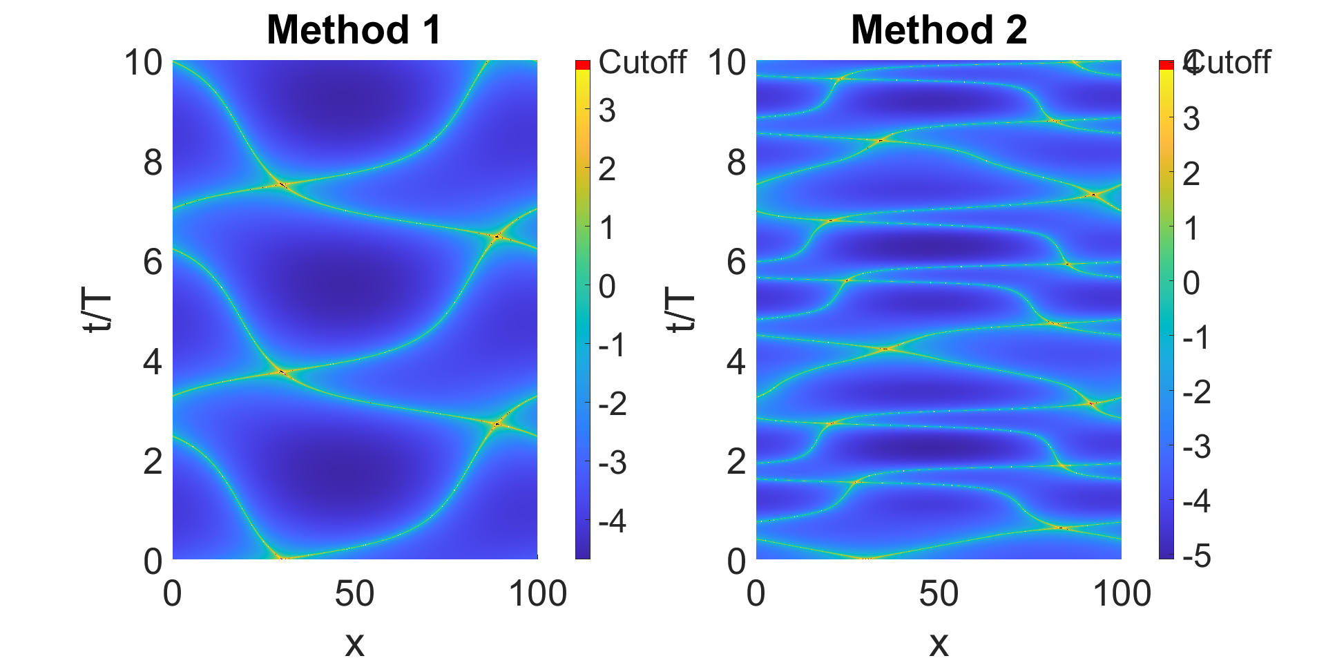
Comparisons between methods are all shown for the same value of since this value has no particular effect when comparing the two results. The consequence of different values of is discussed briefly in the end of this section. Figure 3 shows a comparison between the two methods in the non-heating phase. It might not be clear from the figure that the two methods agree on stroboscopic times even though this is, of course, the case. Instead, the figure illustrates that the two methods disagree in between real times where method 2 takes the micro-motion of the quasi-particles into account. It should be mentioned that any other choice of branch is even worse in comparison as appears from figure 2, which has the same conditions. That branch 0 is the best choice will reappear in several later figures, but the reason is unknown.
There are similarities between the two methods though. Both methods have two trajectories of the quasi-particles. These are the two lines of maxima55 5 These lines are where the function diverges as mentioned earlier. Divergence only occurs exactly on the lines, which means the finite number of points actually plotted are finite. that appear in both cases such that one quasi-particle is moving to the left while another is moving to the right. Notice that the quasi-particles move through the boundaries, which is possible because we chose periodic boundary conditions for the conformal two-point function. These two effects are generic in periodic Floquet CFT with the sine-square deformation66 6 One of the effects of SSD is that the ground states of the original and deformed Hamiltonian agree, if periodic boundary conditions of the original (not the deformed) system are assumedKatsura 2012..
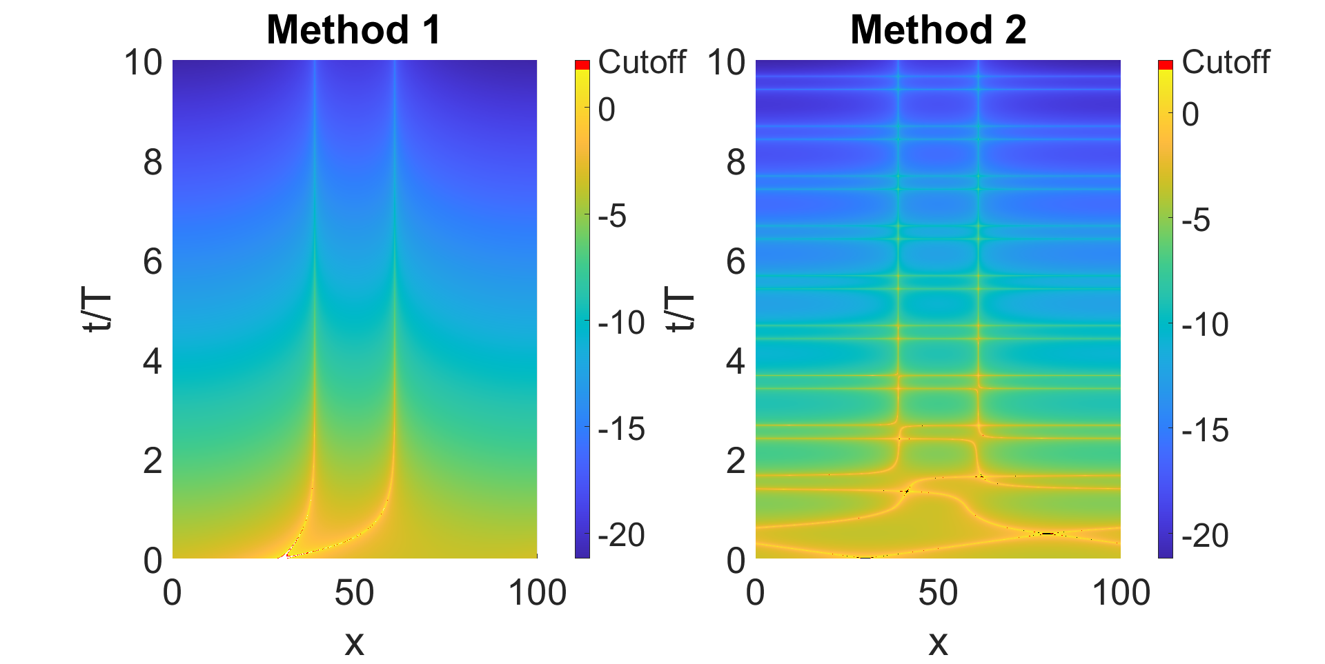
A more interesting comparison occurs in the heating phase illustrated in figure 4. Ignoring the ’’horizontal’’ lines77 7 These almost horizontal lines are a consequence of the -driving. We will later see that method 1 seems to catch the effects of poorly while the effects of are captured quite well. of method 2, the two methods actually agree quite well. In Lapierre et al. 2020a, the trajectories of the quasi-particles as described by method 1 (stroboscopic extrapolation) was shown to follow light-like geodesics in a 2-dimensional Schwarzschild-metric. The light-like geodesic is expected if any since conformal field theories are massless. That is, the quasi-particle trajectories converge towards two points which act approximately like black holes. This will be discussed later. However, when applying method 2 (including micro-motion) convergence does not happen. Instead, the quasi-particles slows down when approaching the points of convergence and speed up when leaving them88 8 The trajectory going to the left is only affected by the right point of stroboscopic convergence and similarly for the other line.. This means that the physical interpretation of the convergence points has turned from attraction to repulsion. It also means that the black hole interpretation is not adequate when including the real time micro-motion of the quasi-particles, even though the relation to black holes still exists at all stroboscopic times.
The ”strength” and ”range” of the repulsion is reflected in how fast the quasi-particle trajectories slow down and accelerate around the points. It can be seen that the ”strength” seems to increase with time while the ”range” is decreasing since the deceleration and acceleration become rapidly more intense with time and happens in a smaller region (the spatial region could also be smaller because the line is moving faster). Remember, that the slope of a trajectory is the inverse of the quasi-particles speed. Thus, if the slope changes mostly within a small time interval, the quasi-particle acceleration must be large, and if the slope changes mostly within a small spatial interval, the range must be short. Note, that these are qualitative observations only and that the idea of strength and range is at most a convenient picture to keep in mind.
It is important to investigate if method 2 really is the correct method. Numerical simulations have already been made in other articles confirming the predictions of method 1 (one such simulation of a spin chain was made in Lapierre et al. 2020a). Interestingly, there are regimes where the two methods agree to high accuracy, and the simulations have been carried out in this regime in Lapierre et al. 2020a. An example can be seen in figure 5. It is worth finding the regimes in which method 1 is a good approximation for three reasons. Firstly, the underlying and yet unknown explanation might help discover new phenomena or describe the system better.
Secondly, method 1 is simpler analytically, especially since method 2 has to be split into two different cases to carry out the calculations. Thirdly, if any future simulations are to be carried out distinguishing between the two methods, this simulation must be carried out in the right regime.
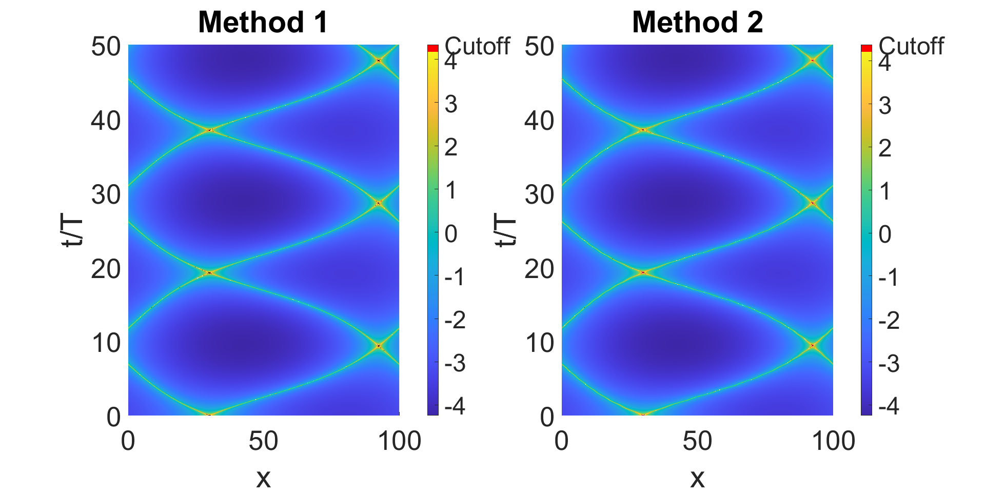
It appears that two criteria need to be satisfied for the methods to approximately agree. Firstly, the period has to be small compared to , meaning that the -driving happens in short intervals99 9 Though it can still make up most of the total driving time. In figure 5 the driving of lasts 50% of the entire driving. . For instance, this is the case in figure 5 since . It is clear why this is the case. When and are small (the high frequency regime), there is little difference between the stroboscopic dynamics and the real-time dynamics since the time difference, , between stroboscopic points becomes small. When becomes small enough, so that is comparable with the resolution of the real-time parameter, the two methods produce identical results. It is clear from the phase diagram in figure 1 that the high-frequency regime is non-heating. However, heating phase dynamics can be obtained in this regime by changing the sign of the uniform Hamiltonian . It also seems to be important that the driving is ”well within” the non-heating phase, which means that cannot be too large so it comes close to the critical line in figure 1, even though it can still be large. This indicates that method 1 is good at describing time evolution by , but not the evolution governed by . If this is true, the same argument as before applies here as well since no considerable differences between the two methods have time to develop during the short driving by , and no or at least very small changes occur during the -driving. However, when the system approaches or even enters the heating regime, very rapid changes take place over time. Now, remember the term ”small” is compared to the time-scale of the system, which means that ” has to be small” is a very restrictive constraint in these circumstances. This would explain why in the bottom of figure 6 can no longer be regarded as small enough for method 1 to be a good approximation.
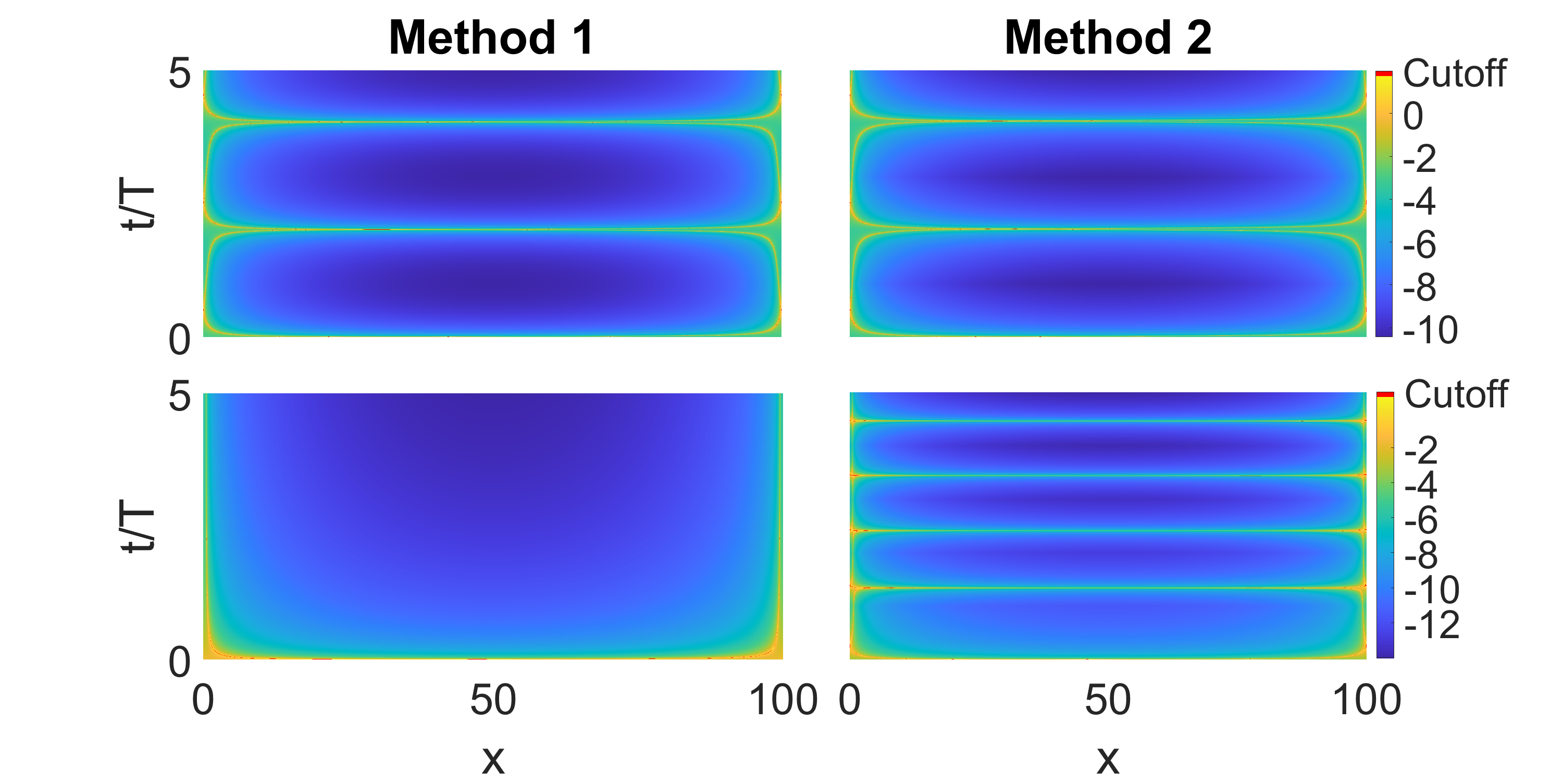
Figure 6 shows some extreme cases and illustrates that method 1 is a good approximation even for very large as long as is small, the driving is in the non-heating phase, and far away from the critical driving. Method 1 is never a good approximation in the heating phase since the ”horizontal” lines appear with method 2 but never with method 1. Interestingly, in the heating phase, is real and the entire problem about branches does therefore not exist here. All the terms ”well within” and ”far away” cannot be stated more precisely since the exact reasons for the similarities are not yet understood.
The fact that has to be small indicates that method 1 is bad at modelling -driving. For , the expression for the two-point function is simple since for such times no actual driving has been introduced. The exact analytical result for is
| (21) | ||||
This expression gives the quasi-particle trajectories:
| (22) |
This explains why the period, when the system is described by , is exactly . The expression is of course more complicated after more periods of driving, but this fact seems to be conserved even though the trajectories are no longer straight lines.
The result in this time-span is plotted in figure 7 and illustrates that method 1 completely fails to describe driving by while method 2 yields the correct result.
Lastly, the two figures 8 and 9 illustrates the effect of different initial conditions. That is different values of . The situation is symmetric for . In the non-heating phase, the patterns are the same but simply ”weighted” towards the position . In the heating phase, the vertical lines are at the same position independent on since they have to agree with method 1 in the stroboscopic times. However, the horizontal lines show a greater vertical distance between the two quasi-particles when the distance to the center increases.


The Geometric Interpretation

In Lapierre et al. 2020a, the surprising result that there exists a relation to black hole dynamics in SSD-driven systems in the heating-phase was discovered. However, since the real time motion was found by method 1, this result has to be questioned. The article Lapierre et al. 2020a argues that the coordinates given by equation 14 are isothermal coordinates of an effective manifold on which the light-like geodesics agree with the lines of maxima. That is, the metric is given by:
| (23) |
and the lines of maxima solve the light-like1010 10 Recall, that conformal fields are massless and thus must follow the light-like geodesic if any. equation:
| (24) |
This idea can be generalized to agree with method 2 simply by taking the metric as:
| (25) |
where is given by equation 19. The equations of motion, and thus the light-like curves, are of course different. In fact, in this case, they correspond to the result obtained by method 2 showing that the geometrical argument used in Lapierre et al. 2020a still works. A numerical simulation is shown in figure 10 and compared to the two-point function in the heating-phase. The equations are way more complicated, however, and are therefore no longer dealt with analytically, contrary to the equations obtained when using method 1.
This is another example of why method 1 still has benefits, although it does not describe the real-time correctly. It also demonstrates how some ideas applied to method 1 still works when applied to method 2.
Of course, the interpretation of real-time motion is no longer that of black holes. But the real-time motion can be stroboscopically interpreted as black hole motion close to the critical points. It is interesting that this interpretation of black holes somehow emerges in the very complex real-time motion, but only at the end of each driving cycle.
It should be mentioned that the current differential equations are very challenging to work with, even numerically. Since the solutions give the trajectories of the quasi-particles an easier way to find them is to find the two-point function (which has the extremely rare benefit of having a known analytical solution) and then simply tracking the trajectories. This also has the consequence that no numerical uncertainty will add up for long time simulations and that the duration of the simulation is unaffected by the desired time span.
Conclusions
Sine-square deformed driven conformal field theories have received much attention recently, but the results have only been calculated up to stroboscopic times, while the full real-time results have merely been implied as an extrapolation thereof. We have found that extrapolation to real times must be done with great care to obtain reliable results. We present an exact method that applies for all times that solves the issue with extrapolation. Though the original extrapolation to real times is not generally reliable, there exists regimes in which it is a good approximation. We have shown that the limit where and is small enough to stay well within the non-heating phase, shows the same behavior in both cases. We argue that this result originates from the fact that the old extrapolation from stroboscopic times accounts poorly for the dynamics of .
Furthermore, as we have discussed, the proposed relationship between SSD conformal Floquet dynamics and the geodesic of a particular black hole dynamics Lapierre et al. 2020a holds only for stroboscopic times, though the geometrical interpretation still works for the new method presented here. The new geodesic equations are too complicated and we have not found analytical solutions, even in appropriate limits. We have made a numerical simulation of the new geodetic motion and compared it to the new two-point function, and our results show excellent agreement between the two approaches. We thus conclude that while the geometric indeed displays the hallmark of a curved space-time, it is not a simple matter to characterize the features of this spacetime. This is an interesting question for future research.
Acknowledgements.
We would like to thank Bastien Lapierre and Ramasubramanian Chitra for looking through our manuscript and for giving us their useful comments.References
- Kitagawa et al. (2010) Takuya Kitagawa, Erez Berg, Mark Rudner, and Eugene Demler, “Topological characterization of periodically driven quantum systems,” Physical Review B 82, 235114 (2010).
- Jiang et al. (2011) Liang Jiang, Takuya Kitagawa, Jason Alicea, AR Akhmerov, David Pekker, Gil Refael, J Ignacio Cirac, Eugene Demler, Mikhail D Lukin, and Peter Zoller, “Majorana fermions in equilibrium and in driven cold-atom quantum wires,” Physical review letters 106, 220402 (2011).
- Rudner et al. (2013) Mark S Rudner, Netanel H Lindner, Erez Berg, and Michael Levin, “Anomalous edge states and the bulk-edge correspondence for periodically driven two-dimensional systems,” Physical Review X 3, 031005 (2013).
- von Keyserlingk and Sondhi (2016a) Curt W von Keyserlingk and Shivaji L Sondhi, “Phase structure of one-dimensional interacting floquet systems. i. abelian symmetry-protected topological phases,” Physical Review B 93, 245145 (2016a).
- Else and Nayak (2016) Dominic V Else and Chetan Nayak, “Classification of topological phases in periodically driven interacting systems,” Physical Review B 93, 201103 (2016).
- Potter et al. (2016) Andrew C Potter, Takahiro Morimoto, and Ashvin Vishwanath, “Classification of interacting topological floquet phases in one dimension,” Physical Review X 6, 041001 (2016).
- Roy and Harper (2016) Rahul Roy and Fenner Harper, “Abelian floquet symmetry-protected topological phases in one dimension,” Physical Review B 94, 125105 (2016).
- Po et al. (2016) Hoi Chun Po, Lukasz Fidkowski, Takahiro Morimoto, Andrew C Potter, and Ashvin Vishwanath, “Chiral floquet phases of many-body localized bosons,” Physical Review X 6, 041070 (2016).
- Roy and Harper (2017) Rahul Roy and Fenner Harper, “Periodic table for floquet topological insulators,” Physical Review B 96, 155118 (2017).
- Harper and Roy (2017) Fenner Harper and Rahul Roy, “Floquet topological order in interacting systems of bosons and fermions,” Physical Review Letters 118, 115301 (2017).
- Po et al. (2017) Hoi Chun Po, Lukasz Fidkowski, Ashvin Vishwanath, and Andrew C Potter, “Radical chiral floquet phases in a periodically driven kitaev model and beyond,” Physical Review B 96, 245116 (2017).
- Potirniche et al. (2017) I-D Potirniche, Andrew C Potter, Monika Schleier-Smith, Ashvin Vishwanath, and Norman Y Yao, “Floquet symmetry-protected topological phases in cold-atom systems,” Physical review letters 119, 123601 (2017).
- Morimoto et al. (2017) Takahiro Morimoto, Hoi Chun Po, and Ashvin Vishwanath, “Floquet topological phases protected by time glide symmetry,” Physical Review B 95, 195155 (2017).
- Fidkowski et al. (2019) Lukasz Fidkowski, Hoi Chun Po, Andrew C Potter, and Ashvin Vishwanath, “Interacting invariants for floquet phases of fermions in two dimensions,” Physical Review B 99, 085115 (2019).
- Yang et al. (2020) Zhaoju Yang, Eran Lustig, Yaakov Lumer, and Mordechai Segev, “Photonic floquet topological insulators in a fractal lattice,” Light: Science & Applications 9, 1–7 (2020).
- Wu and An (2020) Hong Wu and Jun-Hong An, “Floquet topological phases of non-hermitian systems,” Physical Review B 102, 041119 (2020).
- Hu et al. (2020) Haiping Hu, Biao Huang, Erhai Zhao, and W Vincent Liu, “Dynamical singularities of floquet higher-order topological insulators,” Physical Review Letters 124, 057001 (2020).
- Rubio-Abadal et al. (2020) Antonio Rubio-Abadal, Matteo Ippoliti, Simon Hollerith, David Wei, Jun Rui, SL Sondhi, Vedika Khemani, Christian Gross, and Immanuel Bloch, “Floquet prethermalization in a bose-hubbard system,” Physical Review X 10, 021044 (2020).
- Khemani et al. (2016) Vedika Khemani, Achilleas Lazarides, Roderich Moessner, and Shivaji L Sondhi, “Phase structure of driven quantum systems,” Physical review letters 116, 250401 (2016).
- Else et al. (2016) Dominic V Else, Bela Bauer, and Chetan Nayak, “Floquet time crystals,” Physical review letters 117, 090402 (2016).
- von Keyserlingk and Sondhi (2016b) Curt W von Keyserlingk and Shivaji L Sondhi, “Phase structure of one-dimensional interacting floquet systems. ii. symmetry-broken phases,” Physical Review B 93, 245146 (2016b).
- Else et al. (2017) Dominic V Else, Bela Bauer, and Chetan Nayak, “Prethermal phases of matter protected by time-translation symmetry,” Physical Review X 7, 011026 (2017).
- Yao et al. (2017) Norman Y Yao, Andrew C Potter, I-D Potirniche, and Ashvin Vishwanath, “Discrete time crystals: rigidity, criticality, and realizations,” Physical review letters 118, 030401 (2017).
- Kozin and Kyriienko (2019) Valerii K Kozin and Oleksandr Kyriienko, “Quantum time crystals from hamiltonians with long-range interactions,” Physical Review Letters 123, 210602 (2019).
- Surace et al. (2019) Federica Maria Surace, Angelo Russomanno, Marcello Dalmonte, Alessandro Silva, Rosario Fazio, and Fernando Iemini, “Floquet time crystals in clock models,” Physical Review B 99, 104303 (2019).
- Yao et al. (2020) Norman Y Yao, Chetan Nayak, Leon Balents, and Michael P Zaletel, “Classical discrete time crystals,” Nature Physics 16, 438–447 (2020).
- Harper et al. (2020) Fenner Harper, Rahul Roy, Mark S Rudner, and SL Sondhi, “Topology and broken symmetry in floquet systems,” Annual Review of Condensed Matter Physics 11, 345–368 (2020).
- Reitter et al. (2017) Martin Reitter, Jakob Näger, Karen Wintersperger, Christoph Sträter, Immanuel Bloch, André Eckardt, and Ulrich Schneider, “Interaction dependent heating and atom loss in a periodically driven optical lattice,” Physical review letters 119, 200402 (2017).
- Zhang et al. (2017) Jiehang Zhang, PW Hess, A Kyprianidis, P Becker, A Lee, J Smith, G Pagano, I-D Potirniche, Andrew C Potter, A Vishwanath, et al., “Observation of a discrete time crystal,” Nature 543, 217–220 (2017).
- Choi et al. (2017) Soonwon Choi, Joonhee Choi, Renate Landig, Georg Kucsko, Hengyun Zhou, Junichi Isoya, Fedor Jelezko, Shinobu Onoda, Hitoshi Sumiya, Vedika Khemani, et al., “Observation of discrete time-crystalline order in a disordered dipolar many-body system,” Nature 543, 221–225 (2017).
- Maczewsky et al. (2017) Lukas J Maczewsky, Julia M Zeuner, Stefan Nolte, and Alexander Szameit, “Observation of photonic anomalous floquet topological insulators,” Nature communications 8, 1–7 (2017).
- Tang et al. (2018) Yijun Tang, Wil Kao, Kuan-Yu Li, Sangwon Seo, Krishnanand Mallayya, Marcos Rigol, Sarang Gopalakrishnan, and Benjamin L Lev, “Thermalization near integrability in a dipolar quantum newton’s cradle,” Physical Review X 8, 021030 (2018).
- Li et al. (2019) Jiaming Li, Andrew K Harter, Ji Liu, Leonardo de Melo, Yogesh N Joglekar, and Le Luo, “Observation of parity-time symmetry breaking transitions in a dissipative floquet system of ultracold atoms,” Nature communications 10, 1–7 (2019).
- Mukherjee and Rechtsman (2020) Sebabrata Mukherjee and Mikael C Rechtsman, “Observation of floquet solitons in a topological bandgap,” Science 368, 856–859 (2020).
- Qualls (19 May 2016) Joshua D. Qualls, “Lectures on conformal field theory,” arXiv:1511.04074v2 , 45–46 (19 May 2016).
- Ginsparg (1988) Paul Ginsparg, “Applied conformal field theory,” (1988).
- Blumenhagen and Plauschinn (2009) Ralph Blumenhagen and Erik Plauschinn, Introduction to Conformal Field Theory With Applications to String theory (Springer, 2009).
- Wen and Wu (21 May 2018) Xueda Wen and Jie-Qiang Wu, “Floquet conformal field theory,” arXiv:1805.00031v2 (21 May 2018).
- Wen and Wu (2018) Xueda Wen and Jie-Qiang Wu, “Quantum dynamics in sine-square deformed conformal field theory: Quench from uniform to nonuniform conformal field theory,” Physical Review B 97, 184309 (2018).
- Gendiar et al. (2009) Andrej Gendiar, Roman Krcmar, and Tomotoshi Nishino, “Spherical deformation for one-dimensional quantum systems,” Progress of Theoretical Physics 122, 953–967 (2009).
- Hikihara and Nishino (2011) Toshiya Hikihara and Tomotoshi Nishino, “Connecting distant ends of one-dimensional critical systems by a sine-square deformation,” Physical Review B 83, 060414 (2011).
- Gendiar et al. (2011) A Gendiar, M Daniška, Y Lee, and T Nishino, “Suppression of finite-size effects in one-dimensional correlated systems,” Physical Review A 83, 052118 (2011).
- Shibata and Hotta (2011) Naokazu Shibata and Chisa Hotta, “Boundary effects in the density-matrix renormalization group calculation,” Physical Review B 84, 115116 (2011).
- Katsura (2011) Hosho Katsura, “Exact ground state of the sine-square deformed xy spin chain,” Journal of Physics A: Mathematical and Theoretical 44, 252001 (2011).
- Maruyama et al. (2011) Isao Maruyama, Hosho Katsura, and Toshiya Hikihara, “Sine-square deformation of free fermion systems in one and higher dimensions,” Physical Review B 84, 165132 (2011).
- Katsura (2012) Hosho Katsura, “Sine-square deformation of solvable spin chains and conformal field theories,” Journal of Physics A: Mathematical and Theoretical 45, 115003 (2012).
- Ishibashi and Tada (2015) Nobuyuki Ishibashi and Tsukasa Tada, “Infinite circumference limit of conformal field theory,” Journal of Physics A: Mathematical and Theoretical 48, 315402 (2015).
- Ishibashi and Tada (2016) Nobuyuki Ishibashi and Tsukasa Tada, “Dipolar quantization and the infinite circumference limit of two-dimensional conformal field theories,” International Journal of Modern Physics A 31, 1650170 (2016).
- Okunishi (2016) Kouichi Okunishi, “Sine-square deformation and möbius quantization of 2d conformal field theory,” Progress of Theoretical and Experimental Physics 2016, 063A02 (2016).
- Wen et al. (2016) Xueda Wen, Shinsei Ryu, and Andreas WW Ludwig, “Evolution operators in conformal field theories and conformal mappings: Entanglement hamiltonian, the sine-square deformation, and others,” Physical Review B 93, 235119 (2016).
- Tamura and Katsura (2017) Shota Tamura and Hosho Katsura, “Zero-energy states in conformal field theory with sine-square deformation,” Progress of Theoretical and Experimental Physics 2017, 113A01 (2017).
- Tada (2015) Tsukasa Tada, “Sine-square deformation and its relevance to string theory,” Modern Physics Letters A 30, 1550092 (2015).
- Lapierre and Moosavi (2020) Bastian Lapierre and Per Moosavi, “A geometric approach to inhomogeneous floquet systems,” arXiv:2010.11268 (2020).
- Fan et al. (2020a) Ruihua Fan, Yingfei Gu, Ashvin Vishwanath, and Xueda Wen, “Emergent spatial structure and entanglement localization in floquet conformal field theory,” Physical Review X 10, 031036 (2020a).
- Fan et al. (2020b) Ruihua Fan, Yingfei Gu, Ashvin Vishwanath, and Xueda Wen, “Floquet conformal field theory,” Bulletin of the American Physical Society 65 (2020b).
- Han and Wen (2020) Bo Han and Xueda Wen, “Classification of deformed floquet conformal field theories,” arXiv preprint arXiv:2008.01123 (2020).
- Lapierre et al. (2020a) Bastien Lapierre, Kenny Choo, Clément Tauber, Apoorv Tiwari, Titus Neupert, and Ramasubramanian Chitra, “Emergent black hole dynamics in critical floquet systems,” Physical Review Research 2, 023085 (2020a).
- Fan et al. (2020c) Ruihua Fan, Yingfei Gu, Ashvin Vishwanath, and Xueda Wen, “Emergent spatial structure and entanglement localization in floquet conformal field theory,” Physical Review X 10, 031036 (2020c).
- Lapierre et al. (2020b) Bastien Lapierre, Kenny Choo, Apoorv Tiwari, Clément Tauber, Titus Neupert, and Ramasubramanian Chitra, “Fine structure of heating in a quasiperiodically driven critical quantum system,” Physical Review Research 2, 033461 (2020b).