Recursive Importance Sketching for Rank Constrained Least Squares: Algorithms and High-order Convergence

We introduce an easy-to-implement and computationally efficient algorithm, Recursive Importance Sketching for Rank constrained least squares Optimization (RISRO), for solving (1) in this paper. The proposed algorithm is tuning free and has the same per-iteration computational complexity as Alternating Minimization (Jain et al., 2013), as well as comparable complexity to many popular first-order methods such as iterative hard thresholding (Jain et al., 2010) and gradient descent (Tu et al., 2016) when $r\ll p_{1},p_{2},n$. We then illustrate the key idea of RISRO under a general framework of recursive importance sketching. This framework also renders a platform to compare RISRO and several existing algorithms for rank constrained least squares.

Assuming ${\mathcal{A}}$ satisfies the restricted isometry property (RIP), we prove RISRO is local quadratic-linearly convergent in general and quadratically convergent to a stationary point under some extra conditions. Figure 1 provides a numerical example of the performance of RISRO in the noiseless low-rank matrix trace regression (left panel) and phase retrieval (right panel). In both problems, RISRO converges to the underlying parameter quadratically and reaches a highly accurate solution within five iterations.

In addition, we discover a deep connection between RISRO and the Riemannian Gauss-Newton optimization algorithm on fixed rank matrices manifold. The least squares step in RISRO implicitly solves a Fisher Scoring or Riemannian Gauss-Newton equation on the Riemannian optimization of low-rank matrices and the updating rule in RISRO can be seen as a retraction map. With this connection, our theory on RISRO also improves the existing convergence results on the Riemannian Gauss-Newton method for the rank constrained least squares problem.

Next, we further apply RISRO to two prominent problems in machine learning and statistics: low-rank matrix trace regression and phase retrieval. In the noisy low-rank matrix trace regression, we prove the estimation error rate of RISRO converges quadratically to the information-theoretical limit with only a double-logarithmic number of iterations under the Gaussian ensemble design. To the best of our knowledge, RISRO is the first algorithm that provably achieves the minimax rate-optimal estimation error in matrix trace regression with only a double-logarithmic number of iterations, which offers an exponential improvement over the existing results of first-order methods (Jain et al., 2010; Jain et al., 2013; Chen and Wainwright, 2015). We also discover a new “quadratic + one-iteration optimality” phenomenon for RISRO on low-rank matrix recovery (Remark 12). In phase retrieval, where ${\mathcal{A}}$ does not satisfy the RIP condition, we can still establish the local convergence of RISRO given a proper initialization. We also develop RISRO in the matrix completion and robust PCA applications, where the restricted isometry property completely fails. We find RISRO still has similar empirical performance as in the setting where the RIP condition holds.

Finally, we conduct simulation studies to support our theoretical findings and compare RISRO with many existing algorithms. The numerical results show RISRO not only offers faster and more robust convergence but also requires a smaller sample size requirement for low-rank matrix recovery, compared to existing approaches.

This work is related to a range of literature on low-rank matrix recovery, convex/non-convex optimization, and sketching arising from several communities, including optimization, machine learning, statistics, and applied mathematics. We make an attempt to review the related literature without claiming the survey is exhaustive.

One class of the most popular approaches to solve (1) is the nuclear norm minimization (NNM) (3). Many algorithms have been proposed to solve NNM, such as proximal gradient descent (Toh and Yun, 2010), fixed-point continuation (FPC) (Goldfarb and Ma, 2011), and proximal point methods (Jiang et al., 2014). It has been shown that the solution of NNM has desirable properties under proper models, such as matrix trace regression and matrix completion (Cai and Zhang, 2013; Cai and Zhang, 2014; Cai and Zhang, 2015; Candès and Plan, 2011; Recht et al., 2010). In addition to NNM, the max norm minimization is another widely considered convex realization for the rank constrained optimization (Lee et al., 2010; Cai and Zhou, 2013). However, these convex programs are usually computationally intensive to solve, which motivates a line of work on using non-convex approaches. Since Burer and Monteiro, 2003, one of the most popular non-convex methods for solving (1) is to first factor the low-rank matrix ${\mathbf{X}}$ to ${\mathbf{R}}{\mathbf{L}}^{\top}$ with two factor matrices ${\mathbf{R}}\in\mathbb{R}^{p_{1}\times r},{\mathbf{L}}\in\mathbb{R}^{p_{2}\times r}$, then run either gradient descent or alternating minimization on ${\mathbf{R}}$ and ${\mathbf{L}}$ (Candès et al., 2015; Li et al., 2019b; Ma et al., 2019; Park et al., 2018; Sanghavi et al., 2017; Sun and Luo, 2016; Tu et al., 2016; Wang et al., 2017c; Zhao et al., 2015; Zheng and Lafferty, 2015; Tong et al., 2021b). Other methods, such as singular value projection or iterative hard thresholding (Goldfarb and Ma, 2011; Jain et al., 2010; Tanner and Wei, 2013), Grassmann manifold optimization (Boumal and Absil, 2011; Keshavan et al., 2009), Riemannian manifold optimization (Huang and Hand, 2018; Meyer et al., 2011; Mishra et al., 2014; Vandereycken, 2013; Wei et al., 2016) have also been proposed and studied. We refer readers to the recent survey paper Chi et al., 2019 for a comprehensive overview of existing literature on convex and non-convex approaches on solving (1). Most of the convergence analyses in the literature were conducted under certain statistical models (e.g., noisy/noiseless matrix trace regression, matrix completion, and phase retrieval) and the goal was to recover the underlying parameter matrix. Here, we study (1) from both an optimization perspective (how the algorithm converges to a stationary point) and a statistical perspective (how the iterates estimate the underlying true parameter). These two perspectives overlap in the noiseless settings as the parameter becomes a stationary point then, while disjoint in the more general noisy settings.

There are a few recent attempts in connecting the geometric structures of different approaches (Ha et al., 2020; Li et al., 2019a), and the landscape of problem (1) has also been studied in various settings (Bhojanapalli et al., 2016; Ge et al., 2017; Uschmajew and Vandereycken, 2020; Zhang et al., 2019; Zhu et al., 2018).

Our work is also related to the idea of sketching in numerical linear algebra. Performing sketching to speed up the computation via dimension reduction has been explored extensively in recent years (Mahoney, 2011; Woodruff, 2014). Sketching methods have been applied to solve a number of problems including but not limited to matrix approximation (Song et al., 2017; Zheng et al., 2012; Drineas et al., 2012), linear regression (Clarkson and Woodruff, 2017; Dobriban and Liu, 2019; Pilanci and Wainwright, 2016; Raskutti and Mahoney, 2016), ridge regression (Wang et al., 2017b), etc. In most of the sketching literature, the sketching matrices are randomly constructed (Mahoney, 2011; Woodruff, 2014). Randomized sketching matrices are easy to generate and require little storage for sparse sketching. However, randomized sketching can be suboptimal in statistical settings (Raskutti and Mahoney, 2016). To overcome this, Zhang et al., 2020 introduced an idea of importance sketching in the context of low-rank tensor regression. In contrast to the randomized sketching, importance sketching matrices are constructed deterministically with the supervision of the data and are shown capable of achieving better statistical efficiency. However, the method developed is Zhang et al., 2020 is essentially a “one-time” importance sketching, which yield a sub-optimal outcome when the noise level is small or moderate. This paper proposes a more powerful recursive importance sketching algorithm that iteratively refines the sketching matrices. We also provide a comprehensive convergence analysis for the proposed algorithm without the sample-splitting assumption used in Zhang et al., 2020; our theory demonstrates the optimality of the proposed algorithm at all different noise levels and advantages over other algorithms for the rank constrained least squares problem.

The rest of this article is organized as follows. After a brief introduction of notation in Section 1.4, we present our main algorithm RISRO with an interpretation from the recursive importance sketching perspective in Section 2. The theoretical results of RISRO are given in Section 3. In Section 4, we present another interpretation for RISRO from Riemannian manifold optimization. The computational complexity of RISRO and its applications to low-rank matrix trace regression and phase retrieval are discussed in Sections 5 and 6, respectively. Numerical studies of RISRO and the comparison with existing algorithms in the literature are presented in Section 7. Conclusion and future work are given in Section 8.

The following notation will be used throughout this article. Upper and lowercase letters (e.g., $A,B,a,b$), lowercase boldface letters (e.g. ${\mathbf{u}},{\mathbf{v}}$), uppercase boldface letters (e.g., ${\mathbf{U}},{\mathbf{V}}$) are used to denote scalars, vectors, matrices, respectively. For any two series of numbers, say $\{a_{n}\}$ and $\{b_{n}\}$, denote $a=O(b)$ if there exists uniform constants $C>0$ such that $a_{n}\leq Cb_{n},\forall n$. For any $a,b\in\mathbb{R}$, let $a\wedge b:=\min\{a,b\},a\vee b=\max\{a,b\}$. For any matrix ${\mathbf{X}}\in\mathbb{R}^{p_{1}\times p_{2}}$ with singular value decomposition $\sum_{i=1}^{p_{1}\land p_{2}}\sigma_{i}({\mathbf{X}}){\mathbf{u}}_{i}{\mathbf{v}}_{i}^{\top}$, where $\sigma_{1}({\mathbf{X}})\geq\sigma_{2}({\mathbf{X}})\geq\cdots\geq\sigma_{p_{1}\wedge p_{2}}({\mathbf{X}})$, let ${\mathbf{X}}_{\max(r)}=\sum_{i=1}^{r}\sigma_{i}({\mathbf{X}}){\mathbf{u}}_{i}{\mathbf{v}}_{i}^{\top}$ be the best rank-$r$ approximation of ${\mathbf{X}}$ and denote $\|{\mathbf{X}}\|_{\rm F}=\sqrt{\sum_{i}\sigma^{2}_{i}({\mathbf{X}})}$ and $\|{\mathbf{X}}\|=\sigma_{1}({\mathbf{X}})$ as the Frobenius norm and spectral norm, respectively. Let ${\rm QR}({\mathbf{X}})$ be the $Q$ part of the QR decomposition outcome of ${\mathbf{X}}$. ${\rm vec}({\mathbf{X}})\in\mathbb{R}^{p_{1}p_{2}}$ represents the vectorization of ${\mathbf{X}}$ by its columns. In addition, ${\mathbf{I}}_{r}$ is the $r$-by-$r$ identity matrix. Let $\mathbb{O}_{p,r}=\{{\mathbf{U}}:{\mathbf{U}}^{\top}{\mathbf{U}}={\mathbf{I}}_{r}\}$ be the set of all $p$-by-$r$ matrices with orthonormal columns. For any ${\mathbf{U}}\in\mathbb{O}_{p,r}$, $P_{{\mathbf{U}}}={\mathbf{U}}{\mathbf{U}}^{\top}$ represents the orthogonal projector onto the column space of ${\mathbf{U}}$; we also note ${\mathbf{U}}_{\perp}\in\mathbb{O}_{p,p-r}$ as the orthonormal complement of ${\mathbf{U}}$. We use bracket subscripts to denote sub-matrices. For example, ${\mathbf{X}}_{[i_{1},i_{2}]}$ is the entry of ${\mathbf{X}}$ on the $i_{1}$-th row and $i_{2}$-th column; ${\mathbf{X}}_{[(r+1):p_{1},:]}$ contains the $(r+1)$-th to the $p_{1}$-th rows of ${\mathbf{X}}$. For any matrix ${\mathbf{X}}$, we use ${\mathbf{X}}^{\dagger}$ to denote its Moore-Penrose inverse. For matrices ${\mathbf{U}}\in\mathbb{R}^{p_{1}\times p_{2}},{\mathbf{V}}\in\mathbb{R}^{m_{1}\times m_{2}}$, let

be their Kronecker product. Finally, for any given linear operator ${\cal L}$, we use ${\mathcal{L}}^{*}$ to denote its adjoint, and use ${\rm Ran}({\mathcal{L}})$ to denote its range space.

In each iteration $t=1,2,\ldots$, RISRO includes three steps.

• Step 1

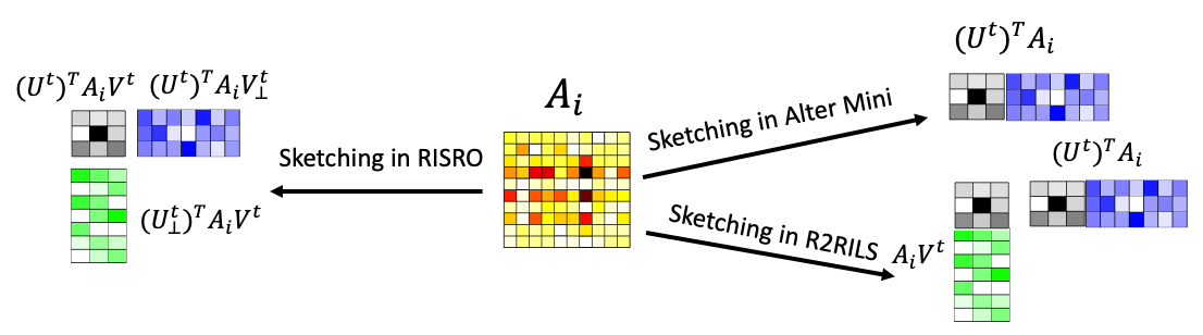
  We sketch each ${\mathbf{A}}_{i}$ ($i=1,\ldots,n$) onto the subspace spanned by $[{\mathbf{U}}^{t}\otimes{\mathbf{V}}^{t},{\mathbf{U}}_{\perp}^{t}\otimes{\mathbf{V}}^{t},{\mathbf{U}}^{t}\otimes{\mathbf{V}}_{\perp}^{t}]$, where ${\mathbf{U}}^{t}$ and ${\mathbf{V}}^{t}$ span the column and row subspaces of ${\mathbf{X}}^{t}$, respectively. This yields the sketched importance covariates ${\mathbf{U}}^{t\top}{\mathbf{A}}_{i}{\mathbf{V}}^{t},{\mathbf{U}}^{t\top}_{\perp}{\mathbf{A}}_{i}{\mathbf{V}}^{t},{\mathbf{U}}^{t\top}{\mathbf{A}}_{i}{\mathbf{V}}^{t}_{\perp}$. See Figure 2 left panel for an illustration of the sketching scheme of RISRO. Then we construct the covariates maps ${\mathcal{A}}_{B}:\mathbb{R}^{r\times r}\to\mathbb{R}^{n}$, ${\mathcal{A}}_{D_{1}}:\mathbb{R}^{(p_{1}-r)\times r}\to\mathbb{R}^{n}$ and ${\mathcal{A}}_{D_{2}}:\mathbb{R}^{r\times(p_{2}-r)}\to\mathbb{R}^{n}$: for matrix “$\cdot$”, let

  $$[{\mathcal{A}}_{B}(\cdot)]_{i}=\langle\cdot,{\mathbf{U}}^{t\top}{\mathbf{A}}_{i}{\mathbf{V}}^{t}\rangle,\quad[{\mathcal{A}}_{D_{1}}(\cdot)]_{i}=\langle\cdot,{\mathbf{U}}_{\perp}^{t\top}{\mathbf{A}}_{i}{\mathbf{V}}^{t}\rangle,\quad[{\mathcal{A}}_{D_{2}}(\cdot)]_{i}=\langle\cdot,{\mathbf{U}}^{t\top}{\mathbf{A}}_{i}{\mathbf{V}}_{\perp}^{t}\rangle,\quad i=1,\ldots,n.$$

  (4)

• Step 2

  We solve a dimension reduced least squares problem (5) (provided in the box of Algorithm 1) where the number of parameters is reduced to $(p_{1}+p_{2}-r)r$ while the sample size remains $n$.

• Step 3

  We update the sketching matrices ${\mathbf{U}}^{t+1},{\mathbf{V}}^{t+1}$ and ${\mathbf{X}}^{t+1}$ in Steps  6 and 7. By construction, ${\mathbf{U}}^{t+1},{\mathbf{V}}^{t+1}$ contain both the column and row spans of ${\mathbf{X}}^{t+1}$.

We give a high-level explanation of RISRO through a decomposition of ${\mathbf{y}}_{i}$. Suppose ${\mathbf{y}}_{i}=\langle{\mathbf{A}}_{i},\widebar{{\mathbf{X}}}\rangle+\widebar{{\boldsymbol{\epsilon}}}_{i}$ where $\widebar{{\mathbf{X}}}$ is a rank $r$ target matrix with singular value decomposition $\widebar{{\mathbf{U}}}\widebar{{\boldsymbol{\Sigma}}}\widebar{{\mathbf{V}}}^{\top}$ with $\widebar{\mathbf{U}}\in\mathbb{O}_{p_{1},r}$, $\widebar{\boldsymbol{\Sigma}}\in\mathbb{R}^{r\times r}$ and $\widebar{\mathbf{V}}\in\mathbb{O}_{p_{2},r}$. Then

Here, ${\boldsymbol{\epsilon}}^{t}:={\mathcal{A}}(P_{{\mathbf{U}}^{t}_{\perp}}\widebar{{\mathbf{X}}}P_{{\mathbf{V}}^{t}_{\perp}})+\widebar{{\boldsymbol{\epsilon}}}\in\mathbb{R}^{n}$ can be seen as the residual of the new regression model (6), and ${\mathbf{U}}^{t\top}{\mathbf{A}}_{i}{\mathbf{V}}^{t},{\mathbf{U}}^{t\top}_{\perp}{\mathbf{A}}_{i}{\mathbf{V}}^{t},{\mathbf{U}}^{t\top}{\mathbf{A}}_{i}{\mathbf{V}}^{t}_{\perp}$ are exactly the importance covariates constructed in (4). Let

If ${\boldsymbol{\epsilon}}^{t}=0$, we have $(\widetilde{{\mathbf{B}}}^{t},\widetilde{{\mathbf{D}}}_{1}^{t},\widetilde{{\mathbf{D}}}_{2}^{t})$ is a solution of the least squares in (5). Hence, we could set ${\mathbf{B}}^{t+1}=\widetilde{{\mathbf{B}}}^{t},{\mathbf{D}}_{1}^{t+1}=\widetilde{{\mathbf{D}}}_{1}^{t},{\mathbf{D}}_{2}^{t+1}=\widetilde{{\mathbf{D}}}_{2}^{t}$ and thus ${\mathbf{X}}_{U}^{t+1}=\widebar{{\mathbf{X}}}{\mathbf{V}}^{t},{\mathbf{X}}_{V}^{t+1}=\widebar{{\mathbf{X}}}^{\top}{\mathbf{U}}^{t}$. Furthermore, if ${\mathbf{B}}^{t+1}$ is invertible, then it holds that

which means $\widebar{{\mathbf{X}}}$ can be exactly recovered by one iteration of RISRO.

In general, ${\boldsymbol{\epsilon}}^{t}\neq 0$. When the column spans of ${\mathbf{U}}^{t},{\mathbf{V}}^{t}$ well approximate the ones of $\widebar{{\mathbf{U}}},\widebar{{\mathbf{V}}}$, i.e., the column and row subspaces that the target parameter $\widebar{{\mathbf{X}}}$ lie on, we expect ${\mathbf{U}}^{t\top}_{\perp}\widebar{{\mathbf{X}}}{\mathbf{V}}^{t}_{\perp}$ and ${\boldsymbol{\epsilon}}^{t}_{i}=\langle{\mathbf{U}}_{\perp}^{t\top}{\mathbf{A}}_{i}{\mathbf{V}}_{\perp}^{t},{\mathbf{U}}_{\perp}^{t\top}\widebar{{\mathbf{X}}}{\mathbf{V}}_{\perp}^{t}\rangle+\widebar{{\boldsymbol{\epsilon}}}_{i}$ to have a small amplitude, then ${\mathbf{B}}^{t+1},{\mathbf{D}}_{1}^{t+1},{\mathbf{D}}_{2}^{t+1}$, the outcome of the least squares problem (5), can well approximate $\widetilde{{\mathbf{B}}}^{t},\widetilde{{\mathbf{D}}}_{1}^{t},\widetilde{{\mathbf{D}}}_{2}^{t}$. In Lemma 1, we give a precise characterization for this approximation. Before that, let us introduce a convenient notation so that (5) can be written in a more compact way.

Define the linear operator ${\cal L}_{t}$ as

and it is easy to compute its adjoint ${\cal L}^{*}_{t}:{\mathbf{M}}\in\mathbb{R}^{p_{1}\times p_{2}}\to\begin{bmatrix}{\mathbf{U}}^{t\top}{\mathbf{M}}{\mathbf{V}}^{t}&{\mathbf{U}}^{t\top}{\mathbf{M}}{\mathbf{V}}^{t}_{\perp}\\ ({\mathbf{U}}^{t}_{\perp})^{\top}{\mathbf{M}}{\mathbf{V}}^{t}&{\mathbf{0}}\end{bmatrix}$. Then, the least squares problem in (5) can be written as

In view of Lemma 1, the approximation errors of ${\mathbf{B}}^{t+1},{\mathbf{D}}_{1}^{t+1},{\mathbf{D}}_{2}^{t+1}$ to $\widetilde{{\mathbf{B}}}^{t},\widetilde{{\mathbf{D}}}_{1}^{t},\widetilde{{\mathbf{D}}}_{2}^{t}$ are driven by the least squares residual $\|({\mathcal{L}}_{t}^{*}{\mathcal{A}}^{*}{\mathcal{A}}{\mathcal{L}}_{t})^{-1}{\mathcal{L}}_{t}^{*}{\mathcal{A}}^{*}{\boldsymbol{\epsilon}}^{t}\|_{\rm F}^{2}$. This fact plays a key role in the proof for the high-order convergence theory of RISRO, see later in Remark 7.

In addition to RISRO, several classic algorithms for rank constrained least squares can be interpreted from the recursive importance sketching perspective. Through the lens of the sketching, RISRO exhibits advantages over these existing algorithms.

We first focus on Alternating Minimization (Alter Mini) proposed and studied in Hardt, 2014; Jain et al., 2013; Zhao et al., 2015. Suppose ${\mathbf{U}}^{t}$ is the left singular vectors of ${\mathbf{X}}^{t}$, the outcome of the $t$-th iteration, Alter Mini solves the following least squares problems to update ${\mathbf{U}}$ and ${\mathbf{V}}$,

Then, Alter Mini essentially solves least squares problems with sketched covariates ${\mathbf{U}}^{t\top}{\mathbf{A}}_{i},{\mathbf{A}}_{i}{\mathbf{V}}^{t+1}$ to update $\widecheck{{\mathbf{V}}}^{t+1},\widecheck{{\mathbf{U}}}^{t+1}$ alternatively and iteratively. The number of parameters of the least squares in (13) are $rp_{2}$ and $rp_{1}$ as opposed to $p_{1}p_{2}$, the number of parameters in the original least squares problem. See Figure 2 upper right panel for an illustration of the sketching scheme in Alter Mini. Consider the following decomposition of ${\mathbf{y}}_{i}$,

where $\widecheck{{\boldsymbol{\epsilon}}}^{t}:={\mathcal{A}}(P_{{\mathbf{U}}^{t}_{\perp}}\widebar{{\mathbf{X}}})+\bar{\boldsymbol{\epsilon}}\in\mathbb{R}^{n}$. Define $\widecheck{{\mathbf{A}}}^{t}\in\mathbb{R}^{n\times p_{2}r}$ with $\widecheck{{\mathbf{A}}}_{[i,:]}={\rm vec}({\mathbf{U}}^{t\top}{\mathbf{A}}_{i})$. Similar to how Lemma 1 is proved, we can show $\|\widecheck{{\mathbf{V}}}^{t+1\top}-{\mathbf{U}}^{t\top}\widebar{{\mathbf{X}}}\|^{2}_{\rm F}=\|(\widecheck{{\mathbf{A}}}^{t\top}\widecheck{{\mathbf{A}}}^{t})^{-1}\widecheck{{\mathbf{A}}}^{t\top}\widecheck{{\boldsymbol{\epsilon}}}^{t}\|_{2}^{2},$ which implies the approximation error of ${\mathbf{V}}^{t+1}={\rm QR}(\widecheck{{\mathbf{V}}}^{t+1})$ (i.e., the outcome of one iteration Alter Mini) to $\widebar{{\mathbf{V}}}$ (i.e., true row span of the target matrix $\widebar{{\mathbf{X}}}$) is driven by $\widecheck{{\boldsymbol{\epsilon}}}^{t}={\mathcal{A}}(P_{{\mathbf{U}}^{t}_{\perp}}\widebar{{\mathbf{X}}})+\bar{\boldsymbol{\epsilon}}$, i.e., the residual of least squares problem (14). Recall for RISRO, Lemma 1 shows the approximation error of ${\mathbf{V}}^{t+1}$ is driven by ${\boldsymbol{\epsilon}}^{t}={\mathcal{A}}(P_{{\mathbf{U}}^{t}_{\perp}}\widebar{{\mathbf{X}}}P_{{\mathbf{V}}^{t}_{\perp}})+\bar{\boldsymbol{\epsilon}}$. Since $\|P_{{\mathbf{U}}_{\perp}^{t}}\widebar{{\mathbf{X}}}P_{{\mathbf{V}}_{\perp}^{t}}\|_{\rm F}\leq\|P_{{\mathbf{U}}_{\perp}^{t}}\widebar{{\mathbf{X}}}\|_{\rm F}$, the approximation error in per iteration of RISRO can be smaller than the one of Alter Mini. Such a difference between RISRO and Alter Mini is due to the following fact: in Alter Mini, the sketching captures the importance covariates correspond to only the row (or column) span of ${\mathbf{X}}^{t}$ in updating ${\mathbf{V}}^{t+1}$ (or ${\mathbf{U}}^{t+1}$), while the importance sketching of RISRO in (4) catches the importance covariates from both the row span and column span of ${\mathbf{X}}^{t}$. As a consequence, Alter Mini iterations yield first-order convergence while RISRO iterations render high-order convergence as will be established in Section 3.

Another example is the rank $2r$ iterative least squares (R2RILS) proposed in Bauch et al., 2021 for solving ill-conditioned matrix completion problems. In particular, at the $t$-th iteration, Step 1 of R2RILS solves the following least squares problem

where $\Omega$ is the set of index pairs of the observed entries. In the matrix completion setting, it turns out the following equivalence holds (proof given in Appendix)

where ${\mathbf{A}}^{ij}\in\mathbb{R}^{p_{1}\times p_{2}}$ is the special covariate in matrix completion satisfying $({\mathbf{A}}^{ij})_{[k,l]}=1$ if $(i,j)=(k,l)$ and $({\mathbf{A}}^{ij})_{[k,l]}=0$ otherwise. This equivalence reveals that the least squares step (15) in R2RILS can be seen as an implicit sketched least squares problem similar to (5) and (13) with covariates ${\mathbf{U}}^{t\top}{\mathbf{A}}^{ij}$ and ${\mathbf{A}}^{ij}{\mathbf{V}}^{t}$ for $(i,j)\in\Omega$.

We give a pictorial illustration for the sketching interpretation of R2RILS on the bottom right part of Figure 2. Different from the sketching in RISRO, R2RILS incorporates the core sketch ${\mathbf{U}}^{t\top}{\mathbf{A}}_{i}{\mathbf{V}}^{t}$ twice, which results in the rank deficiency in the least squares problem (15) and brings difficulties in both implementation and theoretical analysis. RISRO overcomes this issue by performing a better-designed sketching and covers more general low-rank matrix recovery settings than R2RILS. With the new sketching scheme, we are able to give a new and solid theory for RISRO with high-order convergence.

References

• Absil et al., (2008) Absil, P.-A., Mahony, R., and Sepulchre, R. (2008). Optimization Algorithms on Matrix Manifolds. Princeton University Press.
• Absil and Malick, (2012) Absil, P.-A. and Malick, J. (2012). Projection-like retractions on matrix manifolds. SIAM Journal on Optimization, 22(1):135–158.
• Ahmed et al., (2013) Ahmed, A., Recht, B., and Romberg, J. (2013). Blind deconvolution using convex programming. IEEE Transactions on Information Theory, 60(3):1711–1732.
• Bauch et al., (2021) Bauch, J., Nadler, B., and Zilber, P. (2021). Rank 2​r2r iterative least squares: efficient recovery of ill-conditioned low rank matrices from few entries. SIAM Journal on Mathematics of Data Science, 3(1):439–465.
• Bhojanapalli et al., (2016) Bhojanapalli, S., Neyshabur, B., and Srebro, N. (2016). Global optimality of local search for low rank matrix recovery. In Advances in Neural Information Processing Systems, pages 3873–3881.
• Boumal and Absil, (2011) Boumal, N. and Absil, P.-A. (2011). Rtrmc: A Riemannian trust-region method for low-rank matrix completion. In Advances in Neural Information Processing Systems, pages 406–414.
• Breiding and Vannieuwenhoven, (2018) Breiding, P. and Vannieuwenhoven, N. (2018). Convergence analysis of Riemannian Gauss–Newton methods and its connection with the geometric condition number. Applied Mathematics Letters, 78:42–50.
• Burer and Monteiro, (2003) Burer, S. and Monteiro, R. D. (2003). A nonlinear programming algorithm for solving semidefinite programs via low-rank factorization. Mathematical Programming, 95(2):329–357.
• Burke, (1985) Burke, J. V. (1985). Descent methods for composite nondifferentiable optimization problems. Mathematical Programming, 33(3):260–279.
• Cai and Zhang, (2013) Cai, T. T. and Zhang, A. (2013). Sharp RIP bound for sparse signal and low-rank matrix recovery. Applied and Computational Harmonic Analysis, 35(1):74–93.
• Cai and Zhang, (2014) Cai, T. T. and Zhang, A. (2014). Sparse representation of a polytope and recovery of sparse signals and low-rank matrices. IEEE Transactions on Information Theory, 60(1):122–132.
• Cai and Zhang, (2015) Cai, T. T. and Zhang, A. (2015). ROP: Matrix recovery via rank-one projections. The Annals of Statistics, 43(1):102–138.
• Cai and Zhang, (2018) Cai, T. T. and Zhang, A. (2018). Rate-optimal perturbation bounds for singular subspaces with applications to high-dimensional statistics. The Annals of Statistics, 46(1):60–89.
• Cai and Zhou, (2013) Cai, T. T. and Zhou, W.-X. (2013). A max-norm constrained minimization approach to 1-bit matrix completion. The Journal of Machine Learning Research, 14(1):3619–3647.
• Candès, (2008) Candès, E. J. (2008). The restricted isometry property and its implications for compressed sensing. Comptes Rendus Mathematique, 346(9-10):589–592.
• Candès et al., (2011) Candès, E. J., Li, X., Ma, Y., and Wright, J. (2011). Robust principal component analysis? Journal of the ACM (JACM), 58(3):11.
• Candès et al., (2015) Candès, E. J., Li, X., and Soltanolkotabi, M. (2015). Phase retrieval via Wirtinger flow: Theory and algorithms. IEEE Transactions on Information Theory, 61(4):1985–2007.
• Candès and Plan, (2011) Candès, E. J. and Plan, Y. (2011). Tight oracle inequalities for low-rank matrix recovery from a minimal number of noisy random measurements. IEEE Transactions on Information Theory, 57(4):2342–2359.
• Candès et al., (2013) Candès, E. J., Strohmer, T., and Voroninski, V. (2013). Phaselift: Exact and stable signal recovery from magnitude measurements via convex programming. Communications on Pure and Applied Mathematics, 66(8):1241–1274.
• Candès and Tao, (2010) Candès, E. J. and Tao, T. (2010). The power of convex relaxation: Near-optimal matrix completion. IEEE Transactions on Information Theory, 56(5):2053–2080.
• Charisopoulos et al., (2021) Charisopoulos, V., Chen, Y., Davis, D., Díaz, M., Ding, L., and Drusvyatskiy, D. (2021). Low-rank matrix recovery with composite optimization: good conditioning and rapid convergence. Foundations of Computational Mathematics, 21(6):1505–1593.
• Chen and Candès, (2017) Chen, Y. and Candès, E. J. (2017). Solving random quadratic systems of equations is nearly as easy as solving linear systems. Communications on Pure and Applied Mathematics, 70(5):822–883.
• Chen et al., (2015) Chen, Y., Chi, Y., and Goldsmith, A. J. (2015). Exact and stable covariance estimation from quadratic sampling via convex programming. IEEE Transactions on Information Theory, 61(7):4034–4059.
• Chen and Wainwright, (2015) Chen, Y. and Wainwright, M. J. (2015). Fast low-rank estimation by projected gradient descent: General statistical and algorithmic guarantees. arXiv preprint arXiv:1509.03025.
• Chi et al., (2019) Chi, Y., Lu, Y. M., and Chen, Y. (2019). Nonconvex optimization meets low-rank matrix factorization: An overview. IEEE Transactions on Signal Processing, 67(20):5239–5269.
• Clarkson and Woodruff, (2017) Clarkson, K. L. and Woodruff, D. P. (2017). Low-rank approximation and regression in input sparsity time. Journal of the ACM (JACM), 63(6):54.
• Davenport and Romberg, (2016) Davenport, M. A. and Romberg, J. (2016). An overview of low-rank matrix recovery from incomplete observations. IEEE Journal of Selected Topics in Signal Processing, 10(4):608–622.
• Dobriban and Liu, (2019) Dobriban, E. and Liu, S. (2019). Asymptotics for sketching in least squares regression. In Advances in Neural Information Processing Systems, pages 3675–3685.
• Drineas et al., (2012) Drineas, P., Magdon-Ismail, M., Mahoney, M. W., and Woodruff, D. P. (2012). Fast approximation of matrix coherence and statistical leverage. Journal of Machine Learning Research, 13(Dec):3475–3506.
• Duchi and Ruan, (2019) Duchi, J. C. and Ruan, F. (2019). Solving (most) of a set of quadratic equalities: Composite optimization for robust phase retrieval. Information and Inference: A Journal of the IMA, 8(3):471–529.
• Erdogdu and Montanari, (2015) Erdogdu, M. A. and Montanari, A. (2015). Convergence rates of sub-sampled newton methods. Advances in Neural Information Processing Systems, pages 3052–3060.
• Fienup, (1982) Fienup, J. R. (1982). Phase retrieval algorithms: a comparison. Applied optics, 21(15):2758–2769.
• Fornasier et al., (2011) Fornasier, M., Rauhut, H., and Ward, R. (2011). Low-rank matrix recovery via iteratively reweighted least squares minimization. SIAM Journal on Optimization, 21(4):1614–1640.
• Gao and Xu, (2017) Gao, B. and Xu, Z. (2017). Phaseless recovery using the Gauss–Newton method. IEEE Transactions on Signal Processing, 65(22):5885–5896.
• Ge et al., (2017) Ge, R., Jin, C., and Zheng, Y. (2017). No spurious local minima in nonconvex low rank problems: A unified geometric analysis. In Proceedings of the 34th International Conference on Machine Learning, pages 1233–1242.
• Goldfarb and Ma, (2011) Goldfarb, D. and Ma, S. (2011). Convergence of fixed-point continuation algorithms for matrix rank minimization. Foundations of Computational Mathematics, 11(2):183–210.
• Ha et al., (2020) Ha, W., Liu, H., and Barber, R. F. (2020). An equivalence between critical points for rank constraints versus low-rank factorizations. SIAM Journal on Optimization, 30(4):2927–2955.
• Hardt, (2014) Hardt, M. (2014). Understanding alternating minimization for matrix completion. In 2014 IEEE 55th Annual Symposium on Foundations of Computer Science, pages 651–660. IEEE.
• (39) Huang, W., Absil, P.-A., and Gallivan, K. A. (2017a). Intrinsic representation of tangent vectors and vector transports on matrix manifolds. Numerische Mathematik, 136(2):523–543.
• (40) Huang, W., Gallivan, K. A., and Zhang, X. (2017b). Solving phaselift by low-rank Riemannian optimization methods for complex semidefinite constraints. SIAM Journal on Scientific Computing, 39(5):B840–B859.
• Huang and Hand, (2018) Huang, W. and Hand, P. (2018). Blind deconvolution by a steepest descent algorithm on a quotient manifold. SIAM Journal on Imaging Sciences, 11(4):2757–2785.
• Jain et al., (2010) Jain, P., Meka, R., and Dhillon, I. S. (2010). Guaranteed rank minimization via singular value projection. In Advances in Neural Information Processing Systems, pages 937–945.
• Jain et al., (2013) Jain, P., Netrapalli, P., and Sanghavi, S. (2013). Low-rank matrix completion using alternating minimization. In Proceedings of the 45th Annual ACM Symposium on Theory of Computing, pages 665–674. ACM.
• Jiang et al., (2014) Jiang, K., Sun, D., and Toh, K.-C. (2014). A partial proximal point algorithm for nuclear norm regularized matrix least squares problems. Mathematical Programming Computation, 6(3):281–325.
• Keshavan et al., (2009) Keshavan, R. H., Oh, S., and Montanari, A. (2009). Matrix completion from a few entries. In 2009 IEEE International Symposium on Information Theory, pages 324–328. IEEE.
• Koltchinskii et al., (2011) Koltchinskii, V., Lounici, K., Tsybakov, A. B., et al. (2011). Nuclear-norm penalization and optimal rates for noisy low-rank matrix completion. The Annals of Statistics, 39(5):2302–2329.
• Kümmerle and Sigl, (2018) Kümmerle, C. and Sigl, J. (2018). Harmonic mean iteratively reweighted least squares for low-rank matrix recovery. The Journal of Machine Learning Research, 19(1):1815–1863.
• Lange, (2010) Lange, K. (2010). Numerical Analysis for Statisticians. Springer Science & Business Media.
• Lee et al., (2010) Lee, J. D., Recht, B., Srebro, N., Tropp, J., and Salakhutdinov, R. R. (2010). Practical large-scale optimization for max-norm regularization. In Advances in Neural Information Processing Systems, pages 1297–1305.
• Lee, (2013) Lee, J. M. (2013). In Introduction to Smooth Manifolds, pages 1–31. Springer.
• Lewis and Wright, (2016) Lewis, A. S. and Wright, S. J. (2016). A proximal method for composite minimization. Mathematical Programming, 158(1-2):501–546.
• (52) Li, Q., Zhu, Z., and Tang, G. (2019a). The non-convex geometry of low-rank matrix optimization. Information and Inference: A Journal of the IMA, 8(1):51–96.
• (53) Li, X., Ling, S., Strohmer, T., and Wei, K. (2019b). Rapid, robust, and reliable blind deconvolution via nonconvex optimization. Applied and computational harmonic analysis, 47(3):893–934.
• (54) Li, X., Zhu, Z., Man-Cho So, A., and Vidal, R. (2020a). Nonconvex robust low-rank matrix recovery. SIAM Journal on Optimization, 30(1):660–686.
• (55) Li, Y., Chi, Y., Zhang, H., and Liang, Y. (2020b). Non-convex low-rank matrix recovery with arbitrary outliers via median-truncated gradient descent. Information and Inference: A Journal of the IMA, 9(2):289–325.
• Luo et al., (2021) Luo, Y., Han, R., and Zhang, A. R. (2021). A schatten-q low-rank matrix perturbation analysis via perturbation projection error bound. Linear Algebra and its Applications, 630:225–240.
• Luo and Zhang, (2021) Luo, Y. and Zhang, A. R. (2021). Low-rank tensor estimation via Riemannian Gauss-Newton: Statistical optimality and second-order convergence. arXiv preprint arXiv:2104.12031.
• Ma et al., (2019) Ma, C., Wang, K., Chi, Y., and Chen, Y. (2019). Implicit regularization in nonconvex statistical estimation: Gradient descent converges linearly for phase retrieval, matrix completion, and blind deconvolution. Foundations of Computational Mathematics, pages 1–182.
• Mahoney, (2011) Mahoney, M. W. (2011). Randomized algorithms for matrices and data. Foundations and Trends® in Machine Learning, 3(2):123–224.
• Meyer et al., (2011) Meyer, G., Bonnabel, S., and Sepulchre, R. (2011). Linear regression under fixed-rank constraints: a Riemannian approach. In Proceedings of the 28th International Conference on Machine Learning.
• Miao et al., (2016) Miao, W., Pan, S., and Sun, D. (2016). A rank-corrected procedure for matrix completion with fixed basis coefficients. Mathematical Programming, 159(1):289–338.
• Mishra et al., (2014) Mishra, B., Meyer, G., Bonnabel, S., and Sepulchre, R. (2014). Fixed-rank matrix factorizations and Riemannian low-rank optimization. Computational Statistics, 29(3-4):591–621.
• Mohan and Fazel, (2012) Mohan, K. and Fazel, M. (2012). Iterative reweighted algorithms for matrix rank minimization. The Journal of Machine Learning Research, 13(1):3441–3473.
• Netrapalli et al., (2013) Netrapalli, P., Jain, P., and Sanghavi, S. (2013). Phase retrieval using alternating minimization. In Advances in Neural Information Processing Systems, pages 2796–2804.
• Park et al., (2018) Park, D., Kyrillidis, A., Caramanis, C., and Sanghavi, S. (2018). Finding low-rank solutions via nonconvex matrix factorization, efficiently and provably. SIAM Journal on Imaging Sciences, 11(4):2165–2204.
• Pilanci and Wainwright, (2016) Pilanci, M. and Wainwright, M. J. (2016). Iterative Hessian sketch: Fast and accurate solution approximation for constrained least-squares. The Journal of Machine Learning Research, 17(1):1842–1879.
• Pilanci and Wainwright, (2017) Pilanci, M. and Wainwright, M. J. (2017). Newton sketch: A near linear-time optimization algorithm with linear-quadratic convergence. SIAM Journal on Optimization, 27(1):205–245.
• Raskutti and Mahoney, (2016) Raskutti, G. and Mahoney, M. W. (2016). A statistical perspective on randomized sketching for ordinary least-squares. The Journal of Machine Learning Research, 17(1):7508–7538.
• Recht et al., (2010) Recht, B., Fazel, M., and Parrilo, P. A. (2010). Guaranteed minimum-rank solutions of linear matrix equations via nuclear norm minimization. SIAM review, 52(3):471–501.
• Sanghavi et al., (2017) Sanghavi, S., Ward, R., and White, C. D. (2017). The local convexity of solving systems of quadratic equations. Results in Mathematics, 71(3-4):569–608.
• Shechtman et al., (2015) Shechtman, Y., Eldar, Y. C., Cohen, O., Chapman, H. N., Miao, J., and Segev, M. (2015). Phase retrieval with application to optical imaging: A contemporary overview. IEEE Signal Processing Magazine, 32(3):87–109.
• Song et al., (2017) Song, Z., Woodruff, D. P., and Zhong, P. (2017). Low rank approximation with entrywise l1l_{1}-norm error. In Proceedings of the 49th Annual ACM Symposium on Theory of Computing, pages 688–701. ACM.
• Sun et al., (2018) Sun, J., Qu, Q., and Wright, J. (2018). A geometric analysis of phase retrieval. Foundations of Computational Mathematics, 18(5):1131–1198.
• Sun and Luo, (2016) Sun, R. and Luo, Z.-Q. (2016). Guaranteed matrix completion via non-convex factorization. IEEE Transactions on Information Theory, 62(11):6535–6579.
• Tanner and Wei, (2013) Tanner, J. and Wei, K. (2013). Normalized iterative hard thresholding for matrix completion. SIAM Journal on Scientific Computing, 35(5):S104–S125.
• Toh and Yun, (2010) Toh, K.-C. and Yun, S. (2010). An accelerated proximal gradient algorithm for nuclear norm regularized linear least squares problems. Pacific Journal of Optimization, 6(615-640):15.
• (77) Tong, T., Ma, C., and Chi, Y. (2021a). Accelerating ill-conditioned low-rank matrix estimation via scaled gradient descent. Journal of Machine Learning Research, 22(150):1–63.
• (78) Tong, T., Ma, C., and Chi, Y. (2021b). Low-rank matrix recovery with scaled subgradient methods: Fast and robust convergence without the condition number. IEEE Transactions on Signal Processing, 69:2396–2409.
• Tran-Dinh, (2021) Tran-Dinh, Q. (2021). Extended Gauss-Newton and ADMM-Gauss-Newton algorithms for low-rank matrix optimization. Journal of Applied and Numerical Optimization, 3(1):115–150.
• Tu et al., (2016) Tu, S., Boczar, R., Simchowitz, M., Soltanolkotabi, M., and Recht, B. (2016). Low-rank solutions of linear matrix equations via Procrustes flow. In International Conference on Machine Learning, pages 964–973.
• Uschmajew and Vandereycken, (2020) Uschmajew, A. and Vandereycken, B. (2020). On critical points of quadratic low-rank matrix optimization problems. IMA Journal of Numerical Analysis, 40(4):2626–2651.
• Vandereycken, (2013) Vandereycken, B. (2013). Low-rank matrix completion by Riemannian optimization. SIAM Journal on Optimization, 23(2):1214–1236.
• Vandereycken and Vandewalle, (2010) Vandereycken, B. and Vandewalle, S. (2010). A Riemannian optimization approach for computing low-rank solutions of lyapunov equations. SIAM Journal on Matrix Analysis and Applications, 31(5):2553–2579.
• Vershynin, (2010) Vershynin, R. (2010). Introduction to the non-asymptotic analysis of random matrices. arXiv preprint arXiv:1011.3027.
• Waldspurger et al., (2015) Waldspurger, I., d’Aspremont, A., and Mallat, S. (2015). Phase recovery, maxcut and complex semidefinite programming. Mathematical Programming, 149(1-2):47–81.
• (86) Wang, G., Giannakis, G. B., and Eldar, Y. C. (2017a). Solving systems of random quadratic equations via truncated amplitude flow. IEEE Transactions on Information Theory, 64(2):773–794.
• (87) Wang, J., Lee, J. D., Mahdavi, M., Kolar, M., Srebro, N., et al. (2017b). Sketching meets random projection in the dual: A provable recovery algorithm for big and high-dimensional data. Electronic Journal of Statistics, 11(2):4896–4944.
• (88) Wang, L., Zhang, X., and Gu, Q. (2017c). A unified computational and statistical framework for nonconvex low-rank matrix estimation. In Artificial Intelligence and Statistics, pages 981–990.
• Wei et al., (2016) Wei, K., Cai, J.-F., Chan, T. F., and Leung, S. (2016). Guarantees of Riemannian optimization for low rank matrix recovery. SIAM Journal on Matrix Analysis and Applications, 37(3):1198–1222.
• Wen et al., (2012) Wen, Z., Yin, W., and Zhang, Y. (2012). Solving a low-rank factorization model for matrix completion by a nonlinear successive over-relaxation algorithm. Mathematical Programming Computation, 4(4):333–361.
• Woodruff, (2014) Woodruff, D. P. (2014). Sketching as a tool for numerical linear algebra. Foundations and Trends® in Theoretical Computer Science, 10(1–2):1–157.
• Yi et al., (2016) Yi, X., Park, D., Chen, Y., and Caramanis, C. (2016). Fast algorithms for robust PCA via gradient descent. Advances in Neural Information Processing Systems, pages 4159–4167.
• Zhang et al., (2020) Zhang, A. R., Luo, Y., Raskutti, G., and Yuan, M. (2020). ISLET: Fast and optimal low-rank tensor regression via importance sketching. SIAM Journal on Mathematics of Data Science, 2(2):444–479.
• Zhang et al., (2019) Zhang, R. Y., Sojoudi, S., and Lavaei, J. (2019). Sharp restricted isometry bounds for the inexistence of spurious local minima in nonconvex matrix recovery. Journal of Machine Learning Research, 20(114):1–34.
• Zhang and Yang, (2018) Zhang, T. and Yang, Y. (2018). Robust pca by manifold optimization. The Journal of Machine Learning Research, 19(1):3101–3139.
• Zhao et al., (2015) Zhao, T., Wang, Z., and Liu, H. (2015). A nonconvex optimization framework for low rank matrix estimation. In Advances in Neural Information Processing Systems, pages 559–567.
• Zheng and Lafferty, (2015) Zheng, Q. and Lafferty, J. (2015). A convergent gradient descent algorithm for rank minimization and semidefinite programming from random linear measurements. In Advances in Neural Information Processing Systems, pages 109–117.
• Zheng et al., (2012) Zheng, Y., Liu, G., Sugimoto, S., Yan, S., and Okutomi, M. (2012). Practical low-rank matrix approximation under robust l1l_{1}-norm. In 2012 IEEE Conference on Computer Vision and Pattern Recognition, pages 1410–1417. IEEE.
• Zhou et al., (2016) Zhou, G., Huang, W., Gallivan, K. A., Van Dooren, P., and Absil, P.-A. (2016). A Riemannian rank-adaptive method for low-rank optimization. Neurocomputing, 192:72–80.
• Zhu et al., (2018) Zhu, Z., Li, Q., Tang, G., and Wakin, M. B. (2018). Global optimality in low-rank matrix optimization. IEEE Transactions on Signal Processing, 66(13):3614–3628.
Appendix A RISRO for Matrix Completion and Robust PCA
In this section, we provide implementation details and simulation results of RISRO in another two prominent examples: matrix completion (Candès and Tao, 2010) and robust PCA (Candès et al., 2011).
RISRO for Matrix Completion. In matrix completion, we observe a fraction of entries of an unknown low-rank matrix 𝐗∗{\mathbf{X}}^{*} (denote the index set of the observed entries by Ω\Omega) corrupted by measurement error, 𝐘Ω=𝐗Ω∗+𝜺Ω{\mathbf{Y}}_{\Omega}={\mathbf{X}}^{*}_{\Omega}+\boldsymbol{\varepsilon}_{\Omega}, and aim to recover 𝐗∗{\mathbf{X}}^{*} from 𝐘Ω{\mathbf{Y}}_{\Omega}. Suppose the number of observed entries is nn. Let {(ik,jk)k=1n:(ik,jk)∈Ω}\{(i_{k},j_{k})^{n}_{k=1}:(i_{k},j_{k})\in\Omega\} be the ordered index pairs of the observed entries with the same order as the one in the vectorization of 𝐘Ω{\mathbf{Y}}_{\Omega}. Since sensing matrices in matrix completion are all binary with only one entry of 11, RISRO for matrix completion can be simplified to Algorithm 4.
Algorithm 4 RISRO for Matrix Completion
1:  Input: 𝐘Ω{\mathbf{Y}}_{\Omega}, ordered index pairs of the observed entries {(ik,jk)k=1n:(ik,jk)∈Ω}\{(i_{k},j_{k})^{n}_{k=1}:(i_{k},j_{k})\in\Omega\}, rank rr, initialization 𝐗0{\mathbf{X}}^{0} that admits SVD 𝐔0​𝚺0​𝐕0⊤{\mathbf{U}}^{0}{\boldsymbol{\Sigma}}^{0}{\mathbf{V}}^{0\top}, where 𝐔0∈𝕆p1,r,𝐕0∈𝕆p2,r,𝚺0∈ℝr×r{\mathbf{U}}^{0}\in\mathbb{O}_{p_{1},r},{\mathbf{V}}^{0}\in\mathbb{O}_{p_{2},r},{\boldsymbol{\Sigma}}^{0}\in\mathbb{R}^{r\times r}
2:  for t=0,1,…t=0,1,\ldots do
3:   Construct the importance covariates matrix 𝐀t∈ℝn×(p1+p2−r)​r{\mathbf{A}}^{t}\in\mathbb{R}^{n\times(p_{1}+p_{2}-r)r}:
𝐀[k,:]t=[𝐕[jk,:]t⊗𝐔[ik,:]t,𝐕[jk,:]t⊗𝐔⟂[ik,:]t,𝐕⟂[jk,:]t⊗𝐔[ik,:]t], for k=1,…,n=|Ω|.{\mathbf{A}}^{t}_{[k,:]}=\left[{\mathbf{V}}^{t}_{[j_{k},:]}\otimes{\mathbf{U}}^{t}_{[i_{k},:]},{\mathbf{V}}^{t}_{[j_{k},:]}\otimes{\mathbf{U}}^{t}_{\perp[i_{k},:]},{\mathbf{V}}^{t}_{\perp[j_{k},:]}\otimes{\mathbf{U}}^{t}_{[i_{k},:]}\right],\text{ for }k=1,\ldots,n=|\Omega|.
4:   Solve (vec⁡(𝐁t+1),vec⁡(𝐃1t+1),vec⁡(𝐃2t+1⊤))=(𝐀t⊤​𝐀t)†​𝐀t⊤​vec​(𝐘Ω)({\rm vec}({\mathbf{B}}^{t+1}),{\rm vec}({\mathbf{D}}_{1}^{t+1}),{\rm vec}({\mathbf{D}}_{2}^{t+1\top}))=({\mathbf{A}}^{t\top}{\mathbf{A}}^{t})^{\dagger}{\mathbf{A}}^{t\top}{\rm vec}({\mathbf{Y}}_{\Omega}).
5:   Compute 𝐗Ut+1=(𝐔t​𝐁t+1+𝐔⟂t​𝐃1t+1){\mathbf{X}}^{t+1}_{U}=\left({\mathbf{U}}^{t}{\mathbf{B}}^{t+1}+{\mathbf{U}}^{t}_{\perp}{\mathbf{D}}_{1}^{t+1}\right) and 𝐗Vt+1=(𝐕t​𝐁t+1⊤+𝐕⟂t​𝐃2t+1){\mathbf{X}}^{t+1}_{V}=\left({\mathbf{V}}^{t}{\mathbf{B}}^{t+1\top}+{\mathbf{V}}^{t}_{\perp}{\mathbf{D}}_{2}^{t+1}\right).
6:   Perform QR orthogonalization: 𝐔t+1=QR⁡(𝐗Ut+1),𝐕t+1=QR⁡(𝐗Vt+1).{\mathbf{U}}^{t+1}={\rm QR}({\mathbf{X}}^{t+1}_{U}),\quad{\mathbf{V}}^{t+1}={\rm QR}({\mathbf{X}}^{t+1}_{V}).
7:   Update 𝐗t+1=𝐗Ut+1​(𝐁t+1)†​𝐗Vt+1⊤{\mathbf{X}}^{t+1}={\mathbf{X}}^{t+1}_{U}\left({\mathbf{B}}^{t+1}\right)^{\dagger}{\mathbf{X}}_{V}^{t+1\top}.
8:  end for
RISRO for Robust Principal Component Analysis. The basic model of robust PCA is 𝐘=𝐗∗+𝐒∗∈ℝp1×p2{\mathbf{Y}}={\mathbf{X}}^{*}+{\mathbf{S}}^{*}\in\mathbb{R}^{p_{1}\times p_{2}}, where 𝐗∗{\mathbf{X}}^{*} is an unknown low-rank matrix of interest and 𝐒∗{\mathbf{S}}^{*} an unknown sparse corruption matrix. We consider the setting where a part of entries of 𝐘{\mathbf{Y}}, whose indices are denoted by Ω⊆{(i,j):1≤i≤p1,1≤j≤p2}\Omega\subseteq\{(i,j):1\leq i\leq p_{1},1\leq j\leq p_{2}\}, are observed. Our goal is to recover 𝐗∗{\mathbf{X}}^{*} based on 𝐘Ω{\mathbf{Y}}_{\Omega}. Define the following truncation operator F:ℝp1×p2→ℝp1×p2F:\mathbb{R}^{p_{1}\times p_{2}}\to\mathbb{R}^{p_{1}\times p_{2}} (Yi et al., 2016; Zhang and Yang, 2018),
(F(𝐀))[i,j]={0, if |𝐀[i,j]|>|𝐀[i,:]|[γ,Ω] and |𝐀[i,j]|>|𝐀[:,j]|[γ,Ω];𝐀[i,j], otherwise.(F({\mathbf{A}}))_{[i,j]}=\left\{\begin{array}[]{ll}0,&\text{ if }|{\mathbf{A}}_{[i,j]}|>|{\mathbf{A}}_{[i,:]}|^{[\gamma,\Omega]}\text{ and }|{\mathbf{A}}_{[i,j]}|>|{\mathbf{A}}_{[:,j]}|^{[\gamma,\Omega]};\\ {\mathbf{A}}_{[i,j]},&\text{ otherwise}.\end{array}\right. (41)
Here, |𝐀[i,:]|[γ,Ω]|{\mathbf{A}}_{[i,:]}|^{[\gamma,\Omega]} and |𝐀[:,j]|[γ,Ω]|{\mathbf{A}}_{[:,j]}|^{[\gamma,\Omega]} represent the (1−γ)(1-\gamma)-th percentile of the absolute values of the observed entries of 𝐀[i,:]{\mathbf{A}}_{[i,:]} and 𝐀[:,j]{\mathbf{A}}_{[:,j]} of the matrix 𝐀{\mathbf{A}}, respectively. We provide an implementation of RISRO for robust PCA in Algorithm 5.
Algorithm 5 RISRO for Robust PCA
1:  Input: 𝐘Ω{\mathbf{Y}}_{\Omega}, rank rr, initialization 𝐗0{\mathbf{X}}^{0} which admits SVD 𝐔0​𝚺0​𝐕0⊤{\mathbf{U}}^{0}{\boldsymbol{\Sigma}}^{0}{\mathbf{V}}^{0\top}, 𝐔0∈𝕆p1,r,𝐕0∈𝕆p2,r,𝚺0∈ℝr×r{\mathbf{U}}^{0}\in\mathbb{O}_{p_{1},r},{\mathbf{V}}^{0}\in\mathbb{O}_{p_{2},r},{\boldsymbol{\Sigma}}^{0}\in\mathbb{R}^{r\times r}
3:   Denote the support of F⁡(𝐘Ω−𝐗Ωt)F({\mathbf{Y}}_{\Omega}-{\mathbf{X}}_{\Omega}^{t}) as Φt\Phi_{t}. Construct the importance covariates matrix 𝐀t∈ℝnt×(p1+p2−r)​r{\mathbf{A}}^{t}\in\mathbb{R}^{n_{t}\times(p_{1}+p_{2}-r)r} where nt=|Φt|n_{t}=|\Phi_{t}| is the cardinality of Φt\Phi_{t}, and
𝐀[k,:]t=[𝐕[jk,:]t⊗𝐔[ik,:]t,𝐕[jk,:]t⊗𝐔⟂[ik,:]t,𝐕⟂[jk,:]t⊗𝐔[ik,:]t], for k=1,…,nt.{\mathbf{A}}^{t}_{[k,:]}=\left[{\mathbf{V}}^{t}_{[j_{k},:]}\otimes{\mathbf{U}}^{t}_{[i_{k},:]},{\mathbf{V}}^{t}_{[j_{k},:]}\otimes{\mathbf{U}}^{t}_{\perp[i_{k},:]},{\mathbf{V}}^{t}_{\perp[j_{k},:]}\otimes{\mathbf{U}}^{t}_{[i_{k},:]}\right],\text{ for }k=1,\ldots,n_{t}.
Here {(ik,jk)k=1nt:(ik,jk)∈Φt}\{(i_{k},j_{k})^{n_{t}}_{k=1}:(i_{k},j_{k})\in\Phi_{t}\} are the ordered index pairs of Φt\Phi_{t}.
4:   Solve (vec⁡(𝐁t+1),vec⁡(𝐃1t+1),vec⁡(𝐃2t+1⊤))=(𝐀t⊤​𝐀t)†​𝐀t⊤​vec​(𝐘Φt)({\rm vec}({\mathbf{B}}^{t+1}),{\rm vec}({\mathbf{D}}_{1}^{t+1}),{\rm vec}({\mathbf{D}}_{2}^{t+1\top}))=({\mathbf{A}}^{t\top}{\mathbf{A}}^{t})^{\dagger}{\mathbf{A}}^{t\top}{\rm vec}({\mathbf{Y}}_{\Phi_{t}}).
Next, we investigate the numerical performance of RISRO in matrix completion and robust PCA, i.e., Algorithms 4 and 5. In both settings, we generate 𝐗∗∈ℝp×p{\mathbf{X}}^{*}\in\mathbb{R}^{p\times p} as a random rank-3 matrix with condition number κ\kappa in the same way as the one in matrix trace regression described in Section 7. In matrix completion, we set p=500,κ={1,50,500}p=500,\kappa=\{1,50,500\} and assume n=8​p​rn=8pr noiseless entries of 𝐗∗{\mathbf{X}}^{*} are observed uniformly at random. In robust PCA, we set p=100p=100, κ={1,50,100}\kappa=\{1,50,100\}. We observe the full matrix 𝐘=𝐗∗+𝐒∗{\mathbf{Y}}={\mathbf{X}}^{*}+{\mathbf{S}}^{*}, where each entry of 𝐒∗{\mathbf{S}}^{*} follows N⁡(0,100)N(0,100) with probability q=0.02q=0.02 and equals zero with probability 1−q1-q. The thresholding ratio γ\gamma in the operator FF in (41) is set to be 15​q15q.
The simulation results of RISRO with spectral initialization (Chi et al., 2019) in matrix completion and robust PCA are provided in Figure 9 (a) and (b), respectively. We observe that in both examples, RISRO converges quadratically to the true parameter 𝐗∗{\mathbf{X}}^{*} even though the RIP condition completely fails in matrix completion and robust PCA. Moreover, the performance of RISRO is robust even if 𝐗∗{\mathbf{X}}^{*} is ill-conditioned.
(a) Matrix Completion
(b) Robust PCA
Figure 9: Performance of RISRO in Matrix Completion and Robust PCA with Spectral Initialization.
Appendix B Proof of the Main Results in the Paper
Proof of Lemma 1. First, by the decomposition of (6), we have
𝐲=𝒜​ℒt​([𝐁~t𝐃~2t⊤𝐃~1t𝟎])+ϵt.{\mathbf{y}}={\mathcal{A}}{\mathcal{L}}_{t}\left(\begin{bmatrix}\widetilde{{\mathbf{B}}}^{t}&\widetilde{{\mathbf{D}}}_{2}^{t\top}\\ \widetilde{{\mathbf{D}}}_{1}^{t}&{\mathbf{0}}\end{bmatrix}\right)+{\boldsymbol{\epsilon}}^{t}. (42)
In view of (10), if the operator ℒt∗​𝒜∗​𝒜​ℒt{\mathcal{L}}_{t}^{*}{\mathcal{A}}^{*}{\mathcal{A}}{\mathcal{L}}_{t} is invertible, the output of least squares in (5) satisfies
[𝐁t+1𝐃2t+1⊤𝐃1t+1𝟎]=(ℒt∗​𝒜∗​𝒜​ℒt)−1​ℒt∗​𝒜∗​𝐲=[𝐁~t𝐃~2t⊤𝐃~1t𝟎]+(ℒt∗​𝒜∗​𝒜​ℒt)−1​ℒt∗​𝒜∗​ϵt,\begin{bmatrix}{\mathbf{B}}^{t+1}&{\mathbf{D}}_{2}^{t+1\top}\\ {\mathbf{D}}_{1}^{t+1}&{\mathbf{0}}\end{bmatrix}=({\mathcal{L}}_{t}^{*}{\mathcal{A}}^{*}{\mathcal{A}}{\mathcal{L}}_{t})^{-1}{\mathcal{L}}_{t}^{*}{\mathcal{A}}^{*}{\mathbf{y}}=\begin{bmatrix}\widetilde{{\mathbf{B}}}^{t}&\widetilde{{\mathbf{D}}}_{2}^{t\top}\\ \widetilde{{\mathbf{D}}}_{1}^{t}&{\mathbf{0}}\end{bmatrix}+({\mathcal{L}}_{t}^{*}{\mathcal{A}}^{*}{\mathcal{A}}{\mathcal{L}}_{t})^{-1}{\mathcal{L}}_{t}^{*}{\mathcal{A}}^{*}{\boldsymbol{\epsilon}}^{t},
where the second equality is due to (42). This finishes the proof.  ■\blacksquare
Proof of Lemma 2. Equation (17) can be directly verified from definitions of ℒt{\mathcal{L}}_{t} and ℒt∗{\mathcal{L}}_{t}^{*} in (9).
The second conclusion holds if 𝐌{\mathbf{M}} is a zero matrix. When 𝐌{\mathbf{M}} is not zero, to prove the claim it is equivalent to show the spectrum of ℒt∗​𝒜∗​𝒜​ℒt{\mathcal{L}}_{t}^{*}{\mathcal{A}}^{*}{\mathcal{A}}{\mathcal{L}}_{t} is upper and lower bounded by 1+R2​r1+R_{2r} and 1−R2​r1-R_{2r}, respectively, in the range of ℒt∗{\mathcal{L}}_{t}^{*}. Since ℒt∗​𝒜∗​𝒜​ℒt{\mathcal{L}}_{t}^{*}{\mathcal{A}}^{*}{\mathcal{A}}{\mathcal{L}}_{t} is a symmetric operator, the upper and lower bounds of its spectrum are given below
sup𝐙∈Ran⁡(ℒt∗):‖𝐙‖F=1⟨𝐙,ℒt∗𝒜∗𝒜ℒt(𝐙)⟩=sup𝐙∈Ran⁡(ℒt∗):‖𝐙‖F=1∥𝒜ℒt(𝐙)∥22≤(a)​1+R2​rinf𝐙∈Ran⁡(ℒt∗):‖𝐙‖F=1⟨𝐙,ℒt∗𝒜∗𝒜ℒt(𝐙)⟩=inf𝐙∈Ran⁡(ℒt∗):‖𝐙‖F=1∥𝒜ℒt(𝐙)∥22≥(b)​1−R2​r.\begin{split}\sup_{{\mathbf{Z}}\in{\rm Ran}({\mathcal{L}}^{*}_{t}):\|{\mathbf{Z}}\|_{F}=1}\langle{\mathbf{Z}},{\mathcal{L}}_{t}^{*}{\mathcal{A}}^{*}{\mathcal{A}}{\mathcal{L}}_{t}({\mathbf{Z}})\rangle=\sup_{{\mathbf{Z}}\in{\rm Ran}({\mathcal{L}}^{*}_{t}):\|{\mathbf{Z}}\|_{\rm F}=1}\|{\mathcal{A}}{\mathcal{L}}_{t}({\mathbf{Z}})\|_{2}^{2}&\overset{(a)}{\leq}1+R_{2r}\\ \inf_{{\mathbf{Z}}\in{\rm Ran}({\mathcal{L}}^{*}_{t}):\|{\mathbf{Z}}\|_{F}=1}\langle{\mathbf{Z}},{\mathcal{L}}_{t}^{*}{\mathcal{A}}^{*}{\mathcal{A}}{\mathcal{L}}_{t}({\mathbf{Z}})\rangle=\inf_{{\mathbf{Z}}\in{\rm Ran}({\mathcal{L}}^{*}_{t}):\|{\mathbf{Z}}\|_{\rm F}=1}\|{\mathcal{A}}{\mathcal{L}}_{t}({\mathbf{Z}})\|_{2}^{2}&\overset{(b)}{\geq}1-R_{2r}.\end{split}
Here (a) and (b) are due to the RIP condition of 𝒜{\mathcal{A}}, ℒt​(𝐙){\mathcal{L}}_{t}({\mathbf{Z}}) is a at most rank 2​r2r matrix by the definition of ℒt{\mathcal{L}}_{t} and (17). This finishes the proof.  ■\blacksquare
Proof of Proposition 1. Since 𝒜{\mathcal{A}} satisfies 2r-RIP, R2​r<1R_{2r}<1. Then, by Lemma 2, ℒt∗​𝒜∗​𝒜​ℒt{\mathcal{L}}^{*}_{t}{\mathcal{A}}^{*}{\mathcal{A}}{\mathcal{L}}_{t} is invertible over Ran⁡(ℒt∗){\rm Ran}({\mathcal{L}}_{t}^{*}). With a slight abuse of notation, define P𝐗tP_{{\mathbf{X}}^{t}} as
P𝐗t​(𝐙):=ℒt​ℒt∗​(𝐙)=P𝐔t​𝐙​P𝐕t+P𝐔⟂t​𝐙​P𝐕t+P𝐔t​𝐙​P𝐕⟂t,∀𝐙∈ℝp1×p2,P_{{\mathbf{X}}^{t}}({\mathbf{Z}}):={\mathcal{L}}_{t}{\mathcal{L}}_{t}^{*}({\mathbf{Z}})=P_{{\mathbf{U}}^{t}}{\mathbf{Z}}P_{{\mathbf{V}}^{t}}+P_{{\mathbf{U}}^{t}_{\perp}}{\mathbf{Z}}P_{{\mathbf{V}}^{t}}+P_{{\mathbf{U}}^{t}}{\mathbf{Z}}P_{{\mathbf{V}}^{t}_{\perp}},\quad\forall\,{\mathbf{Z}}\in\mathbb{R}^{p_{1}\times p_{2}}, (43)
where 𝐔t,𝐕t{\mathbf{U}}^{t},{\mathbf{V}}^{t} are the updated sketching matrices at iteration tt defined in Step 7 of Algorithm 1. We can verify P𝐗tP_{{\mathbf{X}}^{t}} is an orthogonal projector. Let P(𝐗t)⟂​(𝐙):=𝐙−P𝐗t​(𝐙)=P𝐔⟂t​𝐙​P𝐕⟂tP_{({\mathbf{X}}^{t})_{\perp}}({\mathbf{Z}}):={\mathbf{Z}}-P_{{\mathbf{X}}^{t}}({\mathbf{Z}})=P_{{\mathbf{U}}^{t}_{\perp}}{\mathbf{Z}}P_{{\mathbf{V}}^{t}_{\perp}}. Recall ϵt=𝒜⁡(P𝐔⟂t​𝐗¯​P𝐕⟂t)+ϵ¯=𝒜​P(𝐗t)⟂​(𝐗¯)+ϵ¯{\boldsymbol{\epsilon}}^{t}={\mathcal{A}}(P_{{\mathbf{U}}^{t}_{\perp}}\widebar{{\mathbf{X}}}P_{{\mathbf{V}}^{t}_{\perp}})+\widebar{{\boldsymbol{\epsilon}}}={\mathcal{A}}P_{({\mathbf{X}}^{t})_{\perp}}(\widebar{{\mathbf{X}}})+\widebar{{\boldsymbol{\epsilon}}} from (6), we have
‖(ℒt∗​𝒜∗​𝒜​ℒt)−1​ℒt∗​𝒜∗​ϵt‖F2≤(a)1(1−R2​r)2​‖ℒt∗​𝒜∗​(𝒜⁡(P(𝐗t)⟂​𝐗¯)+ϵ¯)‖F2=1(1−R2​r)2​(‖ℒt∗​𝒜∗​𝒜​(P(𝐗t)⟂​𝐗¯)‖F2⏞(1)+‖ℒt∗​𝒜∗​(ϵ¯)‖F2⏞(2)+2​⟨ℒt∗​𝒜∗​𝒜​P(𝐗t)⟂​𝐗¯,ℒt∗​𝒜∗​(ϵ¯)⟩⏞(3)),\begin{split}&\left\|({\mathcal{L}}^{*}_{t}{\mathcal{A}}^{*}{\mathcal{A}}{\mathcal{L}}_{t})^{-1}{\mathcal{L}}_{t}^{*}{\mathcal{A}}^{*}{\boldsymbol{\epsilon}}^{t}\right\|_{\rm F}^{2}\\ \overset{(a)}{\leq}&\frac{1}{(1-R_{2r})^{2}}\|{\mathcal{L}}_{t}^{*}{\mathcal{A}}^{*}\left({\mathcal{A}}(P_{({\mathbf{X}}^{t})_{\perp}}\widebar{{\mathbf{X}}})+\widebar{{\boldsymbol{\epsilon}}}\right)\|_{\rm F}^{2}\\ =&\frac{1}{(1-R_{2r})^{2}}\left(\overbrace{\|{\mathcal{L}}_{t}^{*}{\mathcal{A}}^{*}{\mathcal{A}}(P_{({\mathbf{X}}^{t})_{\perp}}\widebar{{\mathbf{X}}})\|_{\rm F}^{2}}^{(1)}+\overbrace{\|{\mathcal{L}}_{t}^{*}{\mathcal{A}}^{*}(\widebar{{\boldsymbol{\epsilon}}})\|_{\rm F}^{2}}^{(2)}+\overbrace{2\left\langle{\mathcal{L}}_{t}^{*}{\mathcal{A}}^{*}{\mathcal{A}}P_{({\mathbf{X}}^{t})_{\perp}}\widebar{{\mathbf{X}}},{\mathcal{L}}_{t}^{*}{\mathcal{A}}^{*}(\widebar{{\boldsymbol{\epsilon}}})\right\rangle}^{(3)}\right),\end{split} (44)
where (a) is due to Lemma 2 and the definition of ϵt{\boldsymbol{\epsilon}}^{t}.
Notice term (2)(2) is the target term we want, next, we bound (1) and (3) at the right-hand side of (44).
Bound for (1).
‖ℒt∗​𝒜∗​𝒜​(P(𝐗t)⟂​𝐗¯)‖F2=⟨ℒt∗​𝒜∗​𝒜​(P(𝐗t)⟂​𝐗¯),ℒt∗​𝒜∗​𝒜​(P(𝐗t)⟂​𝐗¯)⟩=⟨𝒜⁡(P(𝐗t)⟂​𝐗¯),𝒜​P𝐗t​𝒜∗​𝒜​(P(𝐗t)⟂​𝐗¯)⟩≤(a)​R3​r​‖P(𝐗t)⟂​𝐗¯‖F​‖P𝐗t​𝒜∗​𝒜​(P(𝐗t)⟂​𝐗¯)‖F=R3​r​‖P(𝐗t)⟂​𝐗¯‖F​‖ℒt∗​𝒜∗​𝒜​(P(𝐗t)⟂​𝐗¯)‖F,\begin{split}\|{\mathcal{L}}_{t}^{*}{\mathcal{A}}^{*}{\mathcal{A}}(P_{({\mathbf{X}}^{t})_{\perp}}\widebar{{\mathbf{X}}})\|_{\rm F}^{2}&=\langle{\mathcal{L}}_{t}^{*}{\mathcal{A}}^{*}{\mathcal{A}}(P_{({\mathbf{X}}^{t})_{\perp}}\widebar{{\mathbf{X}}}),{\mathcal{L}}_{t}^{*}{\mathcal{A}}^{*}{\mathcal{A}}(P_{({\mathbf{X}}^{t})_{\perp}}\widebar{{\mathbf{X}}})\rangle\\ &=\langle{\mathcal{A}}(P_{({\mathbf{X}}^{t})_{\perp}}\widebar{{\mathbf{X}}}),{\mathcal{A}}P_{{\mathbf{X}}^{t}}{\mathcal{A}}^{*}{\mathcal{A}}(P_{({\mathbf{X}}^{t})_{\perp}}\widebar{{\mathbf{X}}})\rangle\\ &\overset{(a)}{\leq}R_{3r}\|P_{({\mathbf{X}}^{t})_{\perp}}\widebar{{\mathbf{X}}}\|_{\rm F}\|P_{{\mathbf{X}}^{t}}{\mathcal{A}}^{*}{\mathcal{A}}(P_{({\mathbf{X}}^{t})_{\perp}}\widebar{{\mathbf{X}}})\|_{\rm F}\\ &=R_{3r}\|P_{({\mathbf{X}}^{t})_{\perp}}\widebar{{\mathbf{X}}}\|_{\rm F}\|{\mathcal{L}}_{t}^{*}{\mathcal{A}}^{*}{\mathcal{A}}(P_{({\mathbf{X}}^{t})_{\perp}}\widebar{{\mathbf{X}}})\|_{\rm F},\end{split} (45)
where (a) is due to the Lemma 8 and the fact that ⟨P(𝐗t)⟂​𝐗¯,P𝐗t​𝒜∗​𝒜​P(𝐗t)⟂​𝐗¯⟩=0\langle P_{({\mathbf{X}}^{t})_{\perp}}\widebar{{\mathbf{X}}},P_{{\mathbf{X}}^{t}}{\mathcal{A}}^{*}{\mathcal{A}}P_{({\mathbf{X}}^{t})_{\perp}}\widebar{{\mathbf{X}}}\rangle=0, rank⁡(P(𝐗t)⟂​𝐗¯)≤r{\rm rank}(P_{({\mathbf{X}}^{t})_{\perp}}\widebar{{\mathbf{X}}})\leq r and rank⁡(P𝐗t​𝒜∗​𝒜​P(𝐗t)⟂​𝐗¯)≤2​r{\rm rank}(P_{{\mathbf{X}}^{t}}{\mathcal{A}}^{*}{\mathcal{A}}P_{({\mathbf{X}}^{t})_{\perp}}\widebar{{\mathbf{X}}})\leq 2r. Note that
P(𝐗t)⟂​𝐗¯=𝐗¯−P𝐗t​𝐗¯=(a)​P𝐔¯​𝐗¯+𝐗¯​P𝐕¯−P𝐔¯​𝐗¯​P𝐕¯−P𝐔t​𝐗¯−𝐗¯​P𝐕t+P𝐔t​𝐗¯​P𝐕t=(P𝐔¯−P𝐔t)​𝐗¯+𝐗¯​(P𝐕¯−P𝐕t)−P𝐔¯​𝐗¯​P𝐕¯+P𝐔¯​𝐗¯​P𝐕t−P𝐔¯​𝐗¯​P𝐕t+P𝐔t​𝐗¯​P𝐕t=(P𝐔¯−P𝐔t)​𝐗¯​(𝐈−P𝐕t)+(𝐈−P𝐔¯)​𝐗¯​(P𝐕¯−P𝐕t)=(b)​(P𝐔¯−P𝐔t)​𝐗¯​(𝐈−P𝐕t)=(c)​(P𝐔¯−P𝐔t)​(𝐗¯−𝐗t)​(𝐈−P𝐕t),\begin{split}P_{({\mathbf{X}}^{t})_{\perp}}\widebar{{\mathbf{X}}}&=\widebar{{\mathbf{X}}}-P_{{\mathbf{X}}^{t}}\widebar{{\mathbf{X}}}\\ &\overset{(a)}{=}P_{\widebar{{\mathbf{U}}}}\widebar{{\mathbf{X}}}+\widebar{{\mathbf{X}}}P_{\widebar{{\mathbf{V}}}}-P_{\widebar{{\mathbf{U}}}}\widebar{{\mathbf{X}}}P_{\widebar{{\mathbf{V}}}}-P_{{\mathbf{U}}^{t}}\widebar{{\mathbf{X}}}-\widebar{{\mathbf{X}}}P_{{\mathbf{V}}^{t}}+P_{{\mathbf{U}}^{t}}\widebar{{\mathbf{X}}}P_{{\mathbf{V}}^{t}}\\ &=(P_{\widebar{{\mathbf{U}}}}-P_{{\mathbf{U}}^{t}})\widebar{{\mathbf{X}}}+\widebar{{\mathbf{X}}}(P_{\widebar{{\mathbf{V}}}}-P_{{\mathbf{V}}^{t}})-P_{\widebar{{\mathbf{U}}}}\widebar{{\mathbf{X}}}P_{\widebar{{\mathbf{V}}}}+P_{\widebar{{\mathbf{U}}}}\widebar{{\mathbf{X}}}P_{{\mathbf{V}}^{t}}-P_{\widebar{{\mathbf{U}}}}\widebar{{\mathbf{X}}}P_{{\mathbf{V}}^{t}}+P_{{\mathbf{U}}^{t}}\widebar{{\mathbf{X}}}P_{{\mathbf{V}}^{t}}\\ &=(P_{\widebar{{\mathbf{U}}}}-P_{{\mathbf{U}}^{t}})\widebar{{\mathbf{X}}}({\mathbf{I}}-P_{{\mathbf{V}}^{t}})+({\mathbf{I}}-P_{\widebar{{\mathbf{U}}}})\widebar{{\mathbf{X}}}(P_{\widebar{{\mathbf{V}}}}-P_{{\mathbf{V}}^{t}})\\ &\overset{(b)}{=}(P_{\widebar{{\mathbf{U}}}}-P_{{\mathbf{U}}^{t}})\widebar{{\mathbf{X}}}({\mathbf{I}}-P_{{\mathbf{V}}^{t}})\\ &\overset{(c)}{=}(P_{\widebar{{\mathbf{U}}}}-P_{{\mathbf{U}}^{t}})(\widebar{{\mathbf{X}}}-{\mathbf{X}}^{t})({\mathbf{I}}-P_{{\mathbf{V}}^{t}}),\end{split} (46)
where 𝐔¯,𝐕¯\widebar{{\mathbf{U}}},\widebar{{\mathbf{V}}} are left and right singular vectors of 𝐗¯\widebar{{\mathbf{X}}}, (a) is because 𝐗¯=P𝐔¯​𝐗¯+𝐗¯​P𝐕¯−P𝐔¯​𝐗¯​P𝐕¯\widebar{{\mathbf{X}}}=P_{\widebar{\mathbf{U}}}\widebar{\mathbf{X}}+\widebar{\mathbf{X}}P_{\widebar{\mathbf{V}}}-P_{\widebar{\mathbf{U}}}\widebar{\mathbf{X}}P_{\widebar{\mathbf{V}}}, (b) is due to the fact that (𝐈−P𝐔¯)​𝐗¯​(P𝐕¯−P𝐕t)=0({\mathbf{I}}-P_{\widebar{{\mathbf{U}}}})\widebar{{\mathbf{X}}}(P_{\widebar{{\mathbf{V}}}}-P_{{\mathbf{V}}^{t}})=0 and (c) is because 𝐗t​(𝐈−P𝐕t)=0{\mathbf{X}}^{t}({\mathbf{I}}-P_{{\mathbf{V}}^{t}})=0. Now, from (45), we get
‖ℒt∗​𝒜∗​𝒜​(P(𝐗t)⟂​𝐗¯)‖F≤R3​r​‖P(𝐗t)⟂​𝐗¯‖F≤(a)​R3​r​‖(P𝐔¯−P𝐔t)​(𝐗¯−𝐗t)​(𝐈−P𝐕t)‖F≤R3​r​‖P𝐔¯−P𝐔t‖​‖𝐗¯−𝐗t‖F≤(b)​R3​r​‖𝐗t−𝐗¯‖​‖𝐗t−𝐗¯‖Fσr​(𝐗¯),\begin{split}\|{\mathcal{L}}_{t}^{*}{\mathcal{A}}^{*}{\mathcal{A}}(P_{({\mathbf{X}}^{t})_{\perp}}\widebar{{\mathbf{X}}})\|_{\rm F}&\leq R_{3r}\|P_{({\mathbf{X}}^{t})_{\perp}}\widebar{{\mathbf{X}}}\|_{\rm F}\\ &\overset{(a)}{\leq}R_{3r}\|(P_{\widebar{{\mathbf{U}}}}-P_{{\mathbf{U}}^{t}})(\widebar{{\mathbf{X}}}-{\mathbf{X}}^{t})({\mathbf{I}}-P_{{\mathbf{V}}^{t}})\|_{\rm F}\\ &\leq R_{3r}\|P_{\widebar{{\mathbf{U}}}}-P_{{\mathbf{U}}^{t}}\|\|\widebar{{\mathbf{X}}}-{\mathbf{X}}^{t}\|_{\rm F}\\ &\overset{(b)}{\leq}R_{3r}\frac{\|{\mathbf{X}}^{t}-\widebar{{\mathbf{X}}}\|\|{\mathbf{X}}^{t}-\widebar{{\mathbf{X}}}\|_{\rm F}}{\sigma_{r}(\widebar{{\mathbf{X}}})},\end{split} (47)
here (a) is due to (46) and (b) is due to the singular subspace perturbation inequality ‖P𝐔¯−P𝐔t‖≤‖𝐗t−𝐗¯‖/σr​(𝐗¯)\|P_{\widebar{{\mathbf{U}}}}-P_{{\mathbf{U}}^{t}}\|\leq\|{\mathbf{X}}^{t}-\widebar{{\mathbf{X}}}\|/\sigma_{r}(\widebar{{\mathbf{X}}}) obtained from Lemma 9.
Bound for (3).
2​⟨ℒt∗​𝒜∗​𝒜​P(𝐗t)⟂​𝐗¯,ℒt∗​𝒜∗​(ϵ¯)⟩=2​⟨𝒜​P(𝐗t)⟂​𝐗¯,𝒜​P𝐗t​𝒜∗​(ϵ¯)⟩≤(a)​2​R3​r​‖P(𝐗t)⟂​𝐗¯‖F​‖ℒt∗​𝒜∗​(ϵ¯)‖F≤(b)​2​R3​r​‖𝐗t−𝐗¯‖​‖𝐗t−𝐗¯‖Fσr​(𝐗¯)​‖ℒt∗​𝒜∗​(ϵ¯)‖F,\begin{split}2\left\langle{\mathcal{L}}_{t}^{*}{\mathcal{A}}^{*}{\mathcal{A}}P_{({\mathbf{X}}^{t})_{\perp}}\widebar{{\mathbf{X}}},{\mathcal{L}}_{t}^{*}{\mathcal{A}}^{*}(\widebar{{\boldsymbol{\epsilon}}})\right\rangle&=2\langle{\mathcal{A}}P_{({\mathbf{X}}^{t})_{\perp}}\widebar{{\mathbf{X}}},{\mathcal{A}}P_{{\mathbf{X}}^{t}}{\mathcal{A}}^{*}(\widebar{{\boldsymbol{\epsilon}}})\rangle\\ &\overset{(a)}{\leq}2R_{3r}\|P_{({\mathbf{X}}^{t})_{\perp}}\widebar{{\mathbf{X}}}\|_{\rm F}\|{\mathcal{L}}^{*}_{t}{\mathcal{A}}^{*}(\widebar{{\boldsymbol{\epsilon}}})\|_{\rm F}\\ &\overset{(b)}{\leq}2R_{3r}\frac{\|{\mathbf{X}}^{t}-\widebar{{\mathbf{X}}}\|\|{\mathbf{X}}^{t}-\widebar{{\mathbf{X}}}\|_{\rm F}}{\sigma_{r}(\widebar{{\mathbf{X}}})}\|{\mathcal{L}}^{*}_{t}{\mathcal{A}}^{*}(\widebar{{\boldsymbol{\epsilon}}})\|_{\rm F},\end{split} (48)
here (a) and (b) are by the same arguments in (45) and (47), respectively.
Plugging (48) and (47) into (44), we get (18). This finishes the proof of this Proposition.  ■\blacksquare
Proof of Theorem 1. First notice that quadratic convergence result follows easily from (20) when we set ϵ¯=0\widebar{{\boldsymbol{\epsilon}}}=0. So the rest of the proof is devoted to proving (20) and we also prove the linear convergence along the way. The proof can be divided into four steps. In Step 1, we use Proposition 1 and give an upper bound for the approximation error in the case 𝐗¯\widebar{{\mathbf{X}}} is a stationary point. Then, we use induction to show the main results in Step 2,3,4. To start, similar as (43), define
P𝐗¯​(Z)=P𝐔¯​𝐙​P𝐕¯+P𝐔¯⟂​𝐙​P𝐕¯+P𝐔¯​𝐙​P𝐕¯⟂,∀𝐙∈ℝp1×p2,P_{\widebar{{\mathbf{X}}}}(Z)=P_{\widebar{\mathbf{U}}}{\mathbf{Z}}P_{\widebar{\mathbf{V}}}+P_{\widebar{\mathbf{U}}_{\perp}}{\mathbf{Z}}P_{\widebar{\mathbf{V}}}+P_{\widebar{\mathbf{U}}}{\mathbf{Z}}P_{\widebar{\mathbf{V}}_{\perp}},\quad\forall\,{\mathbf{Z}}\in\mathbb{R}^{p_{1}\times p_{2}},
where 𝐔¯,𝐕¯\widebar{{\mathbf{U}}},\widebar{{\mathbf{V}}} are left and right singular vectors of 𝐗¯\widebar{{\mathbf{X}}}.
Step 1. In this step, we apply Proposition 1 in the case 𝐗¯\widebar{{\mathbf{X}}} is a stationary point. In view of (18), the term that we can simplify is ‖ℒt∗​𝒜∗​(ϵ¯)‖F\|{\mathcal{L}}_{t}^{*}{\mathcal{A}}^{*}(\widebar{{\boldsymbol{\epsilon}}})\|_{\rm F}. Since 𝐗¯\widebar{{\mathbf{X}}} is a stationary point, we know P𝐗¯​(𝒜∗​(ϵ¯))=P𝐗¯​(𝒜∗​(𝐲−𝒜⁡(𝐗¯)))=0P_{\widebar{{\mathbf{X}}}}\big({\mathcal{A}}^{*}(\widebar{{\boldsymbol{\epsilon}}})\big)=P_{\widebar{{\mathbf{X}}}}\big({\mathcal{A}}^{*}({\mathbf{y}}-{\mathcal{A}}(\widebar{\mathbf{X}}))\big)=0. Then
‖ℒt∗​𝒜∗​(ϵ¯)‖F2=‖P𝐗t​𝒜∗​(ϵ¯)‖F2=‖(P𝐗t−P𝐗¯)​𝒜∗​(ϵ¯)‖F2≤‖P𝐗t−P𝐗¯‖2​‖𝒜∗​(ϵ¯)‖F2,\begin{split}\|{\mathcal{L}}_{t}^{*}{\mathcal{A}}^{*}(\widebar{{\boldsymbol{\epsilon}}})\|_{\rm F}^{2}=\|P_{{\mathbf{X}}^{t}}{\mathcal{A}}^{*}(\widebar{{\boldsymbol{\epsilon}}})\|_{\rm F}^{2}=\|(P_{{\mathbf{X}}^{t}}-P_{\widebar{{\mathbf{X}}}}){\mathcal{A}}^{*}(\widebar{{\boldsymbol{\epsilon}}})\|_{\rm F}^{2}&\leq\|P_{{\mathbf{X}}^{t}}-P_{\widebar{{\mathbf{X}}}}\|^{2}\|{\mathcal{A}}^{*}(\widebar{{\boldsymbol{\epsilon}}})\|_{\rm F}^{2},\end{split} (49)
where the first equality is by the definition of P𝐗tP_{{\mathbf{X}}^{t}} in (43) and equation (17). Meanwhile, it holds that
‖P𝐗t−P𝐗¯‖=sup‖𝐙‖F≤1‖(P𝐗t−P𝐗¯)​(𝐙)‖F=(a)​sup‖𝐙‖F≤1‖(P𝐔t−P𝐔¯)​𝐙​(𝐈−P𝐕¯)‖F+‖(𝐈−P𝐔t)​𝐙​(P𝐕t−P𝐕¯)‖F≤(b)​sup‖𝐙‖F≤12​‖𝐗t−𝐗¯‖σr​(𝐗¯)​‖𝐙‖F≤2​‖𝐗t−𝐗¯‖σr​(𝐗¯),\begin{split}\|P_{{\mathbf{X}}^{t}}-P_{\widebar{{\mathbf{X}}}}\|&=\sup_{\|{\mathbf{Z}}\|_{\rm F}\leq 1}\|(P_{{\mathbf{X}}^{t}}-P_{\widebar{{\mathbf{X}}}})({\mathbf{Z}})\|_{\rm F}\\ &\overset{(a)}{=}\sup_{\|{\mathbf{Z}}\|_{\rm F}\leq 1}\|(P_{{\mathbf{U}}^{t}}-P_{\widebar{{\mathbf{U}}}}){\mathbf{Z}}({\mathbf{I}}-P_{\widebar{{\mathbf{V}}}})\|_{\rm F}+\|({\mathbf{I}}-P_{{\mathbf{U}}^{t}}){\mathbf{Z}}(P_{{\mathbf{V}}^{t}}-P_{\widebar{{\mathbf{V}}}})\|_{\rm F}\\ &\overset{(b)}{\leq}\sup_{\|{\mathbf{Z}}\|_{\rm F}\leq 1}\frac{2\|{\mathbf{X}}^{t}-\widebar{{\mathbf{X}}}\|}{\sigma_{r}(\widebar{{\mathbf{X}}})}\|{\mathbf{Z}}\|_{\rm F}\leq\frac{2\|{\mathbf{X}}^{t}-\widebar{{\mathbf{X}}}\|}{\sigma_{r}(\widebar{{\mathbf{X}}})},\end{split}
here (a) is because (P𝐗t−P𝐗¯)​(𝐙)=(P𝐔t−P𝐔¯)​𝐙​(𝐈−P𝐕t)+(𝐈−P𝐔¯)​𝐙​(P𝐕t−P𝐕¯)(P_{{\mathbf{X}}^{t}}-P_{\widebar{{\mathbf{X}}}})({\mathbf{Z}})=(P_{{\mathbf{U}}^{t}}-P_{\widebar{{\mathbf{U}}}}){\mathbf{Z}}({\mathbf{I}}-P_{{\mathbf{V}}^{t}})+({\mathbf{I}}-P_{\widebar{{\mathbf{U}}}}){\mathbf{Z}}(P_{{\mathbf{V}}^{t}}-P_{\widebar{{\mathbf{V}}}}) by a similar argument in (46) and (b) is by Lemma 9. Then, from (49), we see that
‖ℒt∗​𝒜∗​(ϵ¯)‖F2≤4​‖𝐗t−𝐗¯‖2σr2​(𝐗¯)​‖𝒜∗​(ϵ¯)‖F2,\|{\mathcal{L}}_{t}^{*}{\mathcal{A}}^{*}(\widebar{{\boldsymbol{\epsilon}}})\|_{\rm F}^{2}\leq\frac{4\|{\mathbf{X}}^{t}-\widebar{{\mathbf{X}}}\|^{2}}{\sigma_{r}^{2}(\widebar{{\mathbf{X}}})}\|{\mathcal{A}}^{*}(\widebar{{\boldsymbol{\epsilon}}})\|_{\rm F}^{2},
which, together with (18), implies that
∥(ℒ∗t𝒜∗𝒜ℒt)−1ℒt∗𝒜∗ϵt∥F2≤‖𝐗t−𝐗¯‖2(1−R2​r)2​σr2​(𝐗¯)⋅(R3​r2​‖𝐗t−𝐗¯‖F2+4​‖𝒜∗​(ϵ¯)‖F2+4​R3​r​‖𝒜∗​(ϵ¯)‖F​‖𝐗t−𝐗¯‖F).\begin{split}\|({\mathcal{L}}^{*}_{t}{\mathcal{A}}^{*}&{\mathcal{A}}{\mathcal{L}}_{t})^{-1}{\mathcal{L}}_{t}^{*}{\mathcal{A}}^{*}{\boldsymbol{\epsilon}}^{t}\|_{\rm F}^{2}\leq\frac{\|{\mathbf{X}}^{t}-\widebar{{\mathbf{X}}}\|^{2}}{(1-R_{2r})^{2}\sigma^{2}_{r}(\widebar{{\mathbf{X}}})}\\ &\quad\quad\quad\cdot\left(R_{3r}^{2}\|{\mathbf{X}}^{t}-\widebar{{\mathbf{X}}}\|_{\rm F}^{2}+4\|{\mathcal{A}}^{*}(\widebar{{\boldsymbol{\epsilon}}})\|_{\rm F}^{2}+4R_{3r}\|{\mathcal{A}}^{*}(\widebar{{\boldsymbol{\epsilon}}})\|_{\rm F}\|{\mathbf{X}}^{t}-\widebar{{\mathbf{X}}}\|_{\rm F}\right).\end{split} (50)
Step 2. In this step, we start using induction to show the convergence of 𝐗t{\mathbf{X}}^{t} in (20). First, we introduce θt\theta_{t} to measure the goodness of the current iterate in terms of subspace estimation:
θt=max⁡{‖sin⁡Θ⁡(𝐔t,𝐔¯)‖,‖sin⁡Θ⁡(𝐕t,𝐕¯)‖},\begin{split}\theta_{t}=\max\{\left\|\sin\Theta({\mathbf{U}}^{t},\widebar{{\mathbf{U}}})\right\|,\left\|\sin\Theta({\mathbf{V}}^{t},\widebar{{\mathbf{V}}})\right\|\},\end{split} (51)
where 𝐔¯,𝐕¯\widebar{{\mathbf{U}}},\widebar{{\mathbf{V}}} are the left and right singular vectors of 𝐗¯\widebar{{\mathbf{X}}} and here ‖sin⁡Θ⁡(𝐔t,𝐔¯)‖:=|sin⁡(cos−1⁡(σr​(𝐔t⊤​𝐔¯)))|\|\sin\Theta({\mathbf{U}}^{t},\widebar{{\mathbf{U}}})\|:=|\sin(\cos^{-1}(\sigma_{r}({\mathbf{U}}^{t\top}\widebar{{\mathbf{U}}})))| measures the largest angle between subspaces 𝐔t,𝐔¯{\mathbf{U}}^{t},\widebar{{\mathbf{U}}}.
Recall the definition of 𝐁~t,𝐃~1t\widetilde{{\mathbf{B}}}^{t},\widetilde{{\mathbf{D}}}_{1}^{t} and 𝐃~2t\widetilde{{\mathbf{D}}}_{2}^{t} in (7). The induction we want to show is: given θt≤1/2\theta_{t}\leq 1/2, 𝐁~t\widetilde{{\mathbf{B}}}^{t} is invertible and ‖𝐗t−𝐗¯‖F≤‖𝐗0−𝐗¯‖F\|{\mathbf{X}}^{t}-\widebar{{\mathbf{X}}}\|_{\rm F}\leq\|{\mathbf{X}}^{0}-\widebar{{\mathbf{X}}}\|_{\rm F}, we prove θt+1≤1/2\theta_{t+1}\leq 1/2, 𝐁~t+1\widetilde{{\mathbf{B}}}^{t+1} is invertible, ‖𝐗t+1−𝐗¯‖F≤‖𝐗0−𝐗¯‖F\|{\mathbf{X}}^{t+1}-\widebar{{\mathbf{X}}}\|_{\rm F}\leq\|{\mathbf{X}}^{0}-\widebar{{\mathbf{X}}}\|_{\rm F} as well as 𝐁t+1{\mathbf{B}}^{t+1} is invertible and
‖𝐗t+1−𝐗¯‖F2≤5​‖(ℒt∗​𝒜∗​𝒜​ℒt)−1​ℒt∗​𝒜∗​ϵt‖F2≤5​‖𝐗t−𝐗¯‖2(1−R2​r2)​σr2​(𝐗¯)​(R3​r2​‖𝐗t−𝐗¯‖F2+4​R3​r​‖𝒜∗​(ϵ¯)‖F​‖𝐗t−𝐗¯‖F+4​‖𝒜∗​(ϵ¯)‖F2)≤916​‖𝐗t−𝐗¯‖F2.\begin{split}\|{\mathbf{X}}^{t+1}-\widebar{{\mathbf{X}}}\|_{\rm F}^{2}&\leq 5\left\|({\mathcal{L}}^{*}_{t}{\mathcal{A}}^{*}{\mathcal{A}}{\mathcal{L}}_{t})^{-1}{\mathcal{L}}_{t}^{*}{\mathcal{A}}^{*}{\boldsymbol{\epsilon}}^{t}\right\|_{\rm F}^{2}\\ &\leq\frac{5\|{\mathbf{X}}^{t}-\widebar{{\mathbf{X}}}\|^{2}}{(1-R_{2r}^{2})\sigma^{2}_{r}(\widebar{{\mathbf{X}}})}\left(R_{3r}^{2}\|{\mathbf{X}}^{t}-\widebar{{\mathbf{X}}}\|_{\rm F}^{2}+4R_{3r}\|{\mathcal{A}}^{*}(\widebar{{\boldsymbol{\epsilon}}})\|_{\rm F}\|{\mathbf{X}}^{t}-\widebar{{\mathbf{X}}}\|_{\rm F}+4\|{\mathcal{A}}^{*}(\widebar{{\boldsymbol{\epsilon}}})\|^{2}_{\rm F}\right)\\ &\leq\frac{9}{16}\|{\mathbf{X}}^{t}-\widebar{{\mathbf{X}}}\|_{\rm F}^{2}.\end{split} (52)
For the rest of this step, we show when t=0t=0, the induction assumption holds, i.e. θ0≤1/2\theta_{0}\leq 1/2 and 𝐁~0\widetilde{{\mathbf{B}}}^{0} is invertible. Since ‖𝐗0−𝐗¯‖σr​(𝐗¯)≤14\frac{\|{\mathbf{X}}^{0}-\widebar{{\mathbf{X}}}\|}{\sigma_{r}(\widebar{{\mathbf{X}}})}\leq\frac{1}{4}, it holds by Lemma 9 that θ0=max⁡{‖sin⁡Θ⁡(𝐔0,𝐔¯)‖,‖sin⁡Θ⁡(𝐕0,𝐕¯)‖}≤2​‖𝐗0−𝐗¯‖σr​(𝐗¯)≤12\theta_{0}=\max\{\|\sin\Theta({\mathbf{U}}^{0},\widebar{{\mathbf{U}}})\|,\|\sin\Theta({\mathbf{V}}^{0},\widebar{{\mathbf{V}}})\|\}\leq 2\frac{\|{\mathbf{X}}^{0}-\widebar{{\mathbf{X}}}\|}{\sigma_{r}(\widebar{{\mathbf{X}}})}\leq\frac{1}{2}. Then, we have
σr​(𝐁~0)​≥(a)​σr​(𝐔0⊤​𝐔¯)​σr​(𝐗¯)​σr​(𝐕¯⊤​𝐕0)​=(b)​(1−θ02)​σr​(𝐗¯)≥3/4⋅σr​(𝐗¯)>0,\sigma_{r}(\widetilde{{\mathbf{B}}}^{0})\overset{(a)}{\geq}\sigma_{r}({\mathbf{U}}^{0\top}\widebar{{\mathbf{U}}})\sigma_{r}(\widebar{{\mathbf{X}}})\sigma_{r}(\widebar{{\mathbf{V}}}^{\top}{\mathbf{V}}^{0})\overset{(b)}{=}(1-\theta_{0}^{2})\sigma_{r}(\widebar{{\mathbf{X}}})\geq 3/4\cdot\sigma_{r}(\widebar{{\mathbf{X}}})>0, (53)
where (a) is because 𝐔0⊤​𝐔¯,𝐗¯,𝐕¯⊤​𝐕0{\mathbf{U}}^{0\top}\widebar{{\mathbf{U}}},\widebar{{\mathbf{X}}},\widebar{{\mathbf{V}}}^{\top}{\mathbf{V}}^{0} are all rank rr matrices and (Luo et al., 2021, arXiv v1,Lemma 5) and (b) is by the definition of ‖sin⁡Θ⁡(𝐔t,𝐔¯)‖\|\sin\Theta({\mathbf{U}}^{t},\widebar{{\mathbf{U}}})\|.
Step 3. In this step, we first show given θt≤1/2\theta_{t}\leq 1/2 and ‖𝐗t−𝐗¯‖F≤‖𝐗0−𝐗¯‖F\|{\mathbf{X}}^{t}-\widebar{{\mathbf{X}}}\|_{\rm F}\leq\|{\mathbf{X}}^{0}-\widebar{{\mathbf{X}}}\|_{\rm F}, 𝐁t+1{\mathbf{B}}^{t+1} is invertible. Then we also do some preparation to show the main contraction (52). Notice that
σr​(𝐁t+1)≥σr​(𝐁~t)−‖𝐁t+1−𝐁~t‖≥σr​(𝐔t⊤​𝐔¯)​σr​(𝐗¯)​σr​(𝐕t⊤​𝐕¯)−‖𝐁t+1−𝐁~t‖≥(1−θt2)​σr​(𝐗¯)−‖𝐁t+1−𝐁~t‖,\begin{split}\sigma_{r}({\mathbf{B}}^{t+1})\geq\sigma_{r}(\widetilde{{\mathbf{B}}}^{t})-\|{\mathbf{B}}^{t+1}-\widetilde{{\mathbf{B}}}^{t}\|&\geq\sigma_{r}({\mathbf{U}}^{t\top}\widebar{{\mathbf{U}}})\sigma_{r}(\widebar{{\mathbf{X}}})\sigma_{r}({\mathbf{V}}^{t\top}\widebar{{\mathbf{V}}})-\|{\mathbf{B}}^{t+1}-\widetilde{{\mathbf{B}}}^{t}\|\\ &\geq(1-\theta_{t}^{2})\sigma_{r}(\widebar{{\mathbf{X}}})-\|{\mathbf{B}}^{t+1}-\widetilde{{\mathbf{B}}}^{t}\|,\end{split} (54)
and
max⁡{‖𝐁t+1−𝐁~t‖,‖𝐃1t+1−𝐃~1t‖,‖𝐃2t+1−𝐃~2t‖}≤(a)​‖(ℒt∗​𝒜∗​𝒜​ℒt)−1​ℒt∗​𝒜∗​ϵt‖≤‖(ℒt∗​𝒜∗​𝒜​ℒt)−1​ℒt∗​𝒜∗​ϵt‖F,\begin{split}\max\{\|{\mathbf{B}}^{t+1}-\widetilde{{\mathbf{B}}}^{t}\|,\|{\mathbf{D}}_{1}^{t+1}-\widetilde{{\mathbf{D}}}_{1}^{t}\|,\|{\mathbf{D}}_{2}^{t+1}-\widetilde{{\mathbf{D}}}_{2}^{t}\|\}&\overset{(a)}{\leq}\left\|({\mathcal{L}}^{*}_{t}{\mathcal{A}}^{*}{\mathcal{A}}{\mathcal{L}}_{t})^{-1}{\mathcal{L}}_{t}^{*}{\mathcal{A}}^{*}{\boldsymbol{\epsilon}}^{t}\right\|\\ &\leq\left\|({\mathcal{L}}^{*}_{t}{\mathcal{A}}^{*}{\mathcal{A}}{\mathcal{L}}_{t})^{-1}{\mathcal{L}}_{t}^{*}{\mathcal{A}}^{*}{\boldsymbol{\epsilon}}^{t}\right\|_{\rm F},\end{split} (55)
where (a) is due to (11).
Under the induction assumption ‖𝐗t−𝐗¯‖F≤‖𝐗0−𝐗¯‖F\|{\mathbf{X}}^{t}-\widebar{{\mathbf{X}}}\|_{\rm F}\leq\|{\mathbf{X}}^{0}-\widebar{{\mathbf{X}}}\|_{\rm F}, the initialization condition (19) and ‖𝒜∗​(ϵ¯)‖F≤1−R2​r4​5​σr​(𝐗¯)\|{\mathcal{A}}^{*}(\widebar{{\boldsymbol{\epsilon}}})\|_{\rm F}\leq\frac{1-R_{2r}}{4\sqrt{5}}\sigma_{r}(\widebar{{\mathbf{X}}}), we have
R3​r2​‖𝐗t−𝐗¯‖F2(1−R2​r)2​σr2​(𝐗¯)≤1/80,4​‖𝒜∗​(ϵ¯)‖F2(1−R2​r)2​σr2​(𝐗¯)≤1/20,4​R3​r​‖𝐗t−𝐗¯‖F​‖𝒜∗​(ϵ¯)‖F(1−R2​r)2​σr2​(𝐗¯)≤1/20.\begin{split}\frac{R_{3r}^{2}\|{\mathbf{X}}^{t}-\widebar{{\mathbf{X}}}\|_{\rm F}^{2}}{(1-R_{2r})^{2}\sigma^{2}_{r}(\widebar{{\mathbf{X}}})}\leq 1/80,\,\frac{4\|{\mathcal{A}}^{*}(\widebar{{\boldsymbol{\epsilon}}})\|_{\rm F}^{2}}{(1-R_{2r})^{2}\sigma^{2}_{r}(\widebar{{\mathbf{X}}})}\leq 1/20,\,\frac{4R_{3r}\|{\mathbf{X}}^{t}-\widebar{{\mathbf{X}}}\|_{\rm F}\|{\mathcal{A}}^{*}(\widebar{{\boldsymbol{\epsilon}}})\|_{\rm F}}{(1-R_{2r})^{2}\sigma^{2}_{r}(\widebar{{\mathbf{X}}})}\leq 1/20.\end{split}
By combining these inequalities with (50), we obtain
‖(ℒt∗​𝒜∗​𝒜​ℒt)−1​ℒt∗​𝒜∗​ϵt‖F≤34​5​‖𝐗0−𝐗¯‖≤316​σr​(𝐗¯).\left\|({\mathcal{L}}^{*}_{t}{\mathcal{A}}^{*}{\mathcal{A}}{\mathcal{L}}_{t})^{-1}{\mathcal{L}}_{t}^{*}{\mathcal{A}}^{*}{\boldsymbol{\epsilon}}^{t}\right\|_{\rm F}\leq\frac{3}{4\sqrt{5}}\|{\mathbf{X}}^{0}-\widebar{{\mathbf{X}}}\|\leq\frac{3}{16}\sigma_{r}(\widebar{{\mathbf{X}}}).
Thus, from (55) we have
max⁡{‖𝐁t+1−𝐁~t‖,‖𝐃1t+1−𝐃~1t‖,‖𝐃2t+1−𝐃~2t‖}≤316​σr​(𝐗¯),\max\{\|{\mathbf{B}}^{t+1}-\widetilde{{\mathbf{B}}}^{t}\|,\|{\mathbf{D}}_{1}^{t+1}-\widetilde{{\mathbf{D}}}_{1}^{t}\|,\|{\mathbf{D}}_{2}^{t+1}-\widetilde{{\mathbf{D}}}_{2}^{t}\|\}\leq\frac{3}{16}\sigma_{r}(\widebar{{\mathbf{X}}}), (56)
and σr​(𝐁t+1)≥916​σr​(𝐗¯)>0\sigma_{r}({\mathbf{B}}^{t+1})\geq\frac{9}{16}\sigma_{r}(\widebar{{\mathbf{X}}})>0 because of (54). This shows the invertibility of 𝐁t+1{\mathbf{B}}^{t+1}.
With the invertibility of 𝐁t+1{\mathbf{B}}^{t+1}, we also introduce ρt+1\rho_{t+1} to measure the goodness of the current iterate in the following way
ρt+1=max⁡{‖𝐃1t+1​(𝐁t+1)−1‖,‖(𝐁t+1)−1​𝐃2t+1⊤‖}.\begin{split}\rho_{t+1}=\max\{\left\|{\mathbf{D}}_{1}^{t+1}({\mathbf{B}}^{t+1})^{-1}\right\|,\left\|({\mathbf{B}}^{t+1})^{-1}{\mathbf{D}}_{2}^{t+1\top}\right\|\}.\end{split} (57)
Notice 𝐃~1t​(𝐁~t)−1=𝐔⟂t⊤​𝐗¯​𝐕t​(𝐔t⊤​𝐗¯​𝐕t)−1=𝐔⟂t⊤​𝐔¯​(𝐔t⊤​𝐔¯)−1\widetilde{{\mathbf{D}}}_{1}^{t}(\widetilde{{\mathbf{B}}}^{t})^{-1}={\mathbf{U}}^{t\top}_{\perp}\widebar{{\mathbf{X}}}{\mathbf{V}}^{t}({\mathbf{U}}^{t\top}\widebar{{\mathbf{X}}}{\mathbf{V}}^{t})^{-1}={\mathbf{U}}^{t\top}_{\perp}\widebar{{\mathbf{U}}}({\mathbf{U}}^{t\top}\widebar{{\mathbf{U}}})^{-1}, so
‖𝐃~1t​(𝐁~t)−1‖≤‖𝐔⟂t⊤​𝐔¯‖​‖(𝐔t⊤​𝐔¯)−1‖​=(a)​‖sin⁡Θ⁡(𝐔t,𝐔¯)‖1−‖sin⁡Θ⁡(𝐔t,𝐔¯)‖2​≤(b)​θt1−θt2,\begin{split}\|\widetilde{{\mathbf{D}}}_{1}^{t}(\widetilde{{\mathbf{B}}}^{t})^{-1}\|\leq\|{\mathbf{U}}^{t\top}_{\perp}\widebar{{\mathbf{U}}}\|\|({\mathbf{U}}^{t\top}\widebar{{\mathbf{U}}})^{-1}\|\overset{(a)}{=}\frac{\|\sin\Theta({\mathbf{U}}^{t},\widebar{{\mathbf{U}}})\|}{\sqrt{1-\|\sin\Theta({\mathbf{U}}^{t},\widebar{{\mathbf{U}}})\|^{2}}}\overset{(b)}{\leq}\frac{\theta_{t}}{\sqrt{1-\theta_{t}^{2}}},\end{split} (58)
where (a)(a) is due to the sin⁡Θ\sin\Theta property in Lemma 1 of Cai and Zhang, 2018 and (b) is due to (51). The same bound also holds for ‖(𝐁~t)−1​𝐃~2t⊤‖\|(\widetilde{{\mathbf{B}}}^{t})^{-1}\widetilde{{\mathbf{D}}}_{2}^{t\top}\|. Meanwhile, it holds that
‖𝐃1t+1​(𝐁t+1)−1‖≤‖(𝐃1t+1−𝐃~1t)​(𝐁t+1)−1‖+‖𝐃~1t​(𝐁t+1)−1‖≤(a)‖𝐃1t+1−𝐃~1t‖σr​(𝐁t+1)+‖𝐃~1t​(𝐁~t)−1‖+‖𝐃~1t​(𝐁~t)−1​(𝐁t+1−𝐁~t)​(𝐁t+1)−1‖≤(b)‖𝐃1t+1−𝐃~1t‖σr​(𝐁t+1)+θt1−θt2+θt1−θt2​‖𝐁t+1−𝐁~t‖σr​(𝐁t+1),\begin{split}\|{\mathbf{D}}_{1}^{t+1}({\mathbf{B}}^{t+1})^{-1}\|\leq&\|({\mathbf{D}}_{1}^{t+1}-\widetilde{{\mathbf{D}}}_{1}^{t})({\mathbf{B}}^{t+1})^{-1}\|+\|\widetilde{{\mathbf{D}}}_{1}^{t}({\mathbf{B}}^{t+1})^{-1}\|\\ \overset{(a)}{\leq}&\frac{\|{\mathbf{D}}_{1}^{t+1}-\widetilde{{\mathbf{D}}}_{1}^{t}\|}{\sigma_{r}({\mathbf{B}}^{t+1})}+\|\widetilde{{\mathbf{D}}}_{1}^{t}(\widetilde{{\mathbf{B}}}^{t})^{-1}\|+\|\widetilde{{\mathbf{D}}}_{1}^{t}(\widetilde{{\mathbf{B}}}^{t})^{-1}({\mathbf{B}}^{t+1}-\widetilde{{\mathbf{B}}}^{t})({\mathbf{B}}^{t+1})^{-1}\|\\ \overset{(b)}{\leq}&\frac{\|{\mathbf{D}}_{1}^{t+1}-\widetilde{{\mathbf{D}}}_{1}^{t}\|}{\sigma_{r}({\mathbf{B}}^{t+1})}+\frac{\theta_{t}}{\sqrt{1-\theta_{t}^{2}}}+\frac{\theta_{t}}{\sqrt{1-\theta_{t}^{2}}}\frac{\|{\mathbf{B}}^{t+1}-\widetilde{{\mathbf{B}}}^{t}\|}{\sigma_{r}({\mathbf{B}}^{t+1})},\end{split} (59)
where (a) is because (𝐁t+1)−1=(𝐁~t)−1−(𝐁~t)−1​(𝐁t+1−𝐁~t)​(𝐁t+1)−1({\mathbf{B}}^{t+1})^{-1}=(\widetilde{{\mathbf{B}}}^{t})^{-1}-(\widetilde{{\mathbf{B}}}^{t})^{-1}({\mathbf{B}}^{t+1}-\widetilde{{\mathbf{B}}}^{t})({\mathbf{B}}^{t+1})^{-1} and (b) is due to the bound for ‖𝐃~1t​(𝐁~t)−1‖\|\widetilde{{\mathbf{D}}}_{1}^{t}(\widetilde{{\mathbf{B}}}^{t})^{-1}\| in (58). We can also bound ‖(𝐁t+1)−1​𝐃2t+1⊤‖\left\|({\mathbf{B}}^{t+1})^{-1}{\mathbf{D}}_{2}^{t+1\top}\right\| in a similar way.
Thus, by plugging σr​(𝐁t+1)≥916​σr​(𝐗¯)\sigma_{r}({\mathbf{B}}^{t+1})\geq\frac{9}{16}\sigma_{r}(\widebar{{\mathbf{X}}}), θt≤1/2\theta_{t}\leq 1/2 and the upper bound in (56) into (59), we have
ρt+1≤13+13+13​3≤4+33​3.\rho_{t+1}\leq\frac{1}{3}+\frac{1}{\sqrt{3}}+\frac{1}{3\sqrt{3}}\leq\frac{4+\sqrt{3}}{3\sqrt{3}}.
Step 4. In the last step, we show the contraction inequality (52). Note from Lemma 9 that θt\theta_{t} decreases as ‖𝐗t−𝐗¯‖F\|{\mathbf{X}}^{t}-\widebar{{\mathbf{X}}}\|_{\rm F} decreases. So after we show the contraction of ‖𝐗t+1−𝐗¯‖F\|{\mathbf{X}}^{t+1}-\widebar{{\mathbf{X}}}\|_{\rm F}, it automatically implies that θt+1≤1/2\theta_{t+1}\leq 1/2, which, together with similar arguments in (53), further guarantees the invertibility of 𝐁~t+1\widetilde{{\mathbf{B}}}^{t+1}.
Since 𝐗¯\widebar{{\mathbf{X}}} is a rank rr matrix and 𝐁~t,𝐁t+1\widetilde{{\mathbf{B}}}^{t},{\mathbf{B}}^{t+1} are invertible, a quick calculation asserts 𝐃~1t​(𝐁~t)−1​𝐃~2t⊤=𝐔⟂t⊤​𝐗¯​𝐕⟂t⊤\widetilde{{\mathbf{D}}}_{1}^{t}(\widetilde{{\mathbf{B}}}^{t})^{-1}\widetilde{{\mathbf{D}}}_{2}^{t\top}={\mathbf{U}}^{t\top}_{\perp}\widebar{{\mathbf{X}}}{\mathbf{V}}^{t\top}_{\perp}. Therefore,
𝐗¯=[𝐔t𝐔⟂t]​[𝐔t𝐔⟂t]⊤​𝐗¯​[𝐕t𝐕⟂t]​[𝐕t𝐕⟂t]⊤=[𝐔t𝐔⟂t]​[𝐁~t𝐃~2t⊤𝐃~1t𝐃~1t​(𝐁~t)−1​𝐃~2t⊤]​[𝐕t𝐕⟂t]⊤.\begin{split}\widebar{{\mathbf{X}}}&=[{\mathbf{U}}^{t}\quad{\mathbf{U}}^{t}_{\perp}][{\mathbf{U}}^{t}\quad{\mathbf{U}}^{t}_{\perp}]^{\top}\widebar{{\mathbf{X}}}[{\mathbf{V}}^{t}\quad{\mathbf{V}}^{t}_{\perp}][{\mathbf{V}}^{t}\quad{\mathbf{V}}^{t}_{\perp}]^{\top}\\ &=[{\mathbf{U}}^{t}\quad{\mathbf{U}}^{t}_{\perp}]\begin{bmatrix}\widetilde{{\mathbf{B}}}^{t}&\widetilde{{\mathbf{D}}}_{2}^{t\top}\\ \widetilde{{\mathbf{D}}}_{1}^{t}&\widetilde{{\mathbf{D}}}_{1}^{t}(\widetilde{{\mathbf{B}}}^{t})^{-1}\widetilde{{\mathbf{D}}}_{2}^{t\top}\end{bmatrix}[{\mathbf{V}}^{t}\quad{\mathbf{V}}^{t}_{\perp}]^{\top}.\end{split}
At the same time, it is easy to check
𝐗t+1=𝐗Ut+1​(𝐁t+1)−1​𝐗Vt+1⊤=[𝐔t𝐔⟂t]​[𝐁t+1𝐃2t+1⊤𝐃1t+1𝐃1t+1​(𝐁t+1)−1​𝐃2t+1⊤]​[𝐕t𝐕⟂t]⊤.\begin{split}{\mathbf{X}}^{t+1}&={\mathbf{X}}^{t+1}_{U}\left({\mathbf{B}}^{t+1}\right)^{-1}{\mathbf{X}}_{V}^{t+1\top}=[{\mathbf{U}}^{t}\quad{\mathbf{U}}^{t}_{\perp}]\begin{bmatrix}{\mathbf{B}}^{t+1}&{\mathbf{D}}_{2}^{t+1\top}\\ {\mathbf{D}}_{1}^{t+1}&{\mathbf{D}}_{1}^{t+1}({\mathbf{B}}^{t+1})^{-1}{\mathbf{D}}_{2}^{t+1\top}\end{bmatrix}[{\mathbf{V}}^{t}\quad{\mathbf{V}}^{t}_{\perp}]^{\top}.\end{split}
So
‖𝐗t+1−𝐗¯‖F2=‖𝐁t+1−𝐁~t𝐃2t+1⊤−𝐃~2t⊤𝐃1t+1−𝐃~1t𝚫t+1‖F2,\|{\mathbf{X}}^{t+1}-\widebar{{\mathbf{X}}}\|_{\rm F}^{2}=\left\|\begin{array}[]{c c}{\mathbf{B}}^{t+1}-\widetilde{{\mathbf{B}}}^{t}&{\mathbf{D}}_{2}^{t+1\top}-\widetilde{{\mathbf{D}}}_{2}^{t\top}\\ {\mathbf{D}}_{1}^{t+1}-\widetilde{{\mathbf{D}}}_{1}^{t}&\boldsymbol{\Delta}^{t+1}\end{array}\right\|_{\rm F}^{2}, (60)
where 𝚫t+1=𝐃1t+1​(𝐁t+1)−1​𝐃2t+1⊤−𝐃~1t​(𝐁~t)−1​𝐃~2t⊤\boldsymbol{\Delta}^{t+1}={\mathbf{D}}_{1}^{t+1}({\mathbf{B}}^{t+1})^{-1}{\mathbf{D}}_{2}^{t+1\top}-\widetilde{{\mathbf{D}}}_{1}^{t}(\widetilde{{\mathbf{B}}}^{t})^{-1}\widetilde{{\mathbf{D}}}_{2}^{t\top}. Recall that (12) gives a precise error characterization for ‖𝐁t+1−𝐁~t‖F2+∑k=12‖𝐃kt+1−𝐃~kt‖F2\|{\mathbf{B}}^{t+1}-\widetilde{{\mathbf{B}}}^{t}\|_{\rm F}^{2}+\sum_{k=1}^{2}\|{\mathbf{D}}_{k}^{t+1}-\widetilde{{\mathbf{D}}}_{k}^{t}\|_{\rm F}^{2}. Hence, to bound ‖𝐗t+1−𝐗¯‖F2\|{\mathbf{X}}^{t+1}-\widebar{{\mathbf{X}}}\|_{\rm F}^{2} from (60), we only need to obtain an upper bound of ‖𝚫t+1‖F2\|\boldsymbol{\Delta}^{t+1}\|_{\rm F}^{2}.
Combining (57), (58) and Lemma 7, we have
‖𝚫t+1‖F≤ρt+1​‖𝐃1t+1−𝐃~1t‖F+θt1−θt2​‖𝐃2t+1−𝐃~2t‖F+θt​ρt+11−θt2​‖𝐁t+1−𝐁~t‖F.\begin{split}\|\boldsymbol{\Delta}^{t+1}\|_{\rm F}\leq\rho_{t+1}\|{\mathbf{D}}_{1}^{t+1}-\widetilde{{\mathbf{D}}}_{1}^{t}\|_{\rm F}+\frac{\theta_{t}}{\sqrt{1-\theta_{t}^{2}}}\|{\mathbf{D}}_{2}^{t+1}-\widetilde{{\mathbf{D}}}_{2}^{t}\|_{\rm F}+\frac{\theta_{t}\rho_{t+1}}{\sqrt{1-\theta_{t}^{2}}}\|{\mathbf{B}}^{t+1}-\widetilde{{\mathbf{B}}}^{t}\|_{\rm F}.\end{split}
Moreover, since (a+b+c)2≤3​(a2+b2+c2)(a+b+c)^{2}\leq 3(a^{2}+b^{2}+c^{2}) and (12), it holds that
‖𝚫t+1‖F2≤3​(ρt+1∨θt1−θt2∨θt​ρt+11−θt2)2​‖(ℒt∗​𝒜∗​𝒜​ℒt)−1​ℒt∗​𝒜∗​ϵt‖F2.\|\boldsymbol{\Delta}^{t+1}\|_{\rm F}^{2}\leq 3(\rho_{t+1}\vee\frac{\theta_{t}}{\sqrt{1-\theta_{t}^{2}}}\vee\frac{\theta_{t}\rho_{t+1}}{\sqrt{1-\theta_{t}^{2}}})^{2}\left\|({\mathcal{L}}^{*}_{t}{\mathcal{A}}^{*}{\mathcal{A}}{\mathcal{L}}_{t})^{-1}{\mathcal{L}}_{t}^{*}{\mathcal{A}}^{*}{\boldsymbol{\epsilon}}^{t}\right\|_{\rm F}^{2}. (61)
In summary, combining (60), (12) and (61), we get
‖𝐗t+1−𝐗¯‖F2≤(1+3​(ρt+1∨θt1−θt2∨θt​ρt+11−θt2)2)​‖(ℒt∗​𝒜∗​𝒜​ℒt)−1​ℒt∗​𝒜∗​ϵt‖F2.\|{\mathbf{X}}^{t+1}-\widebar{{\mathbf{X}}}\|_{\rm F}^{2}\leq(1+3\big(\rho_{t+1}\vee\frac{\theta_{t}}{\sqrt{1-\theta_{t}^{2}}}\vee\frac{\theta_{t}\rho_{t+1}}{\sqrt{1-\theta_{t}^{2}}})^{2}\big)\left\|({\mathcal{L}}^{*}_{t}{\mathcal{A}}^{*}{\mathcal{A}}{\mathcal{L}}_{t})^{-1}{\mathcal{L}}_{t}^{*}{\mathcal{A}}^{*}{\boldsymbol{\epsilon}}^{t}\right\|_{\rm F}^{2}. (62)
Plugging in the upper bounds for θt\theta_{t} and ρt+1\rho_{t+1}, we have 1+3​(ρt+1∨θt1−θt2∨θt​ρt+11−θt2)2≤51+3(\rho_{t+1}\vee\frac{\theta_{t}}{\sqrt{1-\theta_{t}^{2}}}\vee\frac{\theta_{t}\rho_{t+1}}{\sqrt{1-\theta_{t}^{2}}})^{2}\leq 5, and thus
‖𝐗t+1−𝐗¯‖F2≤5​‖(ℒt∗​𝒜∗​𝒜​ℒt)−1​ℒt∗​𝒜∗​ϵt‖F2≤(a)​5​‖𝐗t−𝐗¯‖2(1−R2​r)2​σr2​(𝐗¯)​(R3​r2​‖𝐗t−𝐗¯‖F2+4​‖𝒜∗​(ϵ¯)‖F2+4​R3​r​‖𝒜∗​(ϵ¯)‖F​‖𝐗t−𝐗¯‖F)≤(b)​916​‖𝐗t−𝐗¯‖F2,\begin{split}\|{\mathbf{X}}^{t+1}-\widebar{{\mathbf{X}}}\|_{\rm F}^{2}&\leq 5\left\|({\mathcal{L}}^{*}_{t}{\mathcal{A}}^{*}{\mathcal{A}}{\mathcal{L}}_{t})^{-1}{\mathcal{L}}_{t}^{*}{\mathcal{A}}^{*}{\boldsymbol{\epsilon}}^{t}\right\|_{\rm F}^{2}\\ &\overset{(a)}{\leq}\frac{5\|{\mathbf{X}}^{t}-\widebar{{\mathbf{X}}}\|^{2}}{(1-R_{2r})^{2}\sigma^{2}_{r}(\widebar{{\mathbf{X}}})}\left(R_{3r}^{2}\|{\mathbf{X}}^{t}-\widebar{{\mathbf{X}}}\|_{\rm F}^{2}+4\|{\mathcal{A}}^{*}(\widebar{{\boldsymbol{\epsilon}}})\|_{\rm F}^{2}+4R_{3r}\|{\mathcal{A}}^{*}(\widebar{{\boldsymbol{\epsilon}}})\|_{\rm F}\|{\mathbf{X}}^{t}-\widebar{{\mathbf{X}}}\|_{\rm F}\right)\\ &\overset{(b)}{\leq}\frac{9}{16}\|{\mathbf{X}}^{t}-\widebar{{\mathbf{X}}}\|_{\rm F}^{2},\end{split}
where (a) is due to (50) and (b) is because under the initialization condition (19) and ‖𝒜∗​(ϵ¯)‖F≤1−R2​r4​5​σr​(𝐗¯)\|{\mathcal{A}}^{*}(\widebar{{\boldsymbol{\epsilon}}})\|_{\rm F}\leq\frac{1-R_{2r}}{4\sqrt{5}}\sigma_{r}(\widebar{{\mathbf{X}}}), the following inequalities hold
5​R3​r2​‖𝐗t−𝐗¯‖F2(1−R2​r)2​σr2​(𝐗¯)≤1/16,20​‖𝒜∗​(ϵ¯)‖F2(1−R2​r)2​σr2​(𝐗¯)≤1/4,20​R3​r​‖𝐗t−𝐗¯‖F​‖𝒜∗​(ϵ¯)‖F(1−R2​r)2​σr2​(𝐗¯)≤1/4.\begin{split}\frac{5R_{3r}^{2}\|{\mathbf{X}}^{t}-\widebar{{\mathbf{X}}}\|_{\rm F}^{2}}{(1-R_{2r})^{2}\sigma^{2}_{r}(\widebar{{\mathbf{X}}})}\leq 1/16,\quad\frac{20\|{\mathcal{A}}^{*}(\widebar{{\boldsymbol{\epsilon}}})\|_{\rm F}^{2}}{(1-R_{2r})^{2}\sigma^{2}_{r}(\widebar{{\mathbf{X}}})}\leq 1/4,\quad\frac{20R_{3r}\|{\mathbf{X}}^{t}-\widebar{{\mathbf{X}}}\|_{\rm F}\|{\mathcal{A}}^{*}(\widebar{{\boldsymbol{\epsilon}}})\|_{\rm F}}{(1-R_{2r})^{2}\sigma^{2}_{r}(\widebar{{\mathbf{X}}})}\leq 1/4.\end{split}
This completes the induction and finishes the proof of this theorem.  ■\blacksquare
Proof of Theorem 2. In view of the Riemannian Gauss-Newton equation in (31), to prove the claim, we only need to show
PT𝐗t​(𝒜∗​(𝒜⁡(ηt+𝐗t)−𝐲))=0.P_{T_{{\mathbf{X}}^{t}}}({\mathcal{A}}^{*}({\mathcal{A}}(\eta^{t}+{\mathbf{X}}^{t})-{\mathbf{y}}))=0. (63)
From the optimality condition of the least squares problem (10), we know that 𝐁t+1{\mathbf{B}}^{t+1}, 𝐃1t+1{\mathbf{D}}_{1}^{t+1} and 𝐃2t+1{\mathbf{D}}_{2}^{t+1} obtained in (5) satisfy
ℒt∗​𝒜∗​(𝒜​ℒt​[𝐁t+1(𝐃2t+1)⊤𝐃1t+1𝟎]−𝐲)=0.\begin{split}&{\cal L}_{t}^{*}{\mathcal{A}}^{*}({\mathcal{A}}{\cal L}_{t}\begin{bmatrix}{\mathbf{B}}^{t+1}&({\mathbf{D}}_{2}^{t+1})^{\top}\\[2.0pt] {\mathbf{D}}_{1}^{t+1}&{\mathbf{0}}\end{bmatrix}-{\mathbf{y}})=0.\end{split} (64)
Then, the updating formula in (25), together with the definition of ℒt{\cal L}_{t}, implies that
ηt+𝐗t=ℒt​[𝐁t+1(𝐃2t+1)⊤𝐃1t+1𝟎].\eta^{t}+{\mathbf{X}}^{t}={\cal L}_{t}\begin{bmatrix}{\mathbf{B}}^{t+1}&({\mathbf{D}}_{2}^{t+1})^{\top}\\[2.0pt] {\mathbf{D}}_{1}^{t+1}&{\mathbf{0}}\end{bmatrix}. (65)
Hence, (64) implies ℒt∗​𝒜∗​(𝒜⁡(ηt+𝐗t)−𝐲)=0{\cal L}_{t}^{*}{\cal A}^{*}({\cal A}(\eta^{t}+{\mathbf{X}}^{t})-{\mathbf{y}})=0. Note from the proof of Theorem 1 that for all t≥1t\geq 1, 𝐁t{\mathbf{B}}^{t} is invertible. Then, it is not difficult to verify that 𝐔t,𝐕t{\mathbf{U}}^{t},{\mathbf{V}}^{t} are orthonormal bases of the column and row spans of 𝐗t{\mathbf{X}}^{t} and PT𝐗t=ℒt​ℒt∗P_{T_{{\mathbf{X}}^{t}}}={\cal L}_{t}{\cal L}_{t}^{*} for all t≥0t\geq 0. We thus proved (63).  ■\blacksquare
Proof of Proposition 3. We compute the inner product between the update direction ηt\eta^{t} in (25) and the Riemannian gradient:
⟨grad​f​(𝐗t),ηt⟩=⟨PT𝐗t​𝒜∗​(𝒜⁡(𝐗t)−𝐲),ηt⟩=(a)​⟨−PT𝐗t​𝒜∗​𝒜​ηt,ηt⟩=(b)−⟨𝒜∗​𝒜​ηt,ηt⟩=−‖𝒜⁡(ηt)‖22,\begin{split}\langle{\rm grad}f({\mathbf{X}}^{t}),\eta^{t}\rangle&=\langle P_{T_{{\mathbf{X}}^{t}}}{\mathcal{A}}^{*}({\mathcal{A}}({\mathbf{X}}^{t})-{\mathbf{y}}),\eta^{t}\rangle\\ &\overset{(a)}{=}\langle-P_{T_{{\mathbf{X}}^{t}}}{\mathcal{A}}^{*}{\mathcal{A}}\eta^{t},\eta^{t}\rangle\\ &\overset{(b)}{=}-\langle{\mathcal{A}}^{*}{\mathcal{A}}\eta^{t},\eta^{t}\rangle=-\|{\mathcal{A}}(\eta^{t})\|_{2}^{2},\end{split}
here (a) is due to (63) and (b) is because ηt\eta^{t} lies in T𝐗t​ℳr{T_{{\mathbf{X}}^{t}}\mathcal{M}_{r}}. With this, we conclude the update direction ηt\eta^{t} has a negative inner product with the Riemannian gradient unless it is 00. Thus the update ηt\eta^{t} is a descent direction.
If 𝒜{\mathcal{A}} satisfies the 2​r2r-RIP, by similar arguments as in Lemma 2, we see that PT𝐗t​𝒜∗​𝒜​PT𝐗tP_{T_{{\mathbf{X}}^{t}}}{\mathcal{A}}^{*}{\mathcal{A}}P_{T_{{\mathbf{X}}^{t}}} is symmetric positive definite over T𝐗t​ℳr{T_{{\mathbf{X}}^{t}}\mathcal{M}_{r}} for all t≥0t\geq 0. Since ηt\eta^{t} solves the Riemannian Gauss-Newton equation (31), we know that ηt=−(PT𝐗t​𝒜∗​𝒜​PT𝐗t)−1​grad​f​(𝐗t)\eta^{t}=-(P_{T_{{{\mathbf{X}}^{t}}}}{\mathcal{A}}^{*}{\mathcal{A}}P_{T_{{{\mathbf{X}}^{t}}}})^{-1}{\rm grad}f({{\mathbf{X}}^{t}}) for all t≥0t\geq 0. For any subsequence {𝐗t}t∈𝒦\{{\mathbf{X}}^{t}\}_{t\in\cal K} that converges to a nonstationary point 𝐗~\widetilde{{\mathbf{X}}}, it is not difficult to show that
limt→∞,t∈𝒦PT𝐗t​𝒜∗​𝒜​PT𝐗t=PT𝐗~​𝒜∗​𝒜​PT𝐗~andη~=limt→∞,t∈𝒦ηt=−(PT𝐗~​𝒜∗​𝒜​PT𝐗~)−1​grad​f​(𝐗~).\lim_{t\to\infty,t\in\cal K}P_{T_{{\mathbf{X}}^{t}}}{\mathcal{A}}^{*}{\mathcal{A}}P_{T_{{\mathbf{X}}^{t}}}=P_{T_{\widetilde{{\mathbf{X}}}}}{\mathcal{A}}^{*}{\mathcal{A}}P_{T_{\widetilde{{\mathbf{X}}}}}\quad\mbox{and}\quad\tilde{\eta}=\lim_{t\to\infty,t\in\cal K}\eta^{t}=-(P_{T_{\widetilde{{\mathbf{X}}}}}{\mathcal{A}}^{*}{\mathcal{A}}P_{T_{\widetilde{{\mathbf{X}}}}})^{-1}{\rm grad}f(\widetilde{{\mathbf{X}}}).
Hence, {ηt}t∈𝒦\{\eta^{t}\}_{t\in\cal K} is bounded, η~≠0\tilde{\eta}\neq 0 and
limt→∞,t∈𝒦⟨grad​f​(𝐗t),ηt⟩=⟨grad​f​(𝐗~),η~⟩=−‖𝒜⁡(η~)‖22​≤(RIP condition)−(1−R2​r)​‖η~‖22<0,\lim_{t\to\infty,t\in\cal K}\langle{\rm grad}f({\mathbf{X}}^{t}),\eta^{t}\rangle=\langle{\rm grad}f(\widetilde{{\mathbf{X}}}),\tilde{\eta}\rangle=-\|{\mathcal{A}}(\tilde{\eta})\|_{2}^{2}\overset{\text{(RIP condition)}}{\leq}-(1-R_{2r})\|\tilde{\eta}\|_{2}^{2}<0,
i.e., the direction sequence {ηt}\{\eta^{t}\} is gradient related by (Absil et al., 2008, Definition 4.2.1).  ■\blacksquare
Proof of Theorem 3. The proof of (37) shares many similar ideas to the proof of Theorem 1. Hence, we point out the main difference first and then give the complete proof. Compared to Theorem 1 where the target matrix is a stationary point, here the target matrix is 𝐗max⁡(r)∗{\mathbf{X}}^{*}_{\max(r)}. So when we apply Proposition 1, 𝐗¯=𝐗max⁡(r)∗\widebar{{\mathbf{X}}}={\mathbf{X}}^{*}_{\max(r)}, ϵ¯=ϵ~\widebar{{\boldsymbol{\epsilon}}}=\tilde{{\boldsymbol{\epsilon}}} and we no longer have (49). Due to this difference, here we have an unavoidable statistical error term in the upper bound.
We begin by proving (37). We first apply Proposition 1 to bound ‖(ℒt∗​𝒜∗​𝒜​ℒt)−1​ℒt∗​𝒜∗​ϵt‖F2\left\|({\mathcal{L}}^{*}_{t}{\mathcal{A}}^{*}{\mathcal{A}}{\mathcal{L}}_{t})^{-1}{\mathcal{L}}_{t}^{*}{\mathcal{A}}^{*}{\boldsymbol{\epsilon}}^{t}\right\|_{\rm F}^{2} in this setting. Set 𝐗¯=𝐗max⁡(r)∗\widebar{{\mathbf{X}}}={\mathbf{X}}^{*}_{\max(r)} and ϵ¯=ϵ~\widebar{{\boldsymbol{\epsilon}}}=\tilde{{\boldsymbol{\epsilon}}}, by Proposition 1, we have
‖(ℒt∗​𝒜∗​𝒜​ℒt)−1​ℒt∗​𝒜∗​ϵt‖F2≤R3​r2​‖𝐗t−𝐗∗‖2​‖𝐗t−𝐗∗‖F2(1−R2​r)2​σr2​(𝐗∗)+‖ℒt∗​𝒜∗​(ϵ~)‖F2(1−R2​r)2+‖ℒt∗​𝒜∗​(ϵ~)‖F​2​R3​r​‖𝐗t−𝐗∗‖​‖𝐗t−𝐗∗‖Fσr​(𝐗∗)​(1−R2​r)2≤(a)2​R3​r2​‖𝐗t−𝐗∗‖2​‖𝐗t−𝐗∗‖F2(1−R2​r)2​σr2​(𝐗∗)+2​‖ℒt∗​𝒜∗​(ϵ~)‖F2(1−R2​r)2,\begin{split}&\left\|({\mathcal{L}}^{*}_{t}{\mathcal{A}}^{*}{\mathcal{A}}{\mathcal{L}}_{t})^{-1}{\mathcal{L}}_{t}^{*}{\mathcal{A}}^{*}{\boldsymbol{\epsilon}}^{t}\right\|_{\rm F}^{2}\\ \leq&\frac{R_{3r}^{2}\|{\mathbf{X}}^{t}-{\mathbf{X}}^{*}\|^{2}\|{\mathbf{X}}^{t}-{\mathbf{X}}^{*}\|_{\rm F}^{2}}{(1-R_{2r})^{2}\sigma_{r}^{2}({\mathbf{X}}^{*})}+\frac{\|{\mathcal{L}}_{t}^{*}{\mathcal{A}}^{*}(\tilde{{\boldsymbol{\epsilon}}})\|_{\rm F}^{2}}{(1-R_{2r})^{2}}+\|{\mathcal{L}}_{t}^{*}{\mathcal{A}}^{*}(\tilde{{\boldsymbol{\epsilon}}})\|_{\rm F}\frac{2R_{3r}\|{\mathbf{X}}^{t}-{\mathbf{X}}^{*}\|\|{\mathbf{X}}^{t}-{\mathbf{X}}^{*}\|_{\rm F}}{\sigma_{r}({\mathbf{X}}^{*})(1-R_{2r})^{2}}\\ \overset{(a)}{\leq}&2\frac{R_{3r}^{2}\|{\mathbf{X}}^{t}-{\mathbf{X}}^{*}\|^{2}\|{\mathbf{X}}^{t}-{\mathbf{X}}^{*}\|_{\rm F}^{2}}{(1-R_{2r})^{2}\sigma_{r}^{2}({\mathbf{X}}^{*})}+2\frac{\|{\mathcal{L}}_{t}^{*}{\mathcal{A}}^{*}(\tilde{{\boldsymbol{\epsilon}}})\|_{\rm F}^{2}}{(1-R_{2r})^{2}},\end{split} (66)
where (a) is by Cauchy-Schwarz inequality. Recall P𝐗tP_{{\mathbf{X}}^{t}} in (43), P𝐗t​(𝒜∗​(ϵ~))P_{{\mathbf{X}}^{t}}({\mathcal{A}}^{*}(\tilde{{\boldsymbol{\epsilon}}})) is a at most rank 2​r2r matrix and σi​(P𝐗t​𝒜∗​(ϵ~))≤σi​(𝒜∗​(ϵ~))\sigma_{i}(P_{{\mathbf{X}}^{t}}{\mathcal{A}}^{*}(\tilde{{\boldsymbol{\epsilon}}}))\leq\sigma_{i}({\mathcal{A}}^{*}(\tilde{{\boldsymbol{\epsilon}}})) for 1≤i≤p1∧p21\leq i\leq p_{1}\wedge p_{2} by the projection property of P𝐗tP_{{\mathbf{X}}^{t}}. Then we have
‖ℒt∗​𝒜∗​(ϵ~)‖F2=‖P𝐗t​𝒜∗​(ϵ~)‖F2≤‖(𝒜∗​(ϵ~))max⁡(2​r)‖F2≤2​‖(𝒜∗​(ϵ~))max⁡(r)‖F2.\|{\mathcal{L}}_{t}^{*}{\mathcal{A}}^{*}(\tilde{{\boldsymbol{\epsilon}}})\|^{2}_{\rm F}=\|P_{{\mathbf{X}}^{t}}{\mathcal{A}}^{*}(\tilde{{\boldsymbol{\epsilon}}})\|^{2}_{\rm F}\leq\|({\mathcal{A}}^{*}(\tilde{{\boldsymbol{\epsilon}}}))_{\max(2r)}\|^{2}_{\rm F}\leq 2\|({\mathcal{A}}^{*}(\tilde{{\boldsymbol{\epsilon}}}))_{\max(r)}\|^{2}_{\rm F}. (67)
Recall in this setting, the target matrix is 𝐗max⁡(r)∗{\mathbf{X}}^{*}_{\max(r)}. We replace 𝐗¯\widebar{\mathbf{X}} in (7) by 𝐗max⁡(r)∗{\mathbf{X}}^{*}_{\max(r)} and obtain 𝐁~t:=𝐔t⊤​𝐗max⁡(r)∗​𝐕t,𝐃~1t:=𝐔⟂t⊤​𝐗max⁡(r)∗​𝐕t,𝐃~2t⊤:=𝐔t⊤​𝐗max⁡(r)∗​𝐕⟂t\widetilde{{\mathbf{B}}}^{t}:={\mathbf{U}}^{t\top}{\mathbf{X}}^{*}_{\max(r)}{\mathbf{V}}^{t},\widetilde{{\mathbf{D}}}_{1}^{t}:={\mathbf{U}}^{t\top}_{\perp}{\mathbf{X}}^{*}_{\max(r)}{\mathbf{V}}^{t},\widetilde{{\mathbf{D}}}_{2}^{t\top}:={\mathbf{U}}^{t\top}{\mathbf{X}}^{*}_{\max(r)}{\mathbf{V}}^{t}_{\perp}. Next, we use induction to prove the main results. Define θt,ρt+1\theta_{t},\rho_{t+1} in the same way as in the proof of Theorem 1. We aim to show: given θt≤1/2\theta_{t}\leq 1/2, 𝐁~t\widetilde{{\mathbf{B}}}^{t} is invertible, ‖𝐗t−𝐗max⁡(r)∗‖F≤‖𝐗0−𝐗max⁡(r)∗‖F∨2​10(1−R2​r)​‖(𝒜∗​(ϵ~))max⁡(r)‖F\|{\mathbf{X}}^{t}-{\mathbf{X}}^{*}_{\max(r)}\|_{\rm F}\leq\|{\mathbf{X}}^{0}-{\mathbf{X}}^{*}_{\max(r)}\|_{\rm F}\vee\frac{2\sqrt{10}}{(1-R_{2r})}\|({\mathcal{A}}^{*}(\tilde{{\boldsymbol{\epsilon}}}))_{\max(r)}\|_{\rm F}, then θt+1≤1/2\theta_{t+1}\leq 1/2, 𝐁~t+1\widetilde{{\mathbf{B}}}^{t+1} is invertible, ‖𝐗t+1−𝐗max⁡(r)∗‖F≤‖𝐗0−𝐗max⁡(r)∗‖F∨2​10(1−R2​r)​‖(𝒜∗​(ϵ~))max⁡(r)‖F\|{\mathbf{X}}^{t+1}-{\mathbf{X}}^{*}_{\max(r)}\|_{\rm F}\leq\|{\mathbf{X}}^{0}-{\mathbf{X}}^{*}_{\max(r)}\|_{\rm F}\vee\frac{2\sqrt{10}}{(1-R_{2r})}\|({\mathcal{A}}^{*}(\tilde{{\boldsymbol{\epsilon}}}))_{\max(r)}\|_{\rm F}, as well as 𝐁t+1{\mathbf{B}}^{t+1} is invertible and (37).
First, we can easily check the assumption is true when t=0t=0 under the initialization condition. Now, suppose the induction assumption is true at iteration tt. Under the conditions (35), (36), from (66) and (67), we have
‖(ℒt∗​𝒜∗​𝒜​ℒt)−1​ℒt∗​𝒜∗​ϵt‖F≤316​σr​(𝐗∗).\left\|({\mathcal{L}}^{*}_{t}{\mathcal{A}}^{*}{\mathcal{A}}{\mathcal{L}}_{t})^{-1}{\mathcal{L}}_{t}^{*}{\mathcal{A}}^{*}{\boldsymbol{\epsilon}}^{t}\right\|_{\rm F}\leq\frac{3}{16}\sigma_{r}({\mathbf{X}}^{*}).
Then following the same proof as the Step 3,4 of Theorem 1, we have 𝐁t+1{\mathbf{B}}^{t+1} is invertible, ρt+1≤(4+3)/3​3\rho_{t+1}\leq(4+\sqrt{3})/3\sqrt{3} and
‖𝐗t+1−𝐗max⁡(r)∗‖F2≤(1+3​(ρt+1∨θt1−θt2∨θt​ρt+11−θt2)2)​‖(ℒt∗​𝒜∗​𝒜​ℒt)−1​ℒt∗​𝒜∗​ϵt‖F2≤5​‖(ℒt∗​𝒜∗​𝒜​ℒt)−1​ℒt∗​𝒜∗​ϵt‖F2.\begin{split}\|{\mathbf{X}}^{t+1}-{\mathbf{X}}^{*}_{\max(r)}\|_{\rm F}^{2}&\leq(1+3(\rho_{t+1}\vee\frac{\theta_{t}}{\sqrt{1-\theta_{t}^{2}}}\vee\frac{\theta_{t}\rho_{t+1}}{\sqrt{1-\theta_{t}^{2}}})^{2})\left\|({\mathcal{L}}^{*}_{t}{\mathcal{A}}^{*}{\mathcal{A}}{\mathcal{L}}_{t})^{-1}{\mathcal{L}}_{t}^{*}{\mathcal{A}}^{*}{\boldsymbol{\epsilon}}^{t}\right\|_{\rm F}^{2}\\ &\leq 5\left\|({\mathcal{L}}^{*}_{t}{\mathcal{A}}^{*}{\mathcal{A}}{\mathcal{L}}_{t})^{-1}{\mathcal{L}}_{t}^{*}{\mathcal{A}}^{*}{\boldsymbol{\epsilon}}^{t}\right\|_{\rm F}^{2}.\end{split} (68)
Plugging (67) and (66) into (68), we arrive at
‖𝐗t+1−𝐗max⁡(r)∗‖F2≤10​R3​r2​‖𝐗t−𝐗max⁡(r)∗‖2​‖𝐗t−𝐗max⁡(r)∗‖F2(1−R2​r)2​σr2​(𝐗∗)+20​‖(𝒜∗​(ϵ~))max⁡(r)‖F2(1−R2​r)2≤(a)​12​‖𝐗t−𝐗max⁡(r)∗‖F2+20(1−R2​r)2​‖(𝒜∗​(ϵ~))max⁡(r)‖F2,\begin{split}\|{\mathbf{X}}^{t+1}-{\mathbf{X}}^{*}_{\max(r)}\|_{\rm F}^{2}&\leq 10\frac{R_{3r}^{2}\|{\mathbf{X}}^{t}-{\mathbf{X}}^{*}_{\max(r)}\|^{2}\|{\mathbf{X}}^{t}-{\mathbf{X}}^{*}_{\max(r)}\|_{\rm F}^{2}}{(1-R_{2r})^{2}\sigma_{r}^{2}({\mathbf{X}}^{*})}+\frac{20\|({\mathcal{A}}^{*}(\tilde{{\boldsymbol{\epsilon}}}))_{\max(r)}\|_{\rm F}^{2}}{(1-R_{2r})^{2}}\\ &\overset{(a)}{\leq}\frac{1}{2}\|{\mathbf{X}}^{t}-{\mathbf{X}}^{*}_{\max(r)}\|_{\rm F}^{2}+\frac{20}{(1-R_{2r})^{2}}\|({\mathcal{A}}^{*}(\tilde{{\boldsymbol{\epsilon}}}))_{\max(r)}\|_{\rm F}^{2},\end{split} (69)
where (a) is because under conditions (35), (36) and induction assumption at iteration tt, it holds that
10​R3​r2​‖𝐗t−𝐗max⁡(r)∗‖F2(1−R2​r)2​σr2​(𝐗∗)≤1/2.\frac{10R_{3r}^{2}\|{\mathbf{X}}^{t}-{\mathbf{X}}^{*}_{\max(r)}\|_{\rm F}^{2}}{(1-R_{2r})^{2}\sigma^{2}_{r}({\mathbf{X}}^{*})}\leq 1/2.
By (69), we get ‖𝐗t+1−𝐗max⁡(r)∗‖F≤‖𝐗0−𝐗max⁡(r)∗‖F∨2​10(1−R2​r)​‖(𝒜∗​(ϵ~))max⁡(r)‖F\|{\mathbf{X}}^{t+1}-{\mathbf{X}}^{*}_{\max(r)}\|_{\rm F}\leq\|{\mathbf{X}}^{0}-{\mathbf{X}}^{*}_{\max(r)}\|_{\rm F}\vee\frac{2\sqrt{10}}{(1-R_{2r})}\|({\mathcal{A}}^{*}(\tilde{{\boldsymbol{\epsilon}}}))_{\max(r)}\|_{\rm F}. Under the initialization conditions, Lemma 9 also implies θt+1≤1/2\theta_{t+1}\leq 1/2 and 𝐁~t+1\widetilde{{\mathbf{B}}}^{t+1} is invertible. This finishes the proof of (37).
Next, we prove the guarantee of RISRO under the sub-Gaussian ensemble design with spectral initialization. Throughout the proof, we use various c,C,C1c,C,C_{1} to denote constants and they may vary from line to line. Recall now 𝐗∗{\mathbf{X}}^{*} is a rank rr matrix, so we have ϵ~=ϵ\tilde{{\boldsymbol{\epsilon}}}={\boldsymbol{\epsilon}}. First we give the guarantee for the initialization 𝐗0=(𝒜∗​(𝐲))max⁡(r){\mathbf{X}}^{0}=({\mathcal{A}}^{*}({\mathbf{y}}))_{\max(r)}. Define 𝐐0∈ℝp1×2​r{\mathbf{Q}}_{0}\in\mathbb{R}^{p_{1}\times 2r} as an orthogonal matrix which spans the column subspaces of 𝐗0{\mathbf{X}}^{0} and 𝐗∗{\mathbf{X}}^{*}. Let 𝐐0⟂{\mathbf{Q}}_{0\perp} be the orthogonal complement of 𝐐0{\mathbf{Q}}_{0}. Since
‖𝐗0−𝒜∗​(𝐲)‖F2=‖𝐗0−P𝐐0​(𝒜∗​(𝐲))‖F2+‖P𝐐0⟂​(𝒜∗​(𝐲))‖F2\|{\mathbf{X}}^{0}-{\mathcal{A}}^{*}({\mathbf{y}})\|_{\rm F}^{2}=\|{\mathbf{X}}^{0}-P_{{\mathbf{Q}}_{0}}({\mathcal{A}}^{*}({\mathbf{y}}))\|_{\rm F}^{2}+\|P_{{\mathbf{Q}}_{0\perp}}({\mathcal{A}}^{*}({\mathbf{y}}))\|_{\rm F}^{2}
‖𝐗∗−𝒜∗​(𝐲)‖F2=‖𝐗∗−P𝐐0​(𝒜∗​(𝐲))‖F2+‖P𝐐0⟂​(𝒜∗​(𝐲))‖F2,\|{\mathbf{X}}^{*}-{\mathcal{A}}^{*}({\mathbf{y}})\|_{\rm F}^{2}=\|{\mathbf{X}}^{*}-P_{{\mathbf{Q}}_{0}}({\mathcal{A}}^{*}({\mathbf{y}}))\|_{\rm F}^{2}+\|P_{{\mathbf{Q}}_{0\perp}}({\mathcal{A}}^{*}({\mathbf{y}}))\|_{\rm F}^{2},
the SVD property ‖𝐗0−𝒜∗​(𝐲)‖F2≤‖𝐗∗−𝒜∗​(𝐲)‖F2\|{\mathbf{X}}^{0}-{\mathcal{A}}^{*}({\mathbf{y}})\|_{\rm F}^{2}\leq\|{\mathbf{X}}^{*}-{\mathcal{A}}^{*}({\mathbf{y}})\|_{\rm F}^{2} implies that
‖𝐗0−P𝐐0​(𝒜∗​(𝐲))‖F2≤‖𝐗∗−P𝐐0​(𝒜∗​(𝐲))‖F2.\|{\mathbf{X}}^{0}-P_{{\mathbf{Q}}_{0}}({\mathcal{A}}^{*}({\mathbf{y}}))\|_{\rm F}^{2}\leq\|{\mathbf{X}}^{*}-P_{{\mathbf{Q}}_{0}}({\mathcal{A}}^{*}({\mathbf{y}}))\|_{\rm F}^{2}.
Note that
‖P𝐐0−P𝐐0​𝒜∗​𝒜​P𝐐0‖=(a)​sup‖𝐙‖F≤1⟨(P𝐐0−P𝐐0​𝒜∗​𝒜​P𝐐0)​𝐙,𝐙⟩=sup‖𝐙‖F≤1|‖P𝐐0​𝐙‖F2−‖𝒜​P𝐐0​𝐙‖F2|≤(b)​sup‖𝐙‖F≤1R2​r​‖P𝐐0​𝐙‖F2≤R2​r,\begin{split}\|P_{{\mathbf{Q}}_{0}}-P_{{\mathbf{Q}}_{0}}{\mathcal{A}}^{*}{\mathcal{A}}P_{{\mathbf{Q}}_{0}}\|&\overset{(a)}{=}\sup_{\|{\mathbf{Z}}\|_{\rm F}\leq 1}\langle(P_{{\mathbf{Q}}_{0}}-P_{{\mathbf{Q}}_{0}}{\mathcal{A}}^{*}{\mathcal{A}}P_{{\mathbf{Q}}_{0}}){\mathbf{Z}},{\mathbf{Z}}\rangle\\ &=\sup_{\|{\mathbf{Z}}\|_{\rm F}\leq 1}\left|\|P_{{\mathbf{Q}}_{0}}{\mathbf{Z}}\|_{\rm F}^{2}-\|{\mathcal{A}}P_{{\mathbf{Q}}_{0}}{\mathbf{Z}}\|_{\rm F}^{2}\right|\\ &\overset{(b)}{\leq}\sup_{\|{\mathbf{Z}}\|_{\rm F}\leq 1}R_{2r}\|P_{{\mathbf{Q}}_{0}}{\mathbf{Z}}\|_{\rm F}^{2}\leq R_{2r},\end{split} (70)
where (a) is because P𝐐0−P𝐐0​𝒜∗​𝒜​P𝐐0P_{{\mathbf{Q}}_{0}}-P_{{\mathbf{Q}}_{0}}{\mathcal{A}}^{*}{\mathcal{A}}P_{{\mathbf{Q}}_{0}} is symmetric and (b) is by the 2​r2r-RIP of 𝒜{\mathcal{A}}. Hence,
‖𝐗0−𝐗∗‖F≤‖𝐗0−P𝐐0​(𝒜∗​(𝐲))‖F+‖𝐗∗−P𝐐0​(𝒜∗​(𝐲))‖F≤2​‖𝐗∗−P𝐐0​(𝒜∗​(𝐲))‖F=(a)​2​‖𝐗∗−P𝐐0​(𝒜∗​(𝒜⁡(𝐗∗)+ϵ))‖F=2​‖P𝐐0​𝐗∗−P𝐐0​𝒜∗​𝒜​(P𝐐0​𝐗∗)−P𝐐0​(𝒜∗​(ϵ))‖F≤2​(‖(P𝐐0−P𝐐0​𝒜∗​𝒜​P𝐐0)​𝐗∗‖F+‖P𝐐0​(𝒜∗​(ϵ))‖F)≤(b)​2​R2​r​‖𝐗∗‖F+2​2​‖(𝒜∗​(ϵ))max⁡(r)‖F≤2​R2​r​r​κ​σr​(𝐗∗)+2​2​‖(𝒜∗​(ϵ))max⁡(r)‖F,\begin{split}\|{\mathbf{X}}^{0}-{\mathbf{X}}^{*}\|_{\rm F}&\leq\|{\mathbf{X}}^{0}-P_{{\mathbf{Q}}_{0}}({\mathcal{A}}^{*}({\mathbf{y}}))\|_{\rm F}+\|{\mathbf{X}}^{*}-P_{{\mathbf{Q}}_{0}}({\mathcal{A}}^{*}({\mathbf{y}}))\|_{\rm F}\\ &\leq 2\|{\mathbf{X}}^{*}-P_{{\mathbf{Q}}_{0}}({\mathcal{A}}^{*}({\mathbf{y}}))\|_{\rm F}\\ &\overset{(a)}{=}2\|{\mathbf{X}}^{*}-P_{{\mathbf{Q}}_{0}}({\mathcal{A}}^{*}({\mathcal{A}}({\mathbf{X}}^{*})+{\boldsymbol{\epsilon}}))\|_{\rm F}\\ &=2\|P_{{\mathbf{Q}}_{0}}{\mathbf{X}}^{*}-P_{{\mathbf{Q}}_{0}}{\mathcal{A}}^{*}{\mathcal{A}}(P_{{\mathbf{Q}}_{0}}{\mathbf{X}}^{*})-P_{{\mathbf{Q}}_{0}}({\mathcal{A}}^{*}({\boldsymbol{\epsilon}}))\|_{\rm F}\\ &\leq 2\left(\|(P_{{\mathbf{Q}}_{0}}-P_{{\mathbf{Q}}_{0}}{\mathcal{A}}^{*}{\mathcal{A}}P_{{\mathbf{Q}}_{0}}){\mathbf{X}}^{*}\|_{\rm F}+\|P_{{\mathbf{Q}}_{0}}({\mathcal{A}}^{*}({\boldsymbol{\epsilon}}))\|_{\rm F}\right)\\ &\overset{(b)}{\leq}2R_{2r}\|{\mathbf{X}}^{*}\|_{\rm F}+2\sqrt{2}\|({\mathcal{A}}^{*}({\boldsymbol{\epsilon}}))_{\max(r)}\|_{\rm F}\\ &\leq 2R_{2r}\sqrt{r}\kappa\sigma_{r}({\mathbf{X}}^{*})+2\sqrt{2}\|({\mathcal{A}}^{*}({\boldsymbol{\epsilon}}))_{\max(r)}\|_{\rm F},\end{split} (71)
where (a) is due to the model of 𝐲{\mathbf{y}} and (b) is due to that P𝐐0​(𝒜∗​(ϵ))P_{{\mathbf{Q}}_{0}}({\mathcal{A}}^{*}({\boldsymbol{\epsilon}})) is a at most rank 2r matrix and the spectral norm bound for the operator (P𝐐0−P𝐐0​𝒜∗​𝒜​P𝐐0)(P_{{\mathbf{Q}}_{0}}-P_{{\mathbf{Q}}_{0}}{\mathcal{A}}^{*}{\mathcal{A}}P_{{\mathbf{Q}}_{0}}) in (70). Hence, there exists c1,c2,C>0c_{1},c_{2},C>0 such that when
R2​r≤c1​1κ​r,R3​r<12, and ​σr​(𝐗∗)≥C​‖(𝒜∗​(ϵ))max⁡(r)‖F,R_{2r}\leq c_{1}\frac{1}{\kappa\sqrt{r}},\,R_{3r}<\frac{1}{2},\text{ and }\sigma_{r}({\mathbf{X}}^{*})\geq C\|({\mathcal{A}}^{*}({\boldsymbol{\epsilon}}))_{\max(r)}\|_{\rm F}, (72)
we have ‖𝐗0−𝐗∗‖F≤c2​σr​(𝐗∗)\|{\mathbf{X}}^{0}-{\mathbf{X}}^{*}\|_{\rm F}\leq c_{2}\sigma_{r}({\mathbf{X}}^{*}) by (71) and the conditions in (35) and (36) are satisfied.
Next, we show under the sample complexity indicated in the Theorem, (72) are satisfied with high probability. First by a similar argument of (Zhang et al., 2020, Lemma 6), for the sub-Gaussian ensemble design considered here, we have with probability at least 1−exp⁡(−c⁡(p1+p2))1-\exp(-c(p_{1}+p_{2})) for some c>0c>0 that ‖𝒜∗​(ϵ)‖≤c′​p1+p2n​σ\|{\mathcal{A}}^{*}({\boldsymbol{\epsilon}})\|\leq c^{\prime}\sqrt{\frac{p_{1}+p_{2}}{n}}\sigma. So with the same high probability, we have
‖(𝒜∗​(ϵ))max⁡(r)‖F≤c′​(p1+p2)​rn​σ,\|({\mathcal{A}}^{*}({\boldsymbol{\epsilon}}))_{\max(r)}\|_{\rm F}\leq c^{\prime}\sqrt{\frac{(p_{1}+p_{2})r}{n}}\sigma, (73)
and when n≥C⁡(p1+p2)​r​σ2σr2​(𝐗∗)n\geq C(p_{1}+p_{2})r\frac{\sigma^{2}}{\sigma^{2}_{r}({\mathbf{X}}^{*})}, we have σr​(𝐗∗)≥C​‖(𝒜∗​(ϵ))max⁡(r)‖F\sigma_{r}({\mathbf{X}}^{*})\geq C\|({\mathcal{A}}^{*}({\boldsymbol{\epsilon}}))_{\max(r)}\|_{\rm F}. At the same time, by (Candès and Plan, 2011, Theorem 2.3), there exists C>0C>0 when n≥C⁡(p1+p2)​κ2​r2n\geq C(p_{1}+p_{2})\kappa^{2}r^{2}, R2​r≤c1​1κ​rR_{2r}\leq c_{1}\frac{1}{\kappa\sqrt{r}} and R3​r<12R_{3r}<\frac{1}{2} are satisfied with probability at least 1−exp⁡(−c⁡(p1+p2))1-\exp(-c(p_{1}+p_{2})) for some c>0c>0.
In summary, there exists C>0C>0 such that when n≥C⁡(p1+p2)​r​(σ2σr2​(𝐗∗)∨r​κ2)n\geq C(p_{1}+p_{2})r(\frac{\sigma^{2}}{\sigma_{r}^{2}({\mathbf{X}}^{*})}\vee r\kappa^{2}), (72) holds with probability at least 1−exp⁡(−c⁡(p1+p2))1-\exp(-c(p_{1}+p_{2})) for some c>0c>0. So by the first part of the Theorem, we have with the same high probability:
‖𝐗t+1−𝐗∗‖F2≤10​R3​r2​‖𝐗t−𝐗∗‖F4(1−R2​r)2​σr2​(𝐗∗)+20​‖(𝒜∗​(ϵ))max⁡(r)‖F2(1−R2​r)2,∀t≥0.\|{\mathbf{X}}^{t+1}-{\mathbf{X}}^{*}\|_{\rm F}^{2}\leq 10\frac{R_{3r}^{2}\|{\mathbf{X}}^{t}-{\mathbf{X}}^{*}\|_{\rm F}^{4}}{(1-R_{2r})^{2}\sigma_{r}^{2}({\mathbf{X}}^{*})}+\frac{20\|({\mathcal{A}}^{*}({\boldsymbol{\epsilon}}))_{\max(r)}\|_{\rm F}^{2}}{(1-R_{2r})^{2}},\quad\forall\,t\geq 0.
More specifically, the above convergence can be divided into two phases. Let
• •
(Phase I) When ‖𝐗t−𝐗∗‖F2≥2R3​r​‖(𝒜∗​(ϵ))max⁡(r)‖F​σr​(𝐗∗)\|{\mathbf{X}}^{t}-{\mathbf{X}}^{*}\|_{\rm F}^{2}\geq\frac{\sqrt{2}}{R_{3r}}\|({\mathcal{A}}^{*}({\boldsymbol{\epsilon}}))_{\max(r)}\|_{\rm F}\sigma_{r}({\mathbf{X}}^{*}),
‖𝐗t+1−𝐗∗‖F≤2​5​R3​r​‖𝐗t−𝐗∗‖F2(1−R2​r)​σr​(𝐗∗)\|{\mathbf{X}}^{t+1}-{\mathbf{X}}^{*}\|_{\rm F}\leq 2\sqrt{5}\frac{R_{3r}\|{\mathbf{X}}^{t}-{\mathbf{X}}^{*}\|_{\rm F}^{2}}{(1-R_{2r})\sigma_{r}({\mathbf{X}}^{*})}
(Phase II) When ‖𝐗t−𝐗∗‖F2≤2R3​r​‖(𝒜∗​(ϵ))max⁡(r)‖F​σr​(𝐗∗)\|{\mathbf{X}}^{t}-{\mathbf{X}}^{*}\|_{\rm F}^{2}\leq\frac{\sqrt{2}}{R_{3r}}\|({\mathcal{A}}^{*}({\boldsymbol{\epsilon}}))_{\max(r)}\|_{\rm F}\sigma_{r}({\mathbf{X}}^{*}),
‖𝐗t+1−𝐗∗‖F≤2​10​‖(𝒜∗​(ϵ))max⁡(r)‖F1−R2​r\|{\mathbf{X}}^{t+1}-{\mathbf{X}}^{*}\|_{\rm F}\leq\frac{2\sqrt{10}\|({\mathcal{A}}^{*}({\boldsymbol{\epsilon}}))_{\max(r)}\|_{\rm F}}{1-R_{2r}}
Combining Phase I, II and (73), by induction we have ‖𝐗t−𝐗∗‖F≤2−2t​‖𝐗0−𝐗∗‖F+c​r⁡(p1+p2)​σ2n\|{\mathbf{X}}^{t}-{\mathbf{X}}^{*}\|_{\rm F}\leq 2^{-2^{t}}\|{\mathbf{X}}^{0}-{\mathbf{X}}^{*}\|_{\rm F}+c\sqrt{\frac{r(p_{1}+p_{2})\sigma^{2}}{n}} and this implies the desired error bound for ‖𝐗t−𝐗∗‖F\|{\mathbf{X}}^{t}-{\mathbf{X}}^{*}\|_{\rm F} after double-logarithmic number of iterations.  ■\blacksquare
Proof of Theorem 4. In the phase retrieval example, the mapping 𝒜{\mathcal{A}} no longer satisfies a proper RIP condition and the strategy we use is to show the contraction of 𝐗t−𝐗∗{\mathbf{X}}^{t}-{\mathbf{X}}^{*} in terms of its nuclear norm and then transform it back to Frobenius norm.
We also use induction to show the main results. Specifically, we show: given |𝐮∗⁣⊤​𝐮t|>0|{\mathbf{u}}^{*\top}{\mathbf{u}}^{t}|>0 where 𝐮∗=𝐱∗‖𝐱∗‖2{\mathbf{u}}^{*}=\frac{{\mathbf{x}}^{*}}{\|{\mathbf{x}}^{*}\|_{2}} and ‖𝐗t−𝐗∗‖F≤‖𝐗0−𝐗∗‖F\|{\mathbf{X}}^{t}-{\mathbf{X}}^{*}\|_{\rm F}\leq\|{\mathbf{X}}^{0}-{\mathbf{X}}^{*}\|_{\rm F}, then |𝐮∗⁣⊤​𝐮t+1|>0|{\mathbf{u}}^{*\top}{\mathbf{u}}^{t+1}|>0, ‖𝐗t+1−𝐗∗‖F≤‖𝐗0−𝐗∗‖F\|{\mathbf{X}}^{t+1}-{\mathbf{X}}^{*}\|_{\rm F}\leq\|{\mathbf{X}}^{0}-{\mathbf{X}}^{*}\|_{\rm F} and (40).
First, the induction assumption is true when t=0t=0 by the initialization condition and the perturbation bound in Lemma 9. Assume it is also correct at iteration tt. Let b~t=𝐮t⊤​𝐗∗​𝐮t,𝐝~t=(𝐮⟂)t⊤​𝐗∗​𝐮t\widetilde{b}^{t}={\mathbf{u}}^{t\top}{\mathbf{X}}^{*}{\mathbf{u}}^{t},\widetilde{{\mathbf{d}}}^{t}=({\mathbf{u}}_{\perp})^{t\top}{\mathbf{X}}^{*}{\mathbf{u}}^{t}. It is easy to verify 𝐝~t​(b~t)−1​𝐝~t=𝐮⟂t⊤​𝐗∗​𝐮⟂t\widetilde{{\mathbf{d}}}^{t}(\widetilde{b}^{t})^{-1}\widetilde{{\mathbf{d}}}^{t}={\mathbf{u}}_{\perp}^{t\top}{\mathbf{X}}^{*}{\mathbf{u}}_{\perp}^{t} and 𝐗∗=[𝐮t​𝐮⟂t]​[b~t𝐝~t⊤𝐝~t𝐝~t​(b~t)−1​𝐝~t]​[𝐮t​𝐮⟂t]⊤.{\mathbf{X}}^{*}=[{\mathbf{u}}^{t}\,{\mathbf{u}}_{\perp}^{t}]\left[\begin{array}[]{c c}\widetilde{b}^{t}&\widetilde{{\mathbf{d}}}^{t\top}\\ \widetilde{{\mathbf{d}}}^{t}&\widetilde{{\mathbf{d}}}^{t}(\widetilde{b}^{t})^{-1}\widetilde{{\mathbf{d}}}^{t}\end{array}\right][{\mathbf{u}}^{t}\,{\mathbf{u}}^{t}_{\perp}]^{\top}. Define the linear operator ℒt{\mathcal{L}}_{t} similar as (9) in this setting in the following way
ℒt:𝐖=[w0∈ℝ𝐰1⊤∈ℝ1×(p−1)𝐰1∈ℝ(p−1)×1𝟎]→[𝐮t​𝐮⟂t]​[w0𝐰1⊤𝐰1𝟎]​[𝐮t​𝐮⟂t]⊤,{\mathcal{L}}_{t}:{\mathbf{W}}=\left[\begin{array}[]{c c}w_{0}\in\mathbb{R}&{\mathbf{w}}_{1}^{\top}\in\mathbb{R}^{1\times(p-1)}\\ {\mathbf{w}}_{1}\in\mathbb{R}^{(p-1)\times 1}&{\mathbf{0}}\end{array}\right]\to[{\mathbf{u}}^{t}\,{\mathbf{u}}_{\perp}^{t}]\left[\begin{array}[]{c c}w_{0}&{\mathbf{w}}_{1}^{\top}\\ {\mathbf{w}}_{1}&{\mathbf{0}}\end{array}\right][{\mathbf{u}}^{t}\,{\mathbf{u}}^{t}_{\perp}]^{\top}, (74)
and it is easy to compute its adjoint ℒt∗​(𝐌)=[𝐮t⊤​𝐌𝐮t𝐮t⊤​𝐌𝐮⟂t𝐮⟂t⊤​𝐌𝐮t0]{\mathcal{L}}_{t}^{*}({\mathbf{M}})=\left[\begin{array}[]{c c}{\mathbf{u}}^{t\top}{\mathbf{M}}{\mathbf{u}}^{t}&{\mathbf{u}}^{t\top}{\mathbf{M}}{\mathbf{u}}_{\perp}^{t}\\ {\mathbf{u}}_{\perp}^{t\top}{\mathbf{M}}{\mathbf{u}}^{t}&0\end{array}\right], where 𝐌{\mathbf{M}} is a rank 2 symmetric matrix. Define operator P𝐗tP_{{\mathbf{X}}^{t}} similar as (43) over the space of p×pp\times p symmetric matrices
P𝐗t​(𝐖):=ℒt​ℒt∗​(𝐖)=𝐮t​𝐮t⊤​𝐖𝐮t​𝐮t⊤+𝐮⟂t​𝐮⟂t⊤​𝐖𝐮t​𝐮t⊤+𝐮t​𝐮t⊤​𝐖𝐮⟂t​𝐮⟂t⊤.P_{{\mathbf{X}}^{t}}({\mathbf{W}}):={\mathcal{L}}_{t}{\mathcal{L}}_{t}^{*}({\mathbf{W}})={\mathbf{u}}^{t}{\mathbf{u}}^{t\top}{\mathbf{W}}{\mathbf{u}}^{t}{\mathbf{u}}^{t\top}+{\mathbf{u}}_{\perp}^{t}{\mathbf{u}}_{\perp}^{t\top}{\mathbf{W}}{\mathbf{u}}^{t}{\mathbf{u}}^{t\top}+{\mathbf{u}}^{t}{\mathbf{u}}^{t\top}{\mathbf{W}}{\mathbf{u}}_{\perp}^{t}{\mathbf{u}}_{\perp}^{t\top}.
It is easy to verify that P𝐗tP_{{\mathbf{X}}^{t}} is an orthogonal projector. Meanwhile, let P(𝐗t)⟂​(𝐖)=𝐖−P𝐗t​(𝐖)=𝐮⟂t​𝐮⟂t⊤​𝐖𝐮⟂t​𝐮⟂t⊤P_{({\mathbf{X}}^{t})_{\perp}}({\mathbf{W}})={\mathbf{W}}-P_{{\mathbf{X}}^{t}}({\mathbf{W}})={\mathbf{u}}_{\perp}^{t}{\mathbf{u}}_{\perp}^{t\top}{\mathbf{W}}{\mathbf{u}}_{\perp}^{t}{\mathbf{u}}_{\perp}^{t\top}.
By using the operator ℒt{\mathcal{L}}_{t}, the least squares solution in Step 4 can be rewritten in the following way
[bt+1𝐝t+1⊤𝐝t+1𝟎]=arg​minb∈ℝ,𝐝∈ℝp−1⁡‖𝐲−𝒜​ℒt​[b𝐝⊤𝐝𝟎]‖22=(ℒt∗​𝒜∗​𝒜​ℒt)−1​ℒt∗​𝒜∗​𝐲=(ℒt∗​𝒜∗​𝒜​ℒt)−1​ℒt∗​𝒜∗​(𝒜⁡(P𝐗t​𝐗∗)+𝒜⁡(P(𝐗t)⟂​(𝐗∗)))=[b~t𝐝~t⊤𝐝~t𝟎]+(ℒt∗​𝒜∗​𝒜​ℒt)−1​ℒt∗​𝒜∗​𝒜​(P(𝐗t)⟂​(𝐗∗)).\begin{split}\left[\begin{array}[]{c c}b^{t+1}&{\mathbf{d}}^{t+1\top}\\ {\mathbf{d}}^{t+1}&{\mathbf{0}}\end{array}\right]&=\mathop{\rm arg\min}_{b\in\mathbb{R},{\mathbf{d}}\in\mathbb{R}^{p-1}}\left\|{\mathbf{y}}-{\mathcal{A}}{\mathcal{L}}_{t}\left[\begin{array}[]{c c}b&{\mathbf{d}}^{\top}\\ {\mathbf{d}}&{\mathbf{0}}\end{array}\right]\right\|_{2}^{2}\\ &=({\mathcal{L}}_{t}^{*}{\mathcal{A}}^{*}{\mathcal{A}}{\mathcal{L}}_{t})^{-1}{\mathcal{L}}_{t}^{*}{\mathcal{A}}^{*}{\mathbf{y}}\\ &=({\mathcal{L}}_{t}^{*}{\mathcal{A}}^{*}{\mathcal{A}}{\mathcal{L}}_{t})^{-1}{\mathcal{L}}_{t}^{*}{\mathcal{A}}^{*}({\mathcal{A}}(P_{{\mathbf{X}}^{t}}{\mathbf{X}}^{*})+{\mathcal{A}}(P_{({\mathbf{X}}^{t})_{\perp}}({\mathbf{X}}^{*})))\\ &=\left[\begin{array}[]{c c}\widetilde{b}^{t}&\widetilde{{\mathbf{d}}}^{t\top}\\ \widetilde{{\mathbf{d}}}^{t}&{\mathbf{0}}\end{array}\right]+({\mathcal{L}}_{t}^{*}{\mathcal{A}}^{*}{\mathcal{A}}{\mathcal{L}}_{t})^{-1}{\mathcal{L}}_{t}^{*}{\mathcal{A}}^{*}{\mathcal{A}}(P_{({\mathbf{X}}^{t})_{\perp}}({\mathbf{X}}^{*})).\end{split} (75)
Here, ℒt∗​𝒜∗​𝒜​ℒt{\mathcal{L}}_{t}^{*}{\mathcal{A}}^{*}{\mathcal{A}}{\mathcal{L}}_{t} is invertible is due to the lower bound of the spectrum of ℒt∗​𝒜∗​𝒜​ℒt{\mathcal{L}}_{t}^{*}{\mathcal{A}}^{*}{\mathcal{A}}{\mathcal{L}}_{t} in Lemma 5. So
‖𝐗t+1−𝐗∗‖∗≤‖𝐗t+1−[𝐮t​𝐮⟂t]​[bt+1𝐝t+1⊤𝐝t+1𝟎]​[𝐮t​𝐮⟂t]⊤‖∗+‖[𝐮t​𝐮⟂t]​[bt+1𝐝t+1⊤𝐝t+1𝟎]​[𝐮t​𝐮⟂t]⊤−(𝐮t​𝐮⟂t)​[b~t𝐝~t⊤𝐝~t𝐝~t​(b~t)−1​𝐝~t⊤]​[𝐮t​𝐮⟂t]⊤‖∗≤(a)2​‖[𝐮t​𝐮⟂t]​[bt+1𝐝t+1⊤𝐝t+1𝟎]​[𝐮t​𝐮⟂t]⊤−[𝐮t​𝐮⟂t]​[b~t𝐝~t⊤𝐝~t𝐝~t​(b~t)−1​𝐝~t⊤]​[𝐮t​𝐮⟂t]⊤‖∗≤2​‖bt+1−b~t𝐝t+1⊤−𝐝~t⊤𝐝t+1−𝐝~t𝟎‖∗+2​‖𝐝~t​(b~t)−1​𝐝~t⊤‖∗=(b)2​‖(ℒt∗​𝒜∗​𝒜​ℒt)−1​ℒt∗​𝒜∗​𝒜​(P(𝐗t)⟂​𝐗∗)‖∗+2​‖𝐝~t​(b~t)−1​𝐝~t⊤‖∗,\begin{split}\|{\mathbf{X}}^{t+1}-{\mathbf{X}}^{*}\|_{*}\leq&\left\|{\mathbf{X}}^{t+1}-[{\mathbf{u}}^{t}\,{\mathbf{u}}^{t}_{\perp}]\left[\begin{array}[]{c c}b^{t+1}&{\mathbf{d}}^{t+1\top}\\ {\mathbf{d}}^{t+1}&{\mathbf{0}}\end{array}\right][{\mathbf{u}}^{t}\,{\mathbf{u}}^{t}_{\perp}]^{\top}\right\|_{*}\\ &+\left\|[{\mathbf{u}}^{t}\,{\mathbf{u}}^{t}_{\perp}]\left[\begin{array}[]{c c}b^{t+1}&{\mathbf{d}}^{t+1\top}\\ {\mathbf{d}}^{t+1}&{\mathbf{0}}\end{array}\right][{\mathbf{u}}^{t}\,{\mathbf{u}}^{t}_{\perp}]^{\top}-({\mathbf{u}}^{t}\,{\mathbf{u}}^{t}_{\perp})\left[\begin{array}[]{c c}\widetilde{b}^{t}&\widetilde{{\mathbf{d}}}^{t\top}\\ \widetilde{{\mathbf{d}}}^{t}&\widetilde{{\mathbf{d}}}^{t}(\widetilde{b}^{t})^{-1}\widetilde{{\mathbf{d}}}^{t\top}\end{array}\right][{\mathbf{u}}^{t}\,{\mathbf{u}}^{t}_{\perp}]^{\top}\right\|_{*}\\ \overset{(a)}{\leq}&2\left\|[{\mathbf{u}}^{t}\,{\mathbf{u}}^{t}_{\perp}]\left[\begin{array}[]{c c}b^{t+1}&{\mathbf{d}}^{t+1\top}\\ {\mathbf{d}}^{t+1}&{\mathbf{0}}\end{array}\right][{\mathbf{u}}^{t}\,{\mathbf{u}}^{t}_{\perp}]^{\top}-[{\mathbf{u}}^{t}\,{\mathbf{u}}^{t}_{\perp}]\left[\begin{array}[]{c c}\widetilde{b}^{t}&\widetilde{{\mathbf{d}}}^{t\top}\\ \widetilde{{\mathbf{d}}}^{t}&\widetilde{{\mathbf{d}}}^{t}(\widetilde{b}^{t})^{-1}\widetilde{{\mathbf{d}}}^{t\top}\end{array}\right][{\mathbf{u}}^{t}\,{\mathbf{u}}^{t}_{\perp}]^{\top}\right\|_{*}\\ \leq&2\left\|\begin{array}[]{c c}b^{t+1}-\widetilde{b}^{t}&{\mathbf{d}}^{t+1\top}-\widetilde{{\mathbf{d}}}^{t\top}\\ {\mathbf{d}}^{t+1}-\widetilde{{\mathbf{d}}}^{t}&{\mathbf{0}}\end{array}\right\|_{*}+2\|\widetilde{{\mathbf{d}}}^{t}(\widetilde{b}^{t})^{-1}\widetilde{{\mathbf{d}}}^{t\top}\|_{*}\\ \overset{(b)}{=}&2\|({\mathcal{L}}_{t}^{*}{\mathcal{A}}^{*}{\mathcal{A}}{\mathcal{L}}_{t})^{-1}{\mathcal{L}}_{t}^{*}{\mathcal{A}}^{*}{\mathcal{A}}(P_{({\mathbf{X}}^{t})_{\perp}}{\mathbf{X}}^{*})\|_{*}+2\|\widetilde{{\mathbf{d}}}^{t}(\widetilde{b}^{t})^{-1}\widetilde{{\mathbf{d}}}^{t\top}\|_{*},\end{split} (76)
here (a) is due to Lemma 4 and (b) is due to (75).
First notice ‖𝐝~t​(b~t)−1​𝐝~t⊤‖∗=‖P(𝐗t)⟂​𝐗∗‖∗\|\widetilde{{\mathbf{d}}}^{t}(\widetilde{b}^{t})^{-1}\widetilde{{\mathbf{d}}}^{t\top}\|_{*}=\|P_{({\mathbf{X}}^{t})_{\perp}}{\mathbf{X}}^{*}\|_{*}. Next we give bound for ‖(ℒt∗​𝒜∗​𝒜​ℒt)−1​ℒt∗​𝒜∗​𝒜​(P(𝐗t)⟂​𝐗∗)‖∗\|({\mathcal{L}}_{t}^{*}{\mathcal{A}}^{*}{\mathcal{A}}{\mathcal{L}}_{t})^{-1}{\mathcal{L}}_{t}^{*}{\mathcal{A}}^{*}{\mathcal{A}}(P_{({\mathbf{X}}^{t})_{\perp}}{\mathbf{X}}^{*})\|_{*}. With probability at least 1−C1​exp⁡(−C2​(δ1,δ2)​p)−C3​n−p1-C_{1}\exp(-C_{2}(\delta_{1},\delta_{2})p)-C_{3}n^{-p} (C1,C2,C3>0C_{1},C_{2},C_{3}>0), we have
‖(ℒt∗​𝒜∗​𝒜​ℒt)−1​ℒt∗​𝒜∗​𝒜​(P(𝐗t)⟂​𝐗∗)‖∗≤(a)4(1−δ1)​n​‖ℒt∗​𝒜∗​𝒜​P(𝐗t)⟂​(𝐗∗)‖∗≤(b)C​4​p(1−δ1)​n​‖𝒜​P(𝐗t)⟂​(𝐗∗)‖1≤(c)C′​1+δ21−δ1​p​‖P(𝐗t)⟂​(𝐗∗)‖∗\begin{split}&\|({\mathcal{L}}_{t}^{*}{\mathcal{A}}^{*}{\mathcal{A}}{\mathcal{L}}_{t})^{-1}{\mathcal{L}}_{t}^{*}{\mathcal{A}}^{*}{\mathcal{A}}(P_{({\mathbf{X}}^{t})_{\perp}}{\mathbf{X}}^{*})\|_{*}\\ \overset{(a)}{\leq}&\frac{4}{(1-\delta_{1})n}\|{\mathcal{L}}_{t}^{*}{\mathcal{A}}^{*}{\mathcal{A}}P_{({\mathbf{X}}^{t})_{\perp}}({\mathbf{X}}^{*})\|_{*}\\ \overset{(b)}{\leq}&C\frac{4p}{(1-\delta_{1})n}\|{\mathcal{A}}P_{({\mathbf{X}}^{t})_{\perp}}({\mathbf{X}}^{*})\|_{1}\\ \overset{(c)}{\leq}&C^{\prime}\frac{1+\delta_{2}}{1-\delta_{1}}p\|P_{({\mathbf{X}}^{t})_{\perp}}({\mathbf{X}}^{*})\|_{*}\end{split}
for some C,C′>0C,C^{\prime}>0. Here ∥⋅∥1\|\cdot\|_{1} denotes the ℓ1\ell_{1} norm of a vector, (a) is due to Lemma 5, (b) is due to Lemma 6 and (c) is due to (Candès et al., 2013, Lemma 3.1) and P(𝐗t)⟂​(𝐗∗)P_{({\mathbf{X}}^{t})_{\perp}}({\mathbf{X}}^{*}) is a symmetric matrix.
Putting above results into (76), we have with probability at least 1−C1​exp⁡(−C2​(δ1,δ2)​p)−C3​n−p1-C_{1}\exp(-C_{2}(\delta_{1},\delta_{2})p)-C_{3}n^{-p},
‖𝐗t+1−𝐗∗‖F≤‖𝐗t+1−𝐗∗‖∗≤C​1+δ21−δ1​p​‖P(𝐗t)⟂​(𝐗∗)‖∗​=(a)​C​1+δ21−δ1​p​‖P(𝐗t)⟂​(𝐗∗)‖F≤(b)C​1+δ21−δ1​p​‖𝐗t−𝐗∗‖F2σ1​(𝐗∗),\begin{split}\|{\mathbf{X}}^{t+1}-{\mathbf{X}}^{*}\|_{\rm F}\leq&\|{\mathbf{X}}^{t+1}-{\mathbf{X}}^{*}\|_{*}\leq C\frac{1+\delta_{2}}{1-\delta_{1}}p\|P_{({\mathbf{X}}^{t})_{\perp}}({\mathbf{X}}^{*})\|_{*}\overset{(a)}{=}C\frac{1+\delta_{2}}{1-\delta_{1}}p\|P_{({\mathbf{X}}^{t})_{\perp}}({\mathbf{X}}^{*})\|_{\rm F}\\ \overset{(b)}{\leq}&C\frac{1+\delta_{2}}{1-\delta_{1}}p\frac{\|{\mathbf{X}}^{t}-{\mathbf{X}}^{*}\|_{\rm F}^{2}}{\sigma_{1}({\mathbf{X}}^{*})},\end{split}
where (a) is because P(𝐗t)⟂​(𝐗∗)P_{({\mathbf{X}}^{t})_{\perp}}({\mathbf{X}}^{*}) is a symmetric rank 11 matrix, (b) is due to the same argument as (47). Since σ1​(𝐗∗)=‖𝐗∗‖F\sigma_{1}({\mathbf{X}}^{*})=\|{\mathbf{X}}^{*}\|_{\rm F}, when ‖𝐗0−𝐗∗‖F≤(1−δ1)C⁡(1+δ2)​p​‖𝐗∗‖F\|{\mathbf{X}}^{0}-{\mathbf{X}}^{*}\|_{\rm F}\leq\frac{(1-\delta_{1})}{C(1+\delta_{2})p}\|{\mathbf{X}}^{*}\|_{\rm F} for some large enough CC, we have ‖𝐗t+1−𝐗∗‖F≤‖𝐗t−𝐗∗‖F≤‖𝐗0−𝐗∗‖F\|{\mathbf{X}}^{t+1}-{\mathbf{X}}^{*}\|_{\rm F}\leq\|{\mathbf{X}}^{t}-{\mathbf{X}}^{*}\|_{\rm F}\leq\|{\mathbf{X}}^{0}-{\mathbf{X}}^{*}\|_{\rm F}. Also |𝐮t+1⊤​𝐮∗|>0|{\mathbf{u}}^{t+1\top}{\mathbf{u}}^{*}|>0 as it is a non-decreasing function of ‖𝐗t+1−𝐗∗‖F\|{\mathbf{X}}^{t+1}-{\mathbf{X}}^{*}\|_{\rm F} by Lemma 9. This finishes the induction and the proof.  ■\blacksquare
Proof of Proposition 4. First, under the assumptions assumed in the proposition and (Ma et al., 2019, Theorem 1), we have
min⁡(‖𝐱~t−𝐱∗‖2,‖𝐱~t+𝐱∗‖2)≤ϵ​(1−η​‖𝐱∗‖22/2)t​‖𝐱∗‖2,∀t≥0,\min(\|\widetilde{{\mathbf{x}}}^{t}-{\mathbf{x}}^{*}\|_{2},\|\widetilde{{\mathbf{x}}}^{t}+{\mathbf{x}}^{*}\|_{2})\leq\epsilon(1-\eta\|{\mathbf{x}}^{*}\|_{2}^{2}/2)^{t}\|{\mathbf{x}}^{*}\|_{2},\quad\forall t\geq 0,
holds for some ϵ∈(0,1)\epsilon\in(0,1) with probability at least 1−c3​n​p−51-c_{3}np^{-5}. So when T0≥c2​log⁡p⋅log⁡(‖𝐱∗‖2​p)T_{0}\geq c_{2}\log p\cdot\log(\|{\mathbf{x}}^{*}\|_{2}p), we have
‖𝐱~T0​𝐱~T0⊤−𝐗∗‖F​≤(a)​94​‖𝐗∗‖F​min⁡(‖𝐱~T0−𝐱∗‖2,‖𝐱~T0+𝐱∗‖2)≤c​‖𝐗∗‖F/p.\|\widetilde{{\mathbf{x}}}^{T_{0}}\widetilde{{\mathbf{x}}}^{T_{0}\top}-{\mathbf{X}}^{*}\|_{\rm F}\overset{(a)}{\leq}\frac{9}{4}\|{\mathbf{X}}^{*}\|_{\rm F}\min(\|\widetilde{{\mathbf{x}}}^{T_{0}}-{\mathbf{x}}^{*}\|_{2},\|\widetilde{{\mathbf{x}}}^{T_{0}}+{\mathbf{x}}^{*}\|_{2})\leq c\|{\mathbf{X}}^{*}\|_{\rm F}/p.
Here (a) is by (Tu et al., 2016, Lemma 5.3). This finishes the proof of initialization and the rest of the proof follows from Theorem 4.  ■\blacksquare
Appendix C Additional Proofs and Technical Lemmas
We collect the additional proofs and technical lemmas that support the main technical results in this section.
Proof of Equation (16). First, we denote
𝐔t=[𝐮1,…,𝐮p1]⊤,𝐕t=[𝐯1,…,𝐯p2]⊤,𝐌=[𝐦1,…,𝐦p1]⊤,𝐍=[𝐧1,…,𝐧p2]⊤.{\mathbf{U}}^{t}=[{\mathbf{u}}_{1},\ldots,{\mathbf{u}}_{p_{1}}]^{\top},{\mathbf{V}}^{t}=[{\mathbf{v}}_{1},\ldots,{\mathbf{v}}_{p_{2}}]^{\top},{\mathbf{M}}=[{\mathbf{m}}_{1},\ldots,{\mathbf{m}}_{p_{1}}]^{\top},{\mathbf{N}}=[{\mathbf{n}}_{1},\ldots,{\mathbf{n}}_{p_{2}}]^{\top}.
Then
arg​min𝐌∈ℝp1×r,𝐍∈ℝp2×r⁡∑(i,j)∈Ω{(𝐔t​𝐍⊤+𝐌𝐕t⊤−𝐗)[i,j]}2=arg​min𝐌∈ℝp1×r,𝐍∈ℝp2×r⁡∑(i,j)∈Ω(𝐮i⊤​𝐧j+𝐦i⊤​𝐯j−𝐗[i,j])2.\begin{split}\mathop{\rm arg\min}_{\begin{subarray}{c}{\mathbf{M}}\in\mathbb{R}^{p_{1}\times r},\\ {\mathbf{N}}\in\mathbb{R}^{p_{2}\times r}\end{subarray}}\sum_{(i,j)\in\Omega}\left\{\left({\mathbf{U}}^{t}{\mathbf{N}}^{\top}+{\mathbf{M}}{\mathbf{V}}^{t\top}-{\mathbf{X}}\right)_{[i,j]}\right\}^{2}=\mathop{\rm arg\min}_{\begin{subarray}{c}{\mathbf{M}}\in\mathbb{R}^{p_{1}\times r},\\ {\mathbf{N}}\in\mathbb{R}^{p_{2}\times r}\end{subarray}}\sum_{(i,j)\in\Omega}({\mathbf{u}}_{i}^{\top}{\mathbf{n}}_{j}+{\mathbf{m}}_{i}^{\top}{\mathbf{v}}_{j}-{\mathbf{X}}_{[i,j]})^{2}.\end{split} (77)
If (i,j)∈Ω(i,j)\in\Omega, then the corresponding design matrix 𝐀i​j{\mathbf{A}}^{ij} has 11 at location (i,j)(i,j) and 00 at the rest of locations. Then
𝐀i​j​𝐕t=[0,…,𝐯j⏞it​h,…,0]⊤,𝐀i​j⊤​𝐔t=[0,…,𝐮i⏞jt​h,…,0]⊤.{\mathbf{A}}^{ij}{\mathbf{V}}^{t}=[0,\ldots,\overbrace{{\mathbf{v}}_{j}}^{i^{th}},\ldots,0]^{\top},\quad{\mathbf{A}}^{ij\top}{\mathbf{U}}^{t}=[0,\ldots,\overbrace{{\mathbf{u}}_{i}}^{j^{th}},\ldots,0]^{\top}.
So on the sketching perspective of R2RILS, we have
arg​min𝐌∈ℝp1×r,𝐍∈ℝp2×r⁡∑(i,j)∈Ω(⟨𝐔t⊤​𝐀i​j,𝐍⊤⟩+⟨𝐌,𝐀i​j​𝐕t⟩−𝐗[i,j])2=arg​min𝐌∈ℝp1×r,𝐍∈ℝp2×r⁡∑(i,j)∈Ω(⟨𝐍,[0,…,𝐮i⏞jt​h,…,0]⊤⟩+⟨𝐌,[0,…,𝐯j⏞it​h,…,0]⊤⟩−𝐗i​j)2=arg​min𝐌∈ℝp1×r,𝐍∈ℝp2×r⁡∑(i,j)∈Ω(𝐮i⊤​𝐧j+𝐦i⊤​𝐯j−𝐗[i,j])2,\begin{split}&\mathop{\rm arg\min}_{{\mathbf{M}}\in\mathbb{R}^{p_{1}\times r},{\mathbf{N}}\in\mathbb{R}^{p_{2}\times r}}\sum_{(i,j)\in\Omega}\left(\langle{\mathbf{U}}^{t\top}{\mathbf{A}}^{ij},{\mathbf{N}}^{\top}\rangle+\langle{\mathbf{M}},{\mathbf{A}}^{ij}{\mathbf{V}}^{t}\rangle-{\mathbf{X}}_{[i,j]}\right)^{2}\\ =&\mathop{\rm arg\min}_{{\mathbf{M}}\in\mathbb{R}^{p_{1}\times r},{\mathbf{N}}\in\mathbb{R}^{p_{2}\times r}}\sum_{(i,j)\in\Omega}(\langle{\mathbf{N}},[0,\ldots,\overbrace{{\mathbf{u}}_{i}}^{j^{th}},\ldots,0]^{\top}\rangle+\langle{\mathbf{M}},[0,\ldots,\overbrace{{\mathbf{v}}_{j}}^{i^{th}},\ldots,0]^{\top}\rangle-{\mathbf{X}}_{ij})^{2}\\ =&\mathop{\rm arg\min}_{{\mathbf{M}}\in\mathbb{R}^{p_{1}\times r},{\mathbf{N}}\in\mathbb{R}^{p_{2}\times r}}\sum_{(i,j)\in\Omega}({\mathbf{u}}_{i}^{\top}{\mathbf{n}}_{j}+{\mathbf{m}}_{i}^{\top}{\mathbf{v}}_{j}-{\mathbf{X}}_{[i,j]})^{2},\end{split}
which is exactly the same as (77) and this finishes the proof.  ■\blacksquare
Proof of Lemma 3. The proof is the same as the proof of Proposition 2.3 Vandereycken, 2013, except here we need to replace the gradient in the matrix completion setting to the gradient 𝒜∗​(𝒜​(𝐗)−𝐲){\mathcal{A}}^{*}({\mathcal{A}}({\mathbf{X}})-{\mathbf{y}}) in our setting.  ■\blacksquare
Lemma 4 (Projection onto the Positive Semidefinite Cone in the Nuclear norm)
Given any symmetric matrix 𝐀∈ℝp×p{\mathbf{A}}\in\mathbb{R}^{p\times p}, and denotes its eigenvalue decomposition as ∑i=1pλi​𝐯i​𝐯i⊤\sum_{i=1}^{p}\lambda_{i}{\mathbf{v}}_{i}{\mathbf{v}}_{i}^{\top} with λ1≥⋯≥λp\lambda_{1}\geq\cdots\geq\lambda_{p}. Let 𝐀0=∑i=1p(λi∨0)​𝐯i​𝐯i⊤{\mathbf{A}}_{0}=\sum_{i=1}^{p}(\lambda_{i}\vee 0){\mathbf{v}}_{i}{\mathbf{v}}_{i}^{\top}, then
𝐀0=arg​min𝐗∈𝐒+p⁡‖𝐀−𝐗‖∗,{\mathbf{A}}_{0}=\mathop{\rm arg\min}_{{\mathbf{X}}\in{\mathbf{S}}^{p}_{+}}\|{\mathbf{A}}-{\mathbf{X}}\|_{*},
here 𝐒+p{\mathbf{S}}^{p}_{+} is the set of p×pp\times p positive semidefinite (PSD) matrices.
Proof of Lemma 4 Here the main property we use is the variational representation of nuclear norm. Let m=max⁡{i:λi≥0}m=\max\{i:\lambda_{i}\geq 0\}. For any PSD matrix 𝐗{\mathbf{X}},
‖𝐗−𝐀‖∗≥∑i=1p−mσi​(𝐗−𝐀)=sup𝐔∈𝕆p,(p−m),𝐕∈𝕆p,(p−m)tr⁡(𝐔⊤​(𝐗−𝐀)​𝐕)≥sup𝐔∈𝕆p,(p−m)tr⁡(𝐔⊤​(𝐗−𝐀)​𝐔)≥0−inf𝐔∈𝕆p,(p−m)tr⁡(𝐔⊤​𝐀𝐔)≥−(∑i=m+1pλi).\begin{split}\|{\mathbf{X}}-{\mathbf{A}}\|_{*}\geq\sum_{i=1}^{p-m}\sigma_{i}({\mathbf{X}}-{\mathbf{A}})&=\sup_{{\mathbf{U}}\in\mathbb{O}_{p,(p-m)},{\mathbf{V}}\in\mathbb{O}_{p,(p-m)}}{\rm tr}({\mathbf{U}}^{\top}({\mathbf{X}}-{\mathbf{A}}){\mathbf{V}})\\ &\geq\sup_{{\mathbf{U}}\in\mathbb{O}_{p,(p-m)}}{\rm tr}({\mathbf{U}}^{\top}({\mathbf{X}}-{\mathbf{A}}){\mathbf{U}})\geq 0-\inf_{{\mathbf{U}}\in\mathbb{O}_{p,(p-m)}}{\rm tr}({\mathbf{U}}^{\top}{\mathbf{A}}{\mathbf{U}})\\ &\geq-(\sum_{i=m+1}^{p}\lambda_{i}).\end{split}
On the other hand, ‖𝐀0−𝐀‖∗=−(∑i=m+1pλi)\|{\mathbf{A}}_{0}-{\mathbf{A}}\|_{*}=-(\sum_{i=m+1}^{p}\lambda_{i}) and this finishes the proof.  ■\blacksquare
Lemma 5 (Bounds for spectrum of ℒ∗​𝒜∗​𝒜​ℒ{\mathcal{L}}^{*}{\mathcal{A}}^{*}{\mathcal{A}}{\mathcal{L}} in Phase Retrieval)
For any given unit vector 𝐮∈ℝp{\mathbf{u}}\in\mathbb{R}^{p}, define the linear map
ℒ:𝐖=[w0∈ℝ𝐰1⊤∈ℝ1×(p−1)𝐰1∈ℝ(p−1)×1𝟎]→[𝐮​𝐮⟂]​[w0𝐰1⊤𝐰1𝟎]​[𝐮​𝐮⟂]⊤.{\mathcal{L}}:{\mathbf{W}}=\left[\begin{array}[]{c c}w_{0}\in\mathbb{R}&{\mathbf{w}}_{1}^{\top}\in\mathbb{R}^{1\times(p-1)}\\ {\mathbf{w}}_{1}\in\mathbb{R}^{(p-1)\times 1}&{\mathbf{0}}\end{array}\right]\to[{\mathbf{u}}\,{\mathbf{u}}_{\perp}]\left[\begin{array}[]{c c}w_{0}&{\mathbf{w}}_{1}^{\top}\\ {\mathbf{w}}_{1}&{\mathbf{0}}\end{array}\right][{\mathbf{u}}\,{\mathbf{u}}_{\perp}]^{\top}.
It is easy to compute ℒ∗​(𝐌)=[𝐮⊤​𝐌𝐮𝐮⊤​𝐌𝐮⟂𝐮⟂⊤​𝐌𝐮0]{\mathcal{L}}^{*}({\mathbf{M}})=\left[\begin{array}[]{c c}{\mathbf{u}}^{\top}{\mathbf{M}}{\mathbf{u}}&{\mathbf{u}}^{\top}{\mathbf{M}}{\mathbf{u}}_{\perp}\\ {\mathbf{u}}_{\perp}^{\top}{\mathbf{M}}{\mathbf{u}}&0\end{array}\right], where 𝐌∈ℝp×p{\mathbf{M}}\in\mathbb{R}^{p\times p} is a symmetric matrix. Suppose 𝐚i​∼i.i.d.​N​(0,𝐈p){\mathbf{a}}_{i}\overset{i.i.d.}{\sim}N(0,{\mathbf{I}}_{p}). Then ∀δ∈(0,1)\forall\delta\in(0,1), ∃C⁡(δ)>0\exists C(\delta)>0 such that when n≥C⁡(δ)​p​log⁡pn\geq C(\delta)p\log p, with probability at least 1−c1​exp⁡(−c2​(δ)​p)−c3​n−p1-c_{1}\exp(-c_{2}(\delta)p)-c_{3}n^{-p}, we have for any 𝐮{\mathbf{u}} and 𝐌∈Ran⁡(ℒ∗){\mathbf{M}}\in{\rm Ran}({\mathcal{L}}^{*})
‖ℒ∗​𝒜∗​𝒜​ℒ​(𝐌)‖F≥1−δ2​n​‖𝐌‖F.\|{\mathcal{L}}^{*}{\mathcal{A}}^{*}{\mathcal{A}}{\mathcal{L}}({\mathbf{M}})\|_{\rm F}\geq\frac{1-\delta}{2}n\|{\mathbf{M}}\|_{\rm F}. (78)
where 𝒜{\mathcal{A}} is the linear map in (39) generated by {𝐚i}i=1n\{{\mathbf{a}}_{i}\}_{i=1}^{n}. Also for any 𝐮{\mathbf{u}} and matrix 𝐌∈Ran⁡(ℒ∗){\mathbf{M}}\in{\rm Ran}({\mathcal{L}}^{*}), with the same high probability, we have
‖(ℒ∗​𝒜∗​𝒜​ℒ)−1​(𝐌)‖∗≤4(1−δ)​n​‖𝐌‖∗,\|({\mathcal{L}}^{*}{\mathcal{A}}^{*}{\mathcal{A}}{\mathcal{L}})^{-1}({\mathbf{M}})\|_{*}\leq\frac{4}{(1-\delta)n}\|{\mathbf{M}}\|_{*}, (79)
Proof of Lemma 5 Note that (78) is true when 𝐌{\mathbf{M}} is a zero matrix. When 𝐌{\mathbf{M}} is non-zero, ℒ⁡(𝐌)=𝐮𝐦⊤+𝐦𝐮⊤{\mathcal{L}}({\mathbf{M}})={\mathbf{u}}{\mathbf{m}}^{\top}+{\mathbf{m}}{\mathbf{u}}^{\top} for some 𝐦{\mathbf{m}}. Then 1n​‖𝒜​ℒ​(𝐌)‖22=1n​∑i=1n|𝐚i⊤​𝐮|2​|𝐚i⊤​𝐦|2\frac{1}{n}\|{\mathcal{A}}{\mathcal{L}}({\mathbf{M}})\|_{2}^{2}=\frac{1}{n}\sum_{i=1}^{n}|{\mathbf{a}}_{i}^{\top}{\mathbf{u}}|^{2}|{\mathbf{a}}_{i}^{\top}{\mathbf{m}}|^{2} and ‖𝐌‖F2=‖ℒ⁡(𝐌)‖F2=2​(|𝐦⊤​𝐮|2+‖𝐦‖22​‖𝐮‖22)\|{\mathbf{M}}\|^{2}_{\rm F}=\|{\mathcal{L}}({\mathbf{M}})\|^{2}_{\rm F}=2(|{\mathbf{m}}^{\top}{\mathbf{u}}|^{2}+\|{\mathbf{m}}\|_{2}^{2}\|{\mathbf{u}}\|_{2}^{2}). For any ℒ{\mathcal{L}} and 𝐌{\mathbf{M}}, with probability 1−c1​exp⁡(−c2​(δ)​p)−c3​n−p1-c_{1}\exp(-c_{2}(\delta)p)-c_{3}n^{-p}, we have
‖ℒ∗​𝒜∗​𝒜​ℒ​(𝐌)‖F=‖𝒜​ℒ​(𝐌)‖22/‖𝐌‖F​≥(a)​1−δ2​n​‖ℒ⁡(𝐌)‖F2/‖𝐌‖F=1−δ2​n​‖ℒ⁡(𝐌)‖F,\|{\mathcal{L}}^{*}{\mathcal{A}}^{*}{\mathcal{A}}{\mathcal{L}}({\mathbf{M}})\|_{\rm F}=\|{\mathcal{A}}{\mathcal{L}}({\mathbf{M}})\|_{2}^{2}/\|{\mathbf{M}}\|_{\rm F}\overset{(a)}{\geq}\frac{1-\delta}{2}n\|{\mathcal{L}}({\mathbf{M}})\|^{2}_{\rm F}/\|{\mathbf{M}}\|_{\rm F}=\frac{1-\delta}{2}n\|{\mathcal{L}}({\mathbf{M}})\|_{\rm F}, (80)
where (a) is due to the (Sun et al., 2018, Lemma 6.4).
Next, we prove (79). First suppose 𝐖∈Ran⁡(ℒ∗){\mathbf{W}}\in{\rm Ran}({\mathcal{L}}^{*}) satisfies (ℒ∗​𝒜∗​𝒜​ℒ)​(𝐖)=𝐌({\mathcal{L}}^{*}{\mathcal{A}}^{*}{\mathcal{A}}{\mathcal{L}})({\mathbf{W}})={\mathbf{M}}, then we have
‖(ℒ∗​𝒜∗​𝒜​ℒ)−1​𝐌‖∗‖𝐌‖∗=‖𝐖‖∗‖ℒt∗​𝒜∗​𝒜​ℒt​(𝐖)‖∗.\begin{split}\frac{\|({\mathcal{L}}^{*}{\mathcal{A}}^{*}{\mathcal{A}}{\mathcal{L}})^{-1}{\mathbf{M}}\|_{*}}{\|{\mathbf{M}}\|_{*}}&=\frac{\|{\mathbf{W}}\|_{*}}{\|{\mathcal{L}}_{t}^{*}{\mathcal{A}}^{*}{\mathcal{A}}{\mathcal{L}}_{t}({\mathbf{W}})\|_{*}}.\end{split} (81)
Hence, to prove the desired result, we only need to obtain a lower bound of ‖ℒt∗​𝒜∗​𝒜​ℒt​(𝐖)‖∗\|{\mathcal{L}}_{t}^{*}{\mathcal{A}}^{*}{\mathcal{A}}{\mathcal{L}}_{t}({\mathbf{W}})\|_{*}:
‖ℒ∗​𝒜∗​𝒜​ℒ​(𝐖)‖∗=sup‖𝐙‖≤1⟨𝒜​ℒ​(𝐖),𝒜​ℒ​(𝐙)⟩≥⟨𝒜​ℒ​(𝐖),𝒜​ℒ​(𝐖‖𝐖‖)⟩=‖𝒜​ℒ​(𝐖)‖22/‖𝐖‖≥(a)​(1−δ)2​n​‖ℒ⁡(𝐖)‖F2/‖𝐖‖​≥(b)​1−δ4​n​‖𝐖‖∗,\begin{split}\|{\mathcal{L}}^{*}{\mathcal{A}}^{*}{\mathcal{A}}{\mathcal{L}}({\mathbf{W}})\|_{*}=\sup_{\|{\mathbf{Z}}\|\leq 1}\langle{\mathcal{A}}{\mathcal{L}}({\mathbf{W}}),{\mathcal{A}}{\mathcal{L}}({\mathbf{Z}})\rangle&\geq\langle{\mathcal{A}}{\mathcal{L}}({\mathbf{W}}),{\mathcal{A}}{\mathcal{L}}(\frac{{\mathbf{W}}}{\|{\mathbf{W}}\|})\rangle\\ &=\|{\mathcal{A}}{\mathcal{L}}({\mathbf{W}})\|_{2}^{2}/\|{\mathbf{W}}\|\\ &\overset{(a)}{\geq}\frac{(1-\delta)}{2}n\|{\mathcal{L}}({\mathbf{W}})\|_{\rm F}^{2}/\|{\mathbf{W}}\|\overset{(b)}{\geq}\frac{1-\delta}{4}n\|{\mathbf{W}}\|_{*},\end{split} (82)
where (a) holds for any ℒ,𝐖{\mathcal{L}},{\mathbf{W}} with probability 1−c1​exp⁡(−c2​(δ)​p)−c3​n−p1-c_{1}\exp(-c_{2}(\delta)p)-c_{3}n^{-p} by the same reason as (a) in (80); (b) is true because 𝐖∈Ran⁡(ℒ∗){\mathbf{W}}\in{\rm Ran}({\mathcal{L}}^{*}) and ‖ℒ⁡(𝐖)‖F=‖𝐖‖F≥‖𝐖‖∗/2\|{\mathcal{L}}({\mathbf{W}})\|_{\rm F}=\|{\mathbf{W}}\|_{\rm F}\geq\|{\mathbf{W}}\|_{*}/\sqrt{2}.  ■\blacksquare
Lemma 6 (Upper Bound for ‖ℒ∗​𝒜∗​(𝐳)‖∗\|{\mathcal{L}}^{*}{\mathcal{A}}^{*}({\mathbf{z}})\|_{*} in Phase Retrieval)
Consider the same linear operator ℒ{\mathcal{L}} as in Lemma 5. Suppose 𝐚i​∼i.i.d.​N​(0,𝐈p){\mathbf{a}}_{i}\overset{i.i.d.}{\sim}N(0,{\mathbf{I}}_{p}) and 𝒜{\mathcal{A}} is the linear map in (39) generated by {𝐚i}i=1n\{{\mathbf{a}}_{i}\}_{i=1}^{n}. Then there exists C,c1,c2>0C,c_{1},c_{2}>0 such that when n≥C​pn\geq Cp, with probability at least 1−c1​exp⁡(−c2​p)1-c_{1}\exp(-c_{2}p), for any ℒ{\mathcal{L}} and 𝐳{\mathbf{z}}, we have ‖ℒ∗​𝒜∗​(𝐳)‖∗≤c​p​‖𝐳‖1\|{\mathcal{L}}^{*}{\mathcal{A}}^{*}({\mathbf{z}})\|_{*}\leq cp\|{\mathbf{z}}\|_{1} for some c>0c>0, where ‖𝐳‖1\|{\mathbf{z}}\|_{1} denotes the ℓ1\ell_{1} norm of 𝐳{\mathbf{z}}.
Proof of Lemma 6. The proof is based on the concentration of sub-exponential random variables. First, for fixed ℒ{\mathcal{L}}, we have
sup‖𝐳‖1≤1‖ℒ∗​𝒜∗​(𝐳)‖∗=sup‖𝐳‖1≤1sup𝐖∈𝐒,‖𝐖‖≤1⟨ℒ∗​𝒜∗​(𝐳),𝐖⟩=sup‖𝐳‖1≤1sup𝐖∈𝐒,‖𝐖‖≤1⟨𝐳,𝒜​ℒ​(𝐖)⟩=sup𝐖∈𝐒,‖𝐖‖≤1sup‖𝐳‖1≤1⟨𝐳,𝒜​ℒ​(𝐖)⟩=sup𝐖∈𝐒,‖𝐖‖≤1‖𝒜​ℒ​(𝐖)‖∞,\begin{split}&\sup_{\|{\mathbf{z}}\|_{1}\leq 1}\|{\mathcal{L}}^{*}{\mathcal{A}}^{*}({\mathbf{z}})\|_{*}=\sup_{\|{\mathbf{z}}\|_{1}\leq 1}\sup_{{\mathbf{W}}\in{\mathbf{S}},\|{\mathbf{W}}\|\leq 1}\langle{\mathcal{L}}^{*}{\mathcal{A}}^{*}({\mathbf{z}}),{\mathbf{W}}\rangle\\ =&\sup_{\|{\mathbf{z}}\|_{1}\leq 1}\sup_{{\mathbf{W}}\in{\mathbf{S}},\|{\mathbf{W}}\|\leq 1}\langle{\mathbf{z}},{\mathcal{A}}{\mathcal{L}}({\mathbf{W}})\rangle=\sup_{{\mathbf{W}}\in{\mathbf{S}},\|{\mathbf{W}}\|\leq 1}\sup_{\|{\mathbf{z}}\|_{1}\leq 1}\langle{\mathbf{z}},{\mathcal{A}}{\mathcal{L}}({\mathbf{W}})\rangle=\sup_{{\mathbf{W}}\in{\mathbf{S}},\|{\mathbf{W}}\|\leq 1}\|{\mathcal{A}}{\mathcal{L}}({\mathbf{W}})\|_{\infty},\end{split}
here 𝐒{\mathbf{S}} is the set of symmetric matrices and ‖𝒜​ℒ​(𝐖)‖∞\|{\mathcal{A}}{\mathcal{L}}({\mathbf{W}})\|_{\infty} denotes the largest absolute value in the vector 𝒜​ℒ​(𝐖){\mathcal{A}}{\mathcal{L}}({\mathbf{W}}).
Notice ℒ⁡(𝐖){\mathcal{L}}({\mathbf{W}}) is a symmetric rank-2 matrix with spectral norm bounded by 11, without loss of generality, we can consider the bound for ‖𝒜⁡(𝐌)‖∞\|{\mathcal{A}}({\mathbf{M}})\|_{\infty} for fixed rank 2 matrix 𝐌{\mathbf{M}} with eigenvalue decomposition 𝐮1​𝐮1⊤−t​𝐮2​𝐮2⊤{\mathbf{u}}_{1}{\mathbf{u}}_{1}^{\top}-t{\mathbf{u}}_{2}{\mathbf{u}}_{2}^{\top} and t∈[−1,1]t\in[-1,1]. In this case ‖𝒜⁡(𝐌)‖∞=maxi⁡||𝐚i⊤​𝐮1|2−t​|𝐚i⊤​𝐮2|2|\|{\mathcal{A}}({\mathbf{M}})\|_{\infty}=\max_{i}||{\mathbf{a}}_{i}^{\top}{\mathbf{u}}_{1}|^{2}-t|{\mathbf{a}}_{i}^{\top}{\mathbf{u}}_{2}|^{2}| and ||𝐚i⊤​𝐮1|2−t​|𝐚i⊤​𝐮2|2|||{\mathbf{a}}_{i}^{\top}{\mathbf{u}}_{1}|^{2}-t|{\mathbf{a}}_{i}^{\top}{\mathbf{u}}_{2}|^{2}| is a subexponential random variable. By the concentration of subexponential random variable Vershynin, 2010, we have
ℙ⁡(||𝐚i⊤​𝐮1|2−t​|𝐚i⊤​𝐮2|2|−ξ>x)≤exp⁡(−c​min⁡(x2,x)),\mathbb{P}(||{\mathbf{a}}_{i}^{\top}{\mathbf{u}}_{1}|^{2}-t|{\mathbf{a}}_{i}^{\top}{\mathbf{u}}_{2}|^{2}|-\xi>x)\leq\exp(-c\min(x^{2},x)),
where ξ=𝔼​||𝐚i⊤​𝐮1|2−t​|𝐚i⊤​𝐮2|2|\xi=\mathbb{E}||{\mathbf{a}}_{i}^{\top}{\mathbf{u}}_{1}|^{2}-t|{\mathbf{a}}_{i}^{\top}{\mathbf{u}}_{2}|^{2}|. And a union bound yields
ℙ⁡(maxi⁡{||𝐚i⊤​𝐮1|2−t​|𝐚i⊤​𝐮2|2|−ξ}>x)≤n​exp⁡(−c​min⁡(x2,x)).\mathbb{P}(\max_{i}\{||{\mathbf{a}}_{i}^{\top}{\mathbf{u}}_{1}|^{2}-t|{\mathbf{a}}_{i}^{\top}{\mathbf{u}}_{2}|^{2}|-\xi\}>x)\leq n\exp(-c\min(x^{2},x)). (83)
Next, we use the ϵ\epsilon-net argument to extend the bound to hold for any symmetric rank 2 matrices 𝐌{\mathbf{M}} with spectral norm bounded by 11. Notice that by proving that, we also prove the desired inequality for any ℒ{\mathcal{L}}. Let SϵS_{\epsilon} be an ϵ\epsilon-net on the unit sphere, TϵT_{\epsilon} be an ϵ\epsilon net on [−1,1][-1,1] and set
Nϵ={𝐌=𝐮1​𝐮1⊤−t​𝐮2​𝐮2⊤:(𝐮1,𝐮2,t)∈Sϵ×Sϵ×Tϵ}.N_{\epsilon}=\{{\mathbf{M}}={\mathbf{u}}_{1}{\mathbf{u}}_{1}^{\top}-t{\mathbf{u}}_{2}{\mathbf{u}}_{2}^{\top}:({\mathbf{u}}_{1},{\mathbf{u}}_{2},t)\in S_{\epsilon}\times S_{\epsilon}\times T_{\epsilon}\}.
Since |Sϵ|≤(3/ϵ)p|S_{\epsilon}|\leq(3/\epsilon)^{p}, we have |Nϵ|≤(3/ϵ)2​p+1|N_{\epsilon}|\leq(3/\epsilon)^{2p+1}. A union bound yields
ℙ(∀𝐌∈Nϵ,maxi{||𝐚i⊤𝐮1|2−t|𝐚i⊤𝐮2|2|−ξ}>x)≤nexp(−cmin(x2,x)+(2p+1)log(3/ϵ)).\mathbb{P}(\forall{\mathbf{M}}\in N_{\epsilon},\max_{i}\{||{\mathbf{a}}_{i}^{\top}{\mathbf{u}}_{1}|^{2}-t|{\mathbf{a}}_{i}^{\top}{\mathbf{u}}_{2}|^{2}|-\xi\}>x)\leq n\exp(-c\min(x^{2},x)+(2p+1)\log(3/\epsilon)). (84)
Now suppose (𝐮1∗,𝐮2∗,t∗)=arg​max𝐮1,𝐮2,t∈[−1,1]⁡‖𝒜⁡(𝐌)‖∞({\mathbf{u}}_{1}^{*},{\mathbf{u}}_{2}^{*},t^{*})=\mathop{\rm arg\max}_{{\mathbf{u}}_{1},{\mathbf{u}}_{2},t\in[-1,1]}\|{\mathcal{A}}({\mathbf{M}})\|_{\infty} and denote 𝐌∗=𝐮1∗​𝐮1∗⁣⊤−t∗​𝐮2∗​𝐮2∗⁣⊤{\mathbf{M}}^{*}={\mathbf{u}}_{1}^{*}{\mathbf{u}}_{1}^{*\top}-t^{*}{\mathbf{u}}_{2}^{*}{\mathbf{u}}_{2}^{*\top}, μ=‖𝒜⁡(𝐌∗)‖∞\mu=\|{\mathcal{A}}({\mathbf{M}}^{*})\|_{\infty}. Then find the approximation 𝐌0=𝐮0​𝐮0⊤−t0​𝐯0​𝐯0⊤∈Nϵ{\mathbf{M}}_{0}={\mathbf{u}}_{0}{\mathbf{u}}_{0}^{\top}-t_{0}{\mathbf{v}}_{0}{\mathbf{v}}_{0}^{\top}\in N_{\epsilon} such that ‖𝐮0−𝐮∗‖2,‖𝐯∗−𝐯0‖2,|t∗−t0|\|{\mathbf{u}}_{0}-{\mathbf{u}}^{*}\|_{2},\|{\mathbf{v}}^{*}-{\mathbf{v}}_{0}\|_{2},|t^{*}-t_{0}| are each at most ϵ\epsilon. First notice
‖𝐮∗​𝐮∗⁣⊤−𝐮0​𝐮0⊤‖=sup‖𝐱‖2=1||𝐮0⊤​𝐱|2−|𝐮∗⁣⊤​𝐱|2|=sup‖𝐱‖2=1|(𝐮0−𝐮∗)⊤​𝐱|​|(𝐮0+𝐮∗)⊤​𝐱|≤‖𝐮∗−𝐮0‖2​‖𝐮∗+𝐮0‖2≤2​‖𝐮∗−𝐮0‖2≤2​ϵ.\begin{split}\|{\mathbf{u}}^{*}{\mathbf{u}}^{*\top}-{\mathbf{u}}_{0}{\mathbf{u}}_{0}^{\top}\|&=\sup_{\|{\mathbf{x}}\|_{2}=1}||{\mathbf{u}}_{0}^{\top}{\mathbf{x}}|^{2}-|{\mathbf{u}}^{*\top}{\mathbf{x}}|^{2}|\\ &=\sup_{\|{\mathbf{x}}\|_{2}=1}|({\mathbf{u}}_{0}-{\mathbf{u}}^{*})^{\top}{\mathbf{x}}||({\mathbf{u}}_{0}+{\mathbf{u}}^{*})^{\top}{\mathbf{x}}|\\ &\leq\|{\mathbf{u}}^{*}-{\mathbf{u}}_{0}\|_{2}\|{\mathbf{u}}^{*}+{\mathbf{u}}_{0}\|_{2}\leq 2\|{\mathbf{u}}^{*}-{\mathbf{u}}_{0}\|_{2}\leq 2\epsilon.\end{split}
Using the above bound, we have
‖𝐌∗−𝐌0‖≤|𝐮∗​𝐮∗⁣⊤−𝐮0​𝐮0⊤​‖+|t∗−t0|‖​𝐯∗​𝐯∗⁣⊤​‖+|t0|‖​𝐯∗​𝐯∗⁣⊤−𝐯0​𝐯0⊤|≤5​ϵ.\|{\mathbf{M}}^{*}-{\mathbf{M}}_{0}\|\leq\|{\mathbf{u}}^{*}{\mathbf{u}}^{*\top}-{\mathbf{u}}_{0}{\mathbf{u}}_{0}^{\top}\|+|t^{*}-t_{0}|\|{\mathbf{v}}^{*}{\mathbf{v}}^{*\top}\|+|t_{0}|\|{\mathbf{v}}^{*}{\mathbf{v}}^{*\top}-{\mathbf{v}}_{0}{\mathbf{v}}_{0}^{\top}\|\leq 5\epsilon. (85)
Now take x≥c​px\geq cp for some c>0c>0, then from (84), we have the event {∥𝒜(𝐌0)∥∞≤cp}\{\|{\mathcal{A}}({\mathbf{M}}_{0})\|_{\infty}\leq cp\} happens with probability at least 1−exp⁡(−C​p)1-\exp(-Cp). And on this event, we have
μ≤‖𝒜⁡(𝐌∗−𝐌0)‖∞+‖𝒜⁡(𝐌0)‖∞​≤(a)​5​ϵ⋅2​μ+c​p⟹μ≤c​p(1−10​ϵ),\mu\leq\|{\mathcal{A}}({\mathbf{M}}^{*}-{\mathbf{M}}_{0})\|_{\infty}+\|{\mathcal{A}}({\mathbf{M}}_{0})\|_{\infty}\overset{(a)}{\leq}5\epsilon\cdot 2\mu+cp\quad\Longrightarrow\quad\mu\leq\frac{cp}{(1-10\epsilon)},
where (a) is by triangle inequality and the fact that 𝐌∗−𝐌0{\mathbf{M}}^{*}-{\mathbf{M}}_{0} can be decomposed into the sum of two rank 22 symmetric matrices with spectral norm bounded by 5​ϵ5\epsilon (85). Take ϵ<1/10\epsilon<1/10, we get ‖𝒜⁡(𝐌∗)‖∞<c​p\|{\mathcal{A}}({\mathbf{M}}^{*})\|_{\infty}<cp for some c>0c>0 with probability at least 1−exp⁡(−C​p)1-\exp(-Cp). This finishes the proof.  ■\blacksquare
Lemma 7
(Zhang et al., 2020, Lemma 3 ) Suppose 𝐅,𝐅^∈ℝp1×r,𝐆,𝐆^∈ℝr×r,𝐇,𝐇^∈ℝr×p2{\mathbf{F}},\widehat{{\mathbf{F}}}\in\mathbb{R}^{p_{1}\times r},{\mathbf{G}},\widehat{{\mathbf{G}}}\in\mathbb{R}^{r\times r},{\mathbf{H}},\widehat{{\mathbf{H}}}\in\mathbb{R}^{r\times p_{2}}. If 𝐆{\mathbf{G}} and 𝐆^\widehat{{\mathbf{G}}} are invertible, ‖𝐅𝐆−1‖≤λ1\|{\mathbf{F}}{\mathbf{G}}^{-1}\|\leq\lambda_{1}, and ‖𝐆^−1​𝐇^‖≤λ2\|\widehat{{\mathbf{G}}}^{-1}\widehat{{\mathbf{H}}}\|\leq\lambda_{2}, we have
‖𝐅^​𝐆^−1​𝐇^−𝐅𝐆−1​𝐇‖F≤λ2​‖𝐅^−𝐅‖F+λ1​‖𝐇^−𝐇‖F+λ1​λ2​‖𝐆^−𝐆‖F.\left\|\widehat{{\mathbf{F}}}\widehat{{\mathbf{G}}}^{-1}\widehat{{\mathbf{H}}}-{\mathbf{F}}{\mathbf{G}}^{-1}{\mathbf{H}}\right\|_{\rm F}\leq\lambda_{2}\|\widehat{{\mathbf{F}}}-{\mathbf{F}}\|_{F}+\lambda_{1}\|\widehat{{\mathbf{H}}}-{\mathbf{H}}\|_{F}+\lambda_{1}\lambda_{2}\|\widehat{{\mathbf{G}}}-{\mathbf{G}}\|_{\rm F}. (86)
Lemma 8
(Candès and Plan, 2011, Lemma 3.3) Let 𝐙1,𝐙2∈ℝp1×p2{\mathbf{Z}}_{1},{\mathbf{Z}}_{2}\in\mathbb{R}^{p_{1}\times p_{2}} be two low rank matrices with r1=rank⁡(𝐙1),r2=rank⁡(𝐙2)r_{1}={\rm rank}({\mathbf{Z}}_{1}),r_{2}={\rm rank}({\mathbf{Z}}_{2}). Suppose ⟨𝐙1,𝐙2⟩=0\langle{\mathbf{Z}}_{1},{\mathbf{Z}}_{2}\rangle=0 and r1+r2≤min⁡(p1,p2)r_{1}+r_{2}\leq\min(p_{1},p_{2}). Then