Ab initio electronic density in solids by many-body
plane-wave auxiliary-field quantum Monte Carlo calculations
Abstract
We present accurate many-body results of the electronic densities in several solid materials, including Si, NaCl, and Cu. These results are obtained using the ab initio auxiliary-field quantum Monte Carlo (AFQMC) method working in a plane-wave basis with norm-conserving, multiple-projector pseudopotentials. AFQMC has been shown to be an excellent many-body total energy method. Computation of observables and correlation functions other than the ground-state energy requires back-propagation, whose adaption and implementation in the plane-wave basis AFQMC framework are discussed in the present paper. This development allows us to compute correlation functions, electronic densities and interatomic forces, paving the way for geometry optimizations and calculations of thermodynamic properties in solids. Finite supercell size effects are considerably more subtle in the many-body framework than in independent-electron calculations. We analyze the convergence of the electronic density, and obtain best estimates for the thermodynamic limit. The densities from several typical density functionals are benchmarked against our near-exact results. The electronic densities we have obtained can also be used to help construct improved density functionals.
Keywords:
Electronic Density, Auxiliary Field Quantum Monte Carlopacs
33.15.TaI Introduction
The electronic density is one of the most fundamental physical quantities in materials. Various structural properties in solids directly depend on the density and its closely related quantities. More accurate results for the electronic density would thus lead to key improvement in our ability to reliably predict such physical properties. Furthermore, the widely applied density functional theory (DFT)(Hohenberg and Kohn 1964; Jones 2015; Becke 2014; Burke 2012) relies on density functionals to yield an independent-electron approximation of the many-body Hamiltonian. By iteratively solving the Schrödinger equation using such a density functional, the DFT method achieves high accuracy in many systems, while simultaneously maintaining a relatively low computational cost due to its one-body nature. As density functionals are designed based on electronic densities, accurate density input is also essential for methodological development in DFT (Ceperley and Alder 1980; Stoudenmire et al. 2012).
Approaching an exact electronic density using correlated many-body methods has remained a major challenge, despite the remarkable progress witnessed in the last decades. Exact methods like full-configuration interaction (FCI) require a computational cost scaling exponentially with system size, and are therefore usually restricted to systems of a small number of active electrons and orbitals (Vogiatzis et al. 2017). A promising route for very accurate calculations is with quantum Monte Carlo (QMC) methods, which represent the physical properties of a quantum system as multi-dimensional integrals that are, in turn, evaluated using random sampling. To date the most widely used QMC method for solid-state calculations has been the diffusion Monte Carlo (DMC) approach (Foulkes et al. 2001; Reynolds et al. 1982), which reformulates the imaginary-time Schrödinger equation as a diffusion process by a set of real-space configurations (walkers, given by electronic coordinates). The diffusion process is guided by the kinetic energy, whereas the electron-electron interaction and the potential from nuclei are represented by weights.
Auxiliary-field quantum Monte Carlo (AFQMC) is a more recent QMC approach for real materials (Zhang and Krakauer 2003; Motta and Zhang 2018). AFQMC is based on the second-quantization scheme, and uses imaginary-time evolution to propagate a trial wave function towards the desired ground state. The auxiliary-field formalism has its roots in the Hubbard-Stratonovich representation of the imaginary-time evolution (Hubbard 1959), which has long been applied in lattice field-theoretic calculations (Sugiyama and Koonin 1986; Blankenbecler et al. 1981; Scalapino and Sugar 1981). A reformulation to cast the projection as open-ended random walks in Slater determinant space (Zhang et al. 1997; Zhang and Krakauer 2003) and the conceptual connection with mean-field projection (Zhang 2018) have provided the basis for coupling to standard electronic structure machinery, and positioned it as a natural post-DFT approach for real materials. The AFQMC can incorporate pseudopotentials in a simple manner that does not require any additional approximation (Suewattana et al. 2007). Formally it allows computation of properties other than the total energy straightforwardly via back-propagation (Zhang et al. 1997; Purwanto and Zhang 2004; Motta and Zhang 2017). As a low-polynomial scaling method, AFQMC has been shown in the latest benchmarks to maintain excellent accuracy across a broad range of application areas (LeBlanc et al. 2015; Zheng et al. 2017; Motta et al. 2017; Williams et al. 2020; Shee et al. 2019).
A set of orbitals (known as basis sets) are required in AFQMC to express the Slater determinants. Similar to most other electronic structure methods, the basis sets could be plane waves or local orbitals like Gaussians or Wannier functions (Al-Saidi et al. 2006; Ma et al. 2015). Since they can offer compact descriptions of electronic wave functions, local orbitals are widely used in real materials and especially in molecules. On the other hand, plane waves have several important advantages that make them compelling, especially in crystalline solids: (1) convergence to the infinite basis set limit requires only increasing a single parameter, the kinetic energy cutoff; (2) plane waves are orthonormal, which is a safeguard against numerical instabilities seen for example in high-density systems (Motta et al. 2020); (3) plane waves do not depend on the positions of atoms in a cell and can be made to have very small finite basis error, hence Pulay corrections are absent in force calculations (Pulay 2014); (4) a large number of DFT calculations in extended systems are performed using plane waves, and plane-wave AFQMC can use the same computation framework as DFT [psuedopotentials, simple analytic evaluation of matrix elements, fast Fourier transform (FFT), etc.].
Recent years of development and tests have indicated that plane-wave basis AFQMC (PW-AFQMC) is an excellent total energy method (Suewattana et al. 2007; Purwanto et al. 2009; Ma et al. 2017). To calculate other physical quantities that do not commute with the Hamiltonian, a back-propagation technique is often necessary and needs to be incorporated in the algorithm (Zhang et al. 1997; Purwanto and Zhang 2004; Motta and Zhang 2017). Among these quantities are the electronic density and atomic forces, which have remained key challenges in extended systems of correlated electrons.
In this paper, we address this problem, by implementing back-propagation in PW-AFQMC and applying it to compute the electronic densities in several crystalline solids: the widely studied covalent bond semiconductor silicon; the insulating ionic crystal sodium chloride (NaCl); and the transitional metal copper. AFQMC calculations are carried out in different supercell sizes. The computed densities are extrapolated to the infinite supercell size or bulk limit using corrections from a finite-size DFT functional (Kwee et al. 2008) and confirming numerical convergence with respect to the different supercell choices. The final results provide an accurate dataset of the true electronic densities for these systems. We compare these to the results from several of the widely used exchange-correlation functionals in DFT to benchmark their quality in reproducing the correct densities. We find that the accuracy of a functional in predicting the electronic density is not always correlated with its performance in computing total energies and structural properties.
The rest of this paper is organized as follows. In Sec. II, we describe our method, including a brief overview of the AFQMC method, the plane-wave basis implementation, and the state-of-the-art back-propagation technique for observable computations. Section III introduces the systems we study and the computational details, including the finite-size correction and the details and the effect of the pseudopotential. Section IV presents the density results we have obtained, in diamond-structured Si, NaCl, and fcc-Cu. In Sec. V we describe our benchmark of several density functionals, by comparison in Sec. V.1 of their computed electronic densities with the AFQMC reference, followed by a discussion in Sec. V.2 of the relation between the accuracy of a functional in computing the density versus the total energies. We then conclude in Sec. VI.
II Methodology
In this section we first provide a brief overview of the plane-wave AFQMC method. We specify the plane-wave Hamiltonian in detail, which illustrates the advantages of using a plane wave basis in solids. We then discuss the phaseless AFQMC method, which directly leads to mixed-estimator calculations for energy and properties. This is followed by an introduction of the path-restoration back-propagation technique formulated for plane-wave AFQMC, which is used to obtain higher-accuracy estimates of observables and correlation functions. This method is applied to obtain the charge densities.
II.1 Plane-wave Hamiltonian
Under the Born-Oppenheimer approximation (Born and Oppenheimer 1927; Kittel et al. 1996; Martin 2020), it is assumed that the ions move slowly compared to electrons. It is then possible to approximate the solid-state Hamiltonian as a sum of ionic and electronic parts,
| (1) |
where includes the ionic energies. Unless specified explicitly, we will assume Rydberg atomic units throughout this paper, . Using the plane-wave basis and under periodic boundary conditions, the electronic Hamiltonian can be written as a sum of following components:
| (2) |
where the first term is the kinetic energy, and the second term is the nonlocal pseudopotential used to represent the electron-ion interaction. A kinetic energy cutoff is imposed on the plane waves, limiting the total number of plane waves to a finite number .
The remaining terms describe the electron-electron interaction. The Ewald term is from the self-interaction of a electron with its periodic images, and is constant for a given lattice (Kittel et al. 1996; Martin 2020; Ewald 1921; de Leeuw et al. 1980; De Leeuw et al. 1980). The operator is the electron-electron Coulomb interaction and is given in the second-quantization as:
where the prime in the sum indicates the exclusion of the singularity, is the spin of the electron occupying the basis, and italic letter subscripts such as represent the pair. This formula can be written as
| (3) |
where is a one-body term from . In the first term, we introduced the one-body density operator , which is defined as
| (4) |
where the step function ensures that falls within the cutoff. This leaves a finite number of distinct ’s, equal to the number of -vectors ().
II.2 Auxiliary-field Quantum Monte Carlo (AFQMC)
The basic idea underlying AFQMC is imaginary time propagation (Zhang et al. 1997). It is easy to prove that an initial state which has a nonzero overlap with the ground state | propagates to the ground state with the following projection:
| (5) |
where we separate the total propagation time into time-steps of , and perform the projection iteratively until convergence is reached. In fermion systems, usual choices of the wave functions are single or multiple Slater determinants. To turn this imaginary time evolution into a practical algorithm, we need to implement a single-step propagation . For small enough , we can split up the components in the Hamiltonian using the Trotter-Suzuki decomposition:
| (6) |
where and denote the one-body and two-body part of the Hamiltonian, respectively. The one-body propagation is a simple and computationally inexpensive operation to perform, as it maps a Slater determinant to another Slater determinant, according to Thouless’ theorem (Thouless 1960; Thouless 1961). To propagate in imaginary-time under , we will make use of the particular structure in the plane-wave basis, in Eq. (3):
| (7) |
Using the identity , we can write it into a sum of squares of one-body operators:
| (8) |
where the one-body Hermitian operators are linear combinations of and Suewattana et al. 2007. We then perform a continous-variable Hubbard-Stratonovich transformation:
| (9) |
where is or , and is a constant. This transforms the two-body propagator into an integral of one-body operators. It represents as an expectation value over a random variable , called an auxiliary field, with Gaussian probability distribution. For the operator in Eq. (8), is a set of auxiliary fields corresponding to the one-body operators, and , which commute and can be broken up and recombined in the exponential. (However, the behavior of the Trotter error in AFQMC in the presence of constraints is more subtle, as discussed in, e.g., Refs. (Purwanto et al. 2009; Shi and Zhang 2021).) The expectation value in Eq. (9) can be evaluated by Monte Carlo techniques.
A simple scheme to propagate an initial state in imaginary time consists of setting a large number of Slater determinants , called walkers, to the initial wave function . For each walker and imaginary-time step , an auxiliary field configuration is sampled and the walker is projected in imaginary time as , where denotes the product of one-body propagators Zhang and Krakauer 2003.
This simple algorithm, however, suffers from several problems which we need to tackle individually. A uniform random sampling of the entire Hilbert space results in large statistical noise, and needs to be replaced by importance sampling (Zhang and Krakauer 2003; Zhang 2013; Motta and Zhang 2018). AFQMC uses a trial wavefunction to guide the stochastic sampling of walkers, and attaches a weight to each walker which is designed to be proportional to the overlap of the determinant with . At each time step, the wave function is thus stochastically represented in the following form:
| (10) |
Walkers whose overlaps with have large magnitudes are deemed more important and are sampled more frequently, improving the efficiency. Note that the “importance function” defined above is complex; inclusion of the phase information is crucial for the accuracy of the phaseless approach (Purwanto and Zhang 2004; Zhang and Krakauer 2003). To realize the Monte Carlo sampling given in Eq. (10), a modified probability is used by introducing a shift in the auxiliary field, called force bias. The optimal choice of the force bias is the mixed estimator of the one-body operators, and (Purwanto and Zhang 2004). A local-energy is simultaneously introduced . The final form of the weight factor is given by:
| (11) |
with
| (12) |
where is a trial energy chosen to approximate the exact energy and can be improved iteratively during the calculation. Below we will sometimes use as a shorthand for the local energy at step for walker .
The formulation of the method up to this point is exact, but suffers from a phase problem, as weights of walkers are eventually randomly distributed into the entire complex plane and statistical noise would increase exponentially with the number of time steps and the system size. Propagation of the random walkers in the branching random walk framework, with no additional intervention, is referred to as a free projection. To control the phase problem, the solution is to make a phaseless approximation which introduces a small systematic bias, but reduces statistical fluctuations from exponential to polynomial. The method can be formally represented by rewriting Eq. (12) as
| (13) |
with
| (14) |
Equation (13) turns the weights into real and positive quantities, and contains their statistical fluctuations with the cosine factor. Walkers that are extremely close to the origin are the major contributors to the phase problem. These walkers move rapidly around the origin, resulting in larger in Eq. (14) and therefore a smaller cosine factor; this factor is zero if , meaning the walker is eliminated.
II.3 Back-propagation and computation of charge density
The quantum mechanical expectation value of an observable over a state is
| (15) |
Since the ground state is an eigenfunction of the Hamiltonian, , for the exact estimator coincides with the mixed estimator:
| (16) |
where only the ket state is propagated in imaginary time. In an AFQMC calculation, the energy at step is thus estimated as
| (17) |
For observables not commuting with the Hamiltonian, mixed estimators are biased, so the bra state has to be propagated in imaginary time as well. To achieve this goal, Zhang and coworkers (Zhang et al. 1997; Purwanto and Zhang 2004; Motta and Zhang 2017) proposed a back-propagation (BP) method that rewrites the estimator as
| (18) |
where is the number of “forward propagation” steps and is the number of “back-propagation” steps. The BP estimator reduces to the mixed estimator for , and gives higher-accuracy results for sufficiently large. The backwards projection is performed on by applying adjoints of propagators in reverse order,
| (19) |
Note that we only need to store the sampled auxiliary-fields on the path in order to recover the propagators. The BP estimate of an observable is now given by
| (20) |
where the weights are evaluated at step . In early AFQMC back-propagation practices, the forward- and back-propagation use the same technique, e.g. the free-projection BP involves use of free projection on both sides, while the phaseless BP applies phaseless approximation to both directions in the imaginary time. Phaseless BP stabilizes the algorithm and prevents the onset of the phase problem, but also introduces an unavoidable bias in the BP estimator. The phaseless bias is more severe for back-propagation than forward propagation, since the phaseless approximation breaks the symmetry between the two propagation directions and is optimal only for the forward direction, to which its imaginary-time dependence is aligned.
To mitigate the phaseless bias in back-propagation, a technique called path-restoration was recently proposed (Motta and Zhang 2017). In the path-restoration technique, for each time the auxiliary field and force bias are recorded, we also record the discarded and the cosine factor in Eq. (13). If this walker survives from step to step (i.e. its weight remains non-zero), the information discarded due to the phaseless approximation can be restored when computing observables in Eq. (20), by multiplying the walker’s weight with a restoring factor:
| (21) |
where the path restoration factor is
| (22) |
The imaginary-time index in Eq. (21) is typically chosen as , which corresponds to path-restoration only on the back-propagation portion of the path (Motta and Zhang 2017). We can also choose , which gives a partial restoration, if it is too noisy to restore the entire BP path. Conversely, it is possible to choose , which amounts to a partial restoration of the ket in Eq. (20). In other words, since , the factor can be grouped with to form a partial restoration in the forward direction of the path of length leading up to the ket. The path restoration produces weights closer to the free-projection form Eq. (12). Due to this information recovery, it was found in several molecular systems (Motta and Zhang 2017) that path restoration BP provides more accurate estimates of observables than phaseless BP, though leading to larger statistical fluctuations. (Several of the results in Ref. (Motta and Zhang 2017) were actually obtained with but mislabeled as . (Motta 2020))
The starting point to evaluate any one-body property is the one-body density matrix, also called an equal-time Green’s function,
| (23) |
where recall represents the pair for plane-wave basis functions. In fact, given the Green’s function, estimating any one-body observables (e.g. charge density and forces) only requires a simple post-processing operation,
| (24) |
To evaluate the charge density within second quantization, we represent the field operator as
| (25) |
and obtain the following expression for the charge density:
| (26) |
Now, switching to plane wave basis using Eq. (25), we obtain
| (27) |
This allows us to relate the charge density at to the Green’s functions. In practice, we group elements of the Green’s function with the same , i.e. defining
| (28) |
which is just an estimator of the one-body density operator in Eq. (4). The reciprocal-space density operator is related to the real space charge density by a Fourier transform,
| (29) |
The density can be computed by storing only the density operators , requiring memory . Similarly, other one-body observables can be computed based on the Green’s function. The memory requirement to store the Green’s function will be no larger than the above for a system with translational symmetry as our systems are.
III Computational Details
In this section we describe several computational details of our calculations. The first one is the correction used to remove finite-size effect in the AFQMC density, extrapolating the result to the thermodynamic limit. The second is the pseudopotential, which is part of the definition of our many-body Hamiltonian that affects the precise values of the electronic density we provide. In the last subsection, we include any additional details on the three solid systems investigated.
III.1 Finite-size correction
Finite-size effects must be properly reduced and removed in many-body electronic structure calculations of extended systems. Convergence to the thermodynamic limit is often slow while computational cost tends to grow quickly with respect to supercell size. Common methods to address this problem include performing an extrapolation using several different cell size, or designing a finite-size correction method to reduce the finite-size effect.
To simulate the finite-size effects in many-body calculations, Kwee et al. (Kwee et al. 2008; Ma et al. 2011) proposed a finite-size correction method to the total energy by designing a finite-size LDA (, also called KZK) exchange-correlation functional. Parameters in the functional were fitted using total energy results of the electron gas obtained in finite cubic supercells of volume . A correction to the energy per formula unit can then be applied to obtain an improved estimate of the value at the thermodynamic limit:
| (30) |
where is the QMC result for the supercell with volume and at a single -point or a set of -points, is the corresponding calculation with the same supercell and -point(s), using the finite-size LDA functional, and is from a standard LDA calculation using a converged dense -point grid. This finite-size correction method was found to deliver good finite-size corrections on various solid systems and allow quick convergence to the thermodynamic limit.
In our work, we adapt the KZK finite-size correction technique, and extend the concept from total energy to charge density , defined for within a formula cell:
| (31) |
Using this method, we have observed accelerated convergence in all solid systems we investigated. For example, Fig. 1 shows the effect of correction along a line cut in diamond-structured silicon (see Sec. III.3 for details of the system). Convergence of the AFQMC charge density with increasing cell size is evident. Finite-size correction accelerates this convergence: the corrected AFQMC charge density of a is almost as close to the thermodynamic limit as the uncorrected AFQMC result, and the corrected results from , , and supercells are essentially in agreement within statistical error.
Metals like Cu have particularly strong finite-size errors, which result in non-negligible deviations between densities at different -points even after the finite-size correction is applied. To further reduce these residual finite-size errors, we choose to perform a -point averaging [i.e., using a set of -points in Eq. (31) rather than a single one]. Quasi-random -point sequences are utilized to reduce the need of DFT smearing and increase the convergence speed Qin et al. 2016. More computational details are listed in Section III.3.
III.2 Pseudopotential Core Effect
The use of pseudopotentials in a plane-wave calculation defines an effective Hamiltonian, for which the electronic density is computed. Compared to the all-electron Hamiltonian, the contribution of the core electrons are absent in the many-body results. To illustrate the scale of densities from these electrons, Fig. 2 compares the computed Cu density from PW-AFQMC using two different pseudopotentials: (i) a Ne-core pseudopotential, the one we use in the full calculation described in the next section, which leaves 19 valence electrons, including and electrons; (ii) an Ar-core pseudopotential with 11 valence electrons (). The difference between the two charge density shows the effect of freezing or retaining the eight electrons; their contribution to the total density is localized around the nuclei, as shown in Fig. 2(c).
Any direct comparison with the AFQMC densities should be done with the same pseudopotential, as is done in Sec. V where we benchmark several DFT functionals. Assuming good transferability of the pseudopotential, we could recover the contribution of the core electrons to the electronic density, at the level of the independent-electron calculation from which the pseudopotential was generated. The core electrons are frozen in the Kohn-Sham orbitals. The following provides an estimate of their contributions:
| (32) |
where is our result, and the correction term on the right involves separate DFT calculations, all-electron (AE) and using the same pseudopotential as in PW-AFQMC (psp).
We use a multiple-projector optimized norm-conserving pseudopotential (ONCVPSP) of Hamann (Hamann 2013), whose details are given in Appendix A. This pseudopotential was found to allow the use of a lower kinetic energy cutoff while maintaining excellent accuracy in AFQMC (Ma et al. 2017).
III.3 Systems and parameters
The covalent-bond crystal silicon (Si). This Si solid has a diamond-like structure, with all carbon atoms replaced by silicon atoms. The primitive cell is a face-centered cubic (FCC) cell, with an experimental (Mohr et al. 2016) lattice constant of 7.257 Bohr = 3.840 Å. This FCC cell consists of two Si atoms, located at . A commonly used non-primitive cell is the cubic cell, with the volume and a lattice constant of 5.431 Å. Both cells, along with the and multiples of the FCC primitive cells, are used in our calculations to ensure a finite-size convergence. Densities from FCC supercell (54 atoms) are presented, with Baldereschi mean-value point (Baldereschi 1973) adopted. We use a Ne-core pseudopotential which has four valence electrons per silicon atom. The AFQMC plane-wave kinetic energy cutoff is 25 Ry.
The ionic crystal sodium chloride (NaCl). We use the naturally existing cubic form of NaCl crystal, where the lattice constant is 5.692 Å, taken from the Material’s Project (Jain et al. 2013; NaC 2021). This cell consists of 4 Na atoms, at each vertex and face center, and 4 Cl atoms, at the center of each edge and the bulk center. Although a cubic cell is commonly used, the actual primitive cell is the volume FCC cell, which comprises of only one Na atom (at lattice points) and one Cl atom (at bulk center). We use both these cells as well as the multiple of the primitive FCC cell for finite-size convergence, and FCC (eight Na atoms and eight Cl atoms) is used for the plots below. The Baldereschi mean-value point in the FCC lattice is used. The kinetic energy cutoff is 40 Ry.
The transition metal copper (Cu). The primitive cell of Cu is an FCC with all lattice points occupied by copper atoms, with only one Cu atom per cell. We use a 4-atom cubic supercell for most of the calculations. This cubic cell has an experimental (Ma et al. 2017; Schimka et al. 2011) lattice constant of 3.59 Å. To characterize the finite-size effect, we also study several larger cells: FCC (8 atoms), BCC (16 atoms), and cubic (32 atoms).
Cu as a metal requires -point averaging. We use a quasi-random Sobol sequence (Sobol 1967), with 12 -points in the cubic cell. Our calculations are performed with a Ne-core pseudopotential (see Appendix A) and a kinetic energy cutoff of 64 Ry.
IV Electronic density from AFQMC
In this section we present the final charge densities computed with PW-AFQMC for Si, NaCl, and Cu. For each system, the results are presented on a selected high-symmetry plane, and then along a path of one-dimensional (1D) line cuts. In all three solids we plot the final densities from a cubic supercell regardless of the actual supercell size used in calculation (see Sec. III.3). Numerical values are provided as supplemental information online, see Ref. (Chen 2020).
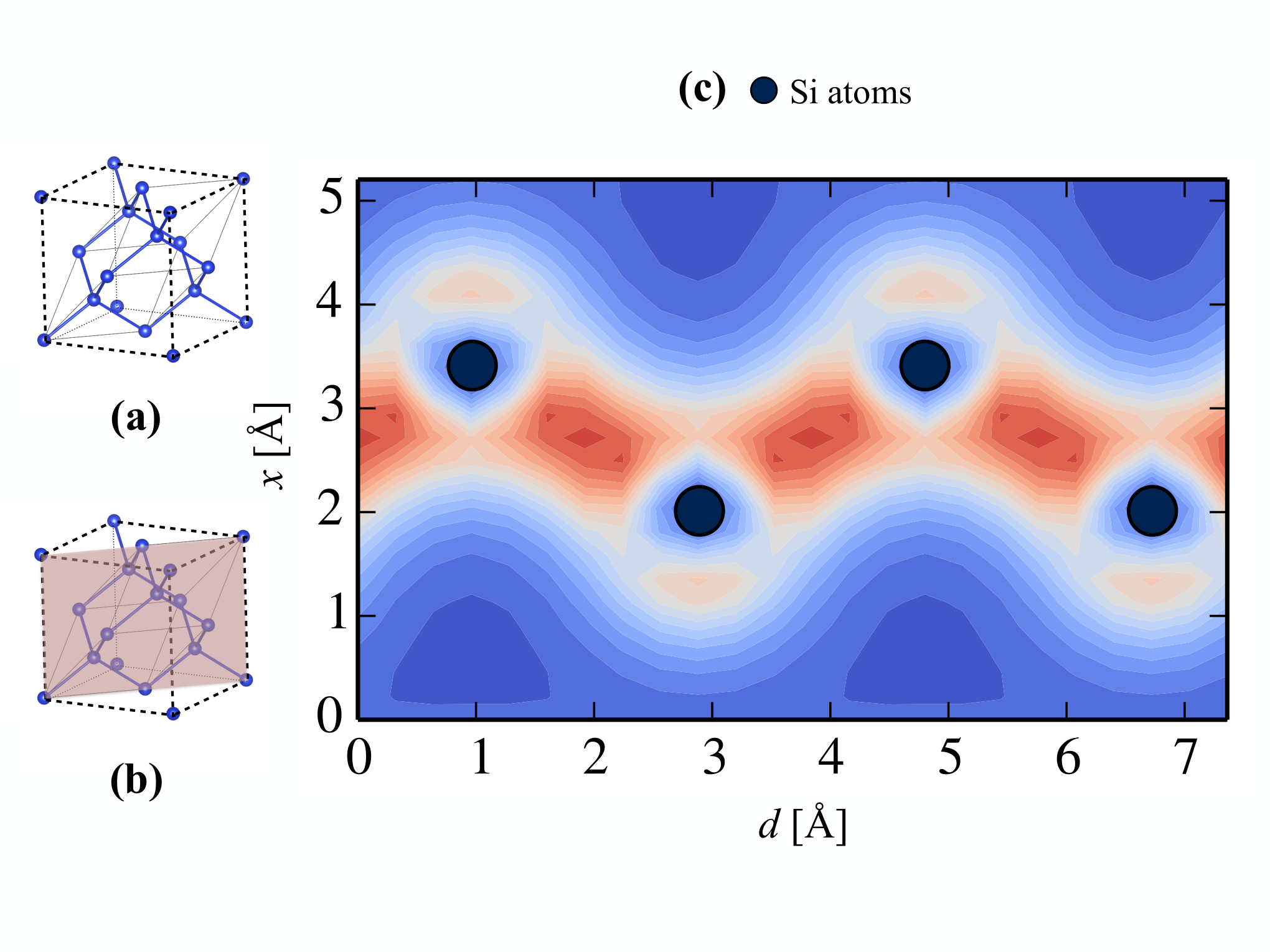
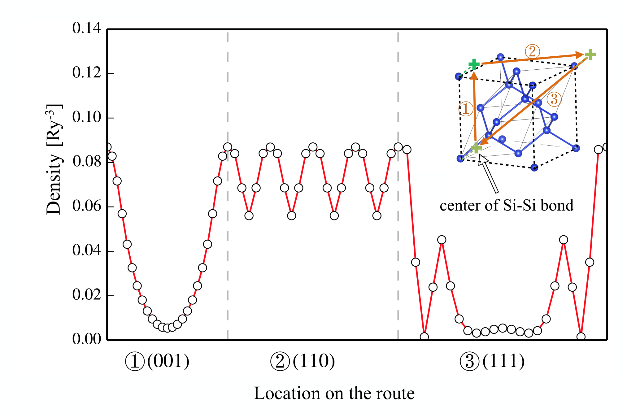
In Si, we plot the density in the plane in Fig. 3. The signature of the Si-Si covalent bond is evident, as a concentration of valence electrons is seen on a line connecting the nearest neighbor Si atoms. Note that there are small bumps located in the vicinity of each Si atom and complementing the two bonds in the plane, which are contributions from two Si-Si bonds pointing out of the plane, reflecting the nature of the hybridization. We also plot the charge density along line cuts in Fig. 4, following the route , which forms a triangle as illustrated in the inset. The origin is taken to be the high-symmetry middle point between two neighboring Si atoms, while and are translated from by lattice constants along the direction connecting them.
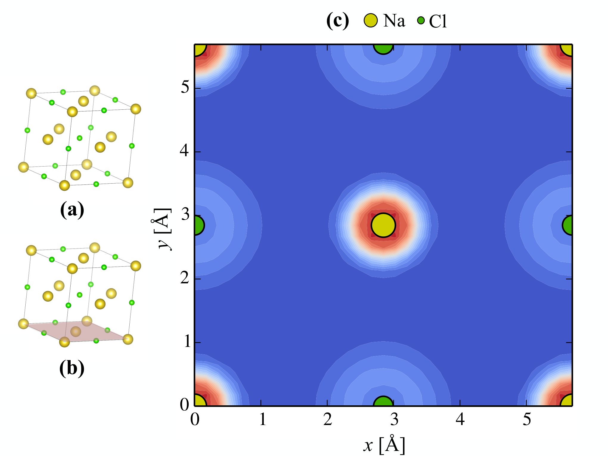
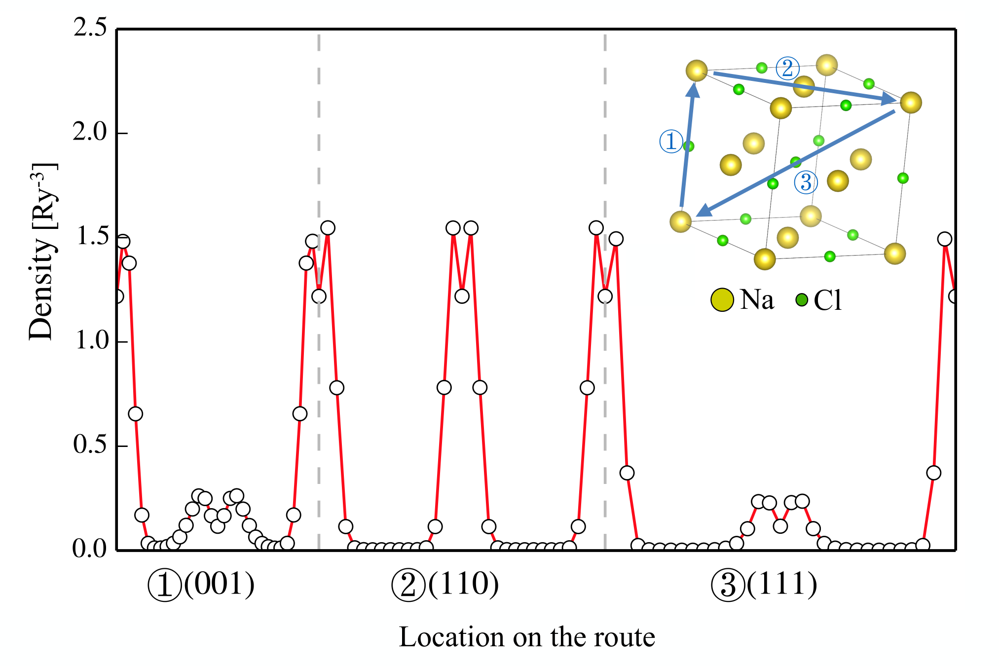
We next present the results for NaCl in a similar fashion. In Fig. 5, the density is shown on the -plane (). Then in Fig. 6, we plot the density along the triangular path, following the route , with the origin taken to be a Na atom. Figure 7 shows the density from a different perspective, illustrating the ionic nature of NaCl. Within a sphere of radius 1 Å centered at a Na atom, the integrated charge density is electron, consistent with a Na+ (with our He-core pseudopotential). This integrated charge density remains saturated with increasing radius, until the sphere reaches the vicinity of the nearest Cl atom. Around a Cl atom, this integrated density also approaches electron when the radius of the sphere is around 2 Å, consistent with a Cl- ion (Ne-core pseudopotential).
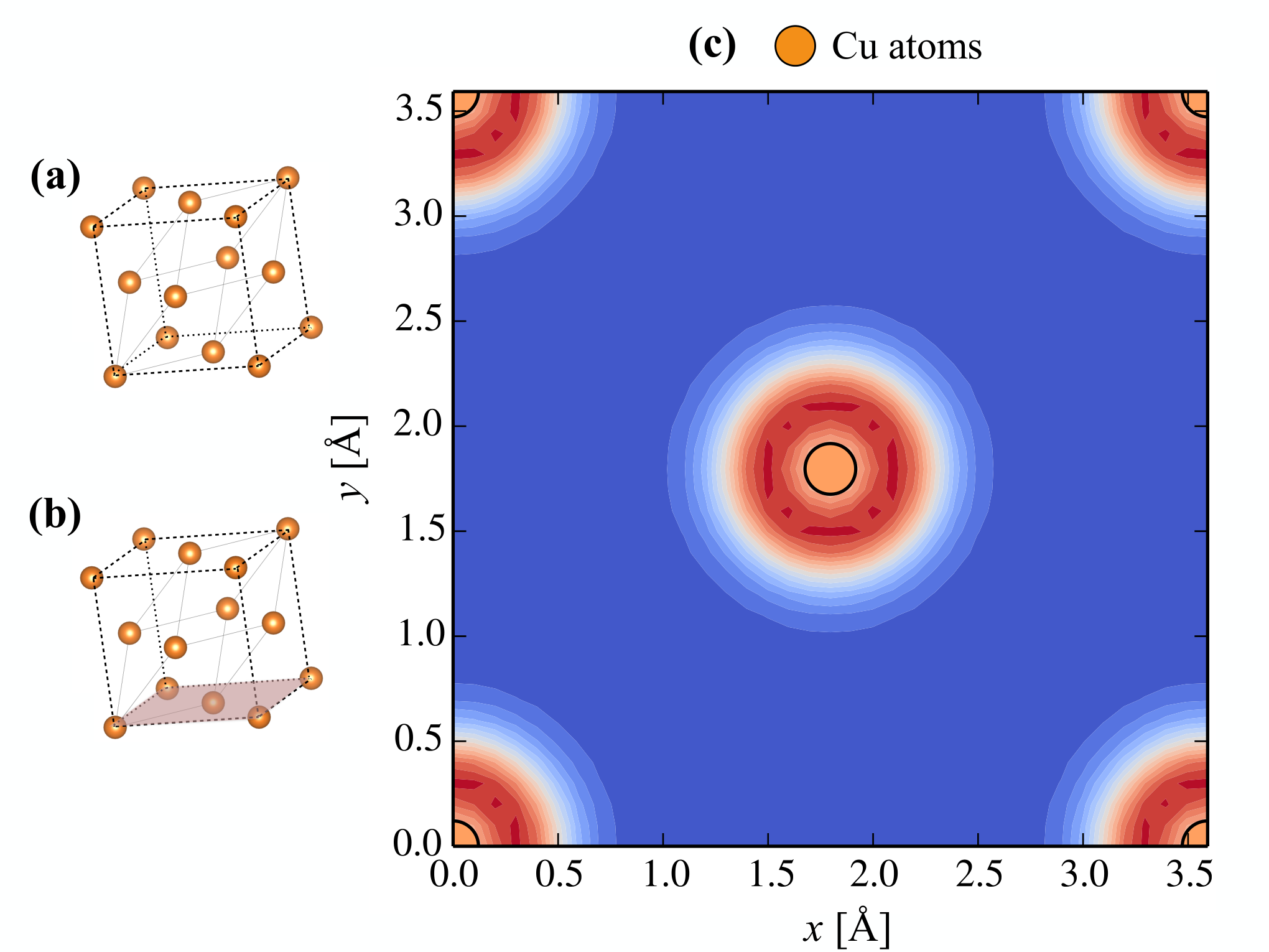
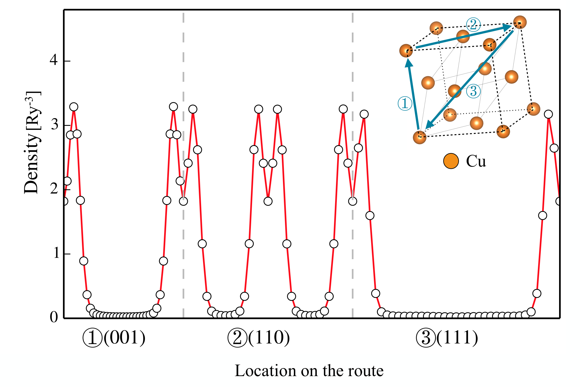
Results for Cu are shown in Figs. 8 and 9. The charge density in Cu bears a resemblance to that of NaCl. However the density scales are very different in Fig. 9, which obscures the significant density in between Cu atoms. The distinction between this metallic system and the ionic crystal NaCl, and the semiconductor Si can be seen more clearly in Fig. 10, in which we plot the distribution of electron densities in each solid. The distribution is characterized by the percentage of the real-space FFT grid points having a given charge density value. (It should be noted that this is in presence of the pseudopotential and without accounting for the core electrons.) We see that a pronounced peak is present in Cu at around , with 55% of FFT grid points in Cu share a density value of , corresponding to an electron Wigner-Seitz radius of Bohr. This is consistent with the notion of a metallic system being characterized as a “uniform electron gas”, and is not seen in NaCl or Si. In particular, NaCl shows a significant concentration in a low-density region, while Si features a broader peak.
V Benchmark DFT functionals
V.1 Comparison of the electronic densities from several functionals with AFQMC results
Based on a variety of benchmark studies (see, for example, Refs. LeBlanc et al. 2015; Williams et al. 2020; Motta et al. 2017), the AFQMC results are expected to be highly accurate. The density results we have presented from AFQMC can serve as a reference in these systems. We next carry out a comparative study of the computed densities from several popular DFT functionals, including: (i) LDA, the local-density approximation by Perdew-Zunger (PZ) (Perdew and Zunger 1981); (ii) PBE, a generalized-gradient approximation (GGA) functional by Perdew-Burke-Ernzerhof (Perdew et al. 1996a); (iii) PBEsol, a revised GGA functional for solids (Perdew et al. 2008); (iv) PBE0, a hybrid functional between PBE and Hartree-Fock (Perdew et al. 1996b); (v) B3LYP, a widely used hybrid functional in quantum chemistry (Stephens et al. 1994). In each DFT calculation, we use the same pseudopotential as in the PW-AFQMC calculations, namely the multiple-projector ONCVPSP generated with LDA. In other words, we adopt the philosophy of viewing the pseudopotential as defining an effective Hamiltonian, and ask how each functional treats this effective Hamiltonian as compared to AFQMC.
In Figs. 11, 12, and 13, we present the result for Si, NaCl, and Cu, respectively, by plotting the densities from the five different DFT functionals against the reference AFQMC density. Density differences and percentage discrepancies are shown in two different panels, following the same line cuts as used in Figs. 4, 6, and 9, respectively. The AFQMC statistical error bars are given by the shades. Additional details on the benchmark are provided in Appendix B.
For Si, PBE and PBE0 perform very well, with average percentage errors of around 2%. B3LYP shows a comparable performance along the route, but is less accurate for the entire cell. LDA and PBEsol show larger errors in general. We see correlations in the location and amount of the errors between all functionals, except for B3LYP whose behavior is more different from the other functionals. In NaCl, the most significant errors occur between Na and Cl atoms, along the diagonal direction. Except for B3LYP, all functionals tend to give a density that is consistently too high in these regions, well outside the AFQMC statistical error. The errors from the five functionals all show some correlation, with B3LYP giving the smallest errors in these regions, followed by PBE and PBE0. In Cu, the behavior of the errors is more subtle. The absolute and relative errors in the plot tell somewhat different stories. B3LYP yields the smallest integrated absolute error along the chosen path, but gives the largest percentage error, and also the second largest integrated absolute error over the entire cell.
V.2 Accuracy of a functional: density vs. total energy
| XC | Input Density | NaCl | Silicon | ||
|---|---|---|---|---|---|
| (Å) | (GPa) | (Å) | (GPa) | ||
| Exp. | 5.640(Barrett and Wallace 1954) | 24.42(Combes et al. 1951) | 5.431(Kittel et al. 1996) | 98.8(Kittel et al. 1996) | |
| LDA | (same) | 5.46 | 32.21 | 5.395 | 95.19 |
| B3LYP | 5.58 | 27.98 | 5.382 | 96.40 | |
| PBEsol | 5.60 | 26.06 | 5.394 | 94.89 | |
| PBE | 5.672 | 24.28 | 5.406 | 92.04 | |
| PBE | B3LYP | 5.681 | 23.27 | 5.408 | 90.65 |
| LDA | 5.682 | 22.93 | 5.404 | 91.53 | |
Although charge density plays a vital role in DFT, the accuracy of the density from a particular exchange-correlation functional does not seem to provide an unambiguous measure of the quality of the functional. We illustrate this point below following the benchmark results on Si and NaCl in the previous subsection.
We perform equation of state (EOS) calculations in these solids to obtain the equilibrium lattice constant and bulk modulus by fitting the total energies using the Murnaghan equation (Murnaghan 1944). The results are tabulated in Table 1, together with the experimental values. In NaCl, PBE yields the best results for both the equilibrium lattice constant and the bulk modulus. However, we recall that B3LYP is the one that yielded the best density. In Si, B3LYP shows the largest error in the lattice constant and the best accuracy in bulk modulus, while PBE is at the opposite, with the smallest error in lattice constant and the largest in bulk modulus, although the margins are all rather small here. On the other hand, the result from the overall electronic density shows no ambiguity and indicates that PBE performs the best, as discussed in Sec. V.1.
To reconcile these inconsistent behaviors in density versus total energy, we examine the effect of the exchange-correlation energy separately from the density. We use the PBE functional to perform a one-shot total energy calculation by feeding it a wave function from B3LYP (or LDA). The wave function is obtained from a converged self-consistent B3LYP calculation, by taking the occupied orbitals. Thus the wavefunction produces the electronic density from the fully self-consistent B3LYP calculation. The resulting EOS using total energies computed from this procedure is re-analyzed, and shown in the bottom two rows, for B3LYP and LDA wave functions respectively. We see that the results in general exhibit only minor variations from the PBE results. In the case of LDA, the improvement is dramatic in NaCl, and mixed in Si, with the bulk modulus becoming worse as it moves towards the PBE result (which also occurs with B3LYP density). This shows that the accuracy of the electronic density is secondary in the performance of an XC functional for computing the EOS, and the primary factor affecting overall performance in these solids is the exchange-correlation energy.
VI Conclusion
We have introduced into the plane-wave AFQMC framework the calculation of observables using a path-restoration back-propagation technique, which is applied to compute the charge density in three typical solids with different crystal bonding mechanisms, the covalent-bond crystal Si, the ionic-bond NaCl, and the transition metal fcc-Cu. The results provide highly accurate ab initio many-body electronic densities in these systems. We compared these results against several of the most popular density functionals. In general, the densities produced by these functionals agree quite well with the PW-AFQMC results. The discrepancies from the different functionals are quantified, and our results can be used for future benchmarks of other computational methods. Additionally, the PW-AFQMC electronic densities may help with the development of improved density functionals.
Besides charge density, the back-propagation technique extends easily to other quantities, including interatomic forces, which can be used to perform accurate molecular dynamics and geometry optimization, as well as to calculate phonon properties and access thermodynamic properties of solids. Work is on-going along these lines.
Acknowledgements.
We thank D. Ceperley, M. Holzmann, H. Krakauer, E. J. Walter and J. Lee for useful discussions. We are grateful to L. Reining for discussions and for pointing out an error in an early version of the manuscript. S.C. would like to thank the Center for Computational Quantum Physics, Flatiron Institute for support and hospitality. We also acknowledge support from the U.S. Department of Energy (DOE) under Grant No. DE-SC0001303. F.M. is supported by the National Natural Science Foundation of China under Grant No. 11674027. The authors thank William & Mary Research Computing and Flatiron Institute Scientific Computing Center for computational resources and technical support. The Flatiron Institute is a division of the Simons Foundation.Appendix A More information on the pseudopotential
Our pseudopotentials for Si, NaCl, and Cu are constructed with Hamann’s multiple-projector optimized norm-conserving pseudopotential (oncvpsp) code (Hamann 2013), using LDA as the exchange correlation functional. The local reference in oncvpsp is a smooth continuation of the all-electron potential from the minimum radius cutoff to 0, using a smooth polynomial ( in oncvpsp input). For compatibility with AFQMC, the nonlinear core correction is turned off in pseudopotential generations.
For Si, the kinetic energy cutoff is 25 Ry and the electron configuration is . The first three orbitals are taken as core orbitals. We use three projectors , all with the same core radius of 2.04 Bohr.
For NaCl, the kinetic energy cutoff is 40 Ry. In Na, the electron configuration is , with only orbital as core, due to the fact that the semi-core electrons of Na have large overlaps with the electron, and neglecting them from the valence was seen to cause errors in the equation of state in AFQMC calculations (Ma et al. 2017). Core radii for the three projectors are 1.82, 2.27, 2.27 Bohr, respectively. In Cl, the electron configuration is , and the first three orbitals are taken as core. The core radii for the three projectors () are 2.72, 2.72, and 3.01 Bohr, respectively.
For Cu, we have used two different pseudopotentials, with Ne-core and Ar-core, both using a kinetic energy cutoff of 64 Ry. The Ne-core pseudopotential, which is the primary one used in the paper, has an electron configuration of . Core radii are 1.60, 1.97, and 1.97 Bohr for the three projectors; the corresponding wave-vector cutoffs are 7.0, 7.75 and 8.0 Ry. For the Ar-core pseudopotential, the electron configuration is , with the first five orbitals being the core orbitals. Core radii for are 2.30, 2.30, and 2.10 Bohr, respectively. The wave-vector cutoff (8 Ry) is the same for all projectors.
Appendix B Supplementary Data on Exchange-Correlation Functional Benchmarks
In Tables 2, 3, and 4, we list the mean absolute error (MAE) in the density of multiple DFT exchange correlation functionals with respect to the near-exact AFQMC density, on the high-symmetry triangular route and the full three-dimensional (3D) real-space grid, for Si, NaCl, and Cu, respectively. The formula for this MAE is
where is the set of real-space grid points, located on the triangular route or the full 3D real-space grid; is the number of grid points in ; and for a given exchange-correlation functional “XC.” For mean percentage difference a similar formula is used,
| MAE ( ) | Mean percentage error (%) | |||
|---|---|---|---|---|
| Triangular route | Full 3D grid | Triangular route | Full 3D grid | |
| AFQMC11 1 AFQMC statistical error | 1.04 | 0.76 | 0.29 | 0.30 |
| LDA | 10.4 | 4.35 | 3.10 | 2.03 |
| PBE | 6.9 | 2.87 | 1.86 | 0.97 |
| PBEsol | 10.6 | 4.21 | 3.12 | 1.77 |
| B3LYP | 7.1 | 3.86 | 2.76 | 2.17 |
| PBE0 | 7.8 | 2.97 | 2.32 | 1.23 |
| MAE ( ) | Mean percentage error (%) | |||
|---|---|---|---|---|
| Triangular route | Full 3D grid | Triangular route | Full 3D grid | |
| AFQMC11 1 AFQMC statistical error | 1.74 | 0.75 | 0.26 | 0.37 |
| LDA | 29.0 | 6.64 | 4.47 | 5.13 |
| PBE | 13.7 | 1.43 | 0.86 | 0.81 |
| PBEsol | 19.0 | 3.11 | 2.40 | 2.49 |
| B3LYP | 12.9 | 1.27 | 0.67 | 0.61 |
| PBE0 | 11.7 | 2.10 | 1.62 | 1.30 |
| MAE ( ) | Mean percentage error (%) | |||
|---|---|---|---|---|
| Triangular route | Full 3D grid | Triangular route | Full 3D grid | |
| AFQMC11 1 AFQMC statistical error | 9.5 | 4.3 | 0.36 | 0.46 |
| LDA | 91.2 | 16.1 | 1.20 | 1.52 |
| PBE | 60.8 | 12.9 | 1.24 | 1.14 |
| PBEsol | 73.7 | 12.3 | 1.43 | 1.39 |
| B3LYP | 44.0 | 21.7 | 2.57 | 2.81 |
| PBE0 | 53.7 | 22.1 | 1.40 | 2.05 |
References
- Hohenberg and Kohn (1964) P. Hohenberg and W. Kohn, Phys. Rev. 136, B864 (1964).
- Jones (2015) R. O. Jones, Rev. Mod. Phys. 87, 897 (2015).
- Becke (2014) A. D. Becke, J. Chem. Phys. 140, 18A301 (2014).
- Burke (2012) K. Burke, J. Chem. Phys. 136, 150901 (2012).
- Ceperley and Alder (1980) D. M. Ceperley and B. J. Alder, Phys. Rev. Lett. 45, 566 (1980).
- Stoudenmire et al. (2012) E. M. Stoudenmire, L. O. Wagner, S. R. White, and K. Burke, Phys. Rev. Lett. 109, 056402 (2012).
- Vogiatzis et al. (2017) K. D. Vogiatzis, D. Ma, J. Olsen, L. Gagliardi, and W. A. de Jong, J. Chem. Phys. 147, 184111 (2017).
- Foulkes et al. (2001) W. M. C. Foulkes, L. Mitas, R. J. Needs, and G. Rajagopal, Rev. Mod. Phys. 73, 33 (2001).
- Reynolds et al. (1982) P. J. Reynolds, D. M. Ceperley, B. J. Alder, and W. A. Lester, J. Chem. Phys. 77, 5593 (1982).
- Zhang and Krakauer (2003) S. Zhang and H. Krakauer, Phys. Rev. Lett. 90, 136401 (2003).
- Motta and Zhang (2018) M. Motta and S. Zhang, WIREs Comput. Mol. Sci. 8, e1364 (2018).
- Hubbard (1959) J. Hubbard, Phys. Rev. Lett. 3, 77 (1959).
- Sugiyama and Koonin (1986) G. Sugiyama and S. Koonin, Annals of Physics (N.Y.) 168, 1 (1986).
- Blankenbecler et al. (1981) R. Blankenbecler, D. J. Scalapino, and R. L. Sugar, Phys. Rev. D 24, 2278 (1981).
- Scalapino and Sugar (1981) D. J. Scalapino and R. L. Sugar, Phys. Rev. B 24, 4295 (1981).
- Zhang et al. (1997) S. Zhang, J. Carlson, and J. E. Gubernatis, Phys. Rev. B 55, 7464 (1997).
- Zhang (2018) S. Zhang, in Handbook of Materials Modeling, edited by W. Andreoni and S. Yip (Springer, Cham, Switzerland, 2018).
- Suewattana et al. (2007) M. Suewattana, W. Purwanto, S. Zhang, H. Krakauer, and E. J. Walter, Phys. Rev. B 75, 245123 (2007).
- Purwanto and Zhang (2004) W. Purwanto and S. Zhang, Phys. Rev. E 70, 056702 (2004).
- Motta and Zhang (2017) M. Motta and S. Zhang, J. Chem. Theor. Comput. 13, 5367 (2017).
- LeBlanc et al. (2015) J. P. F. LeBlanc, A. E. Antipov, F. Becca, I. W. Bulik, G. K.-L. Chan, C.-M. Chung, Y. Deng, M. Ferrero, T. M. Henderson, C. A. Jiménez-Hoyos, E. Kozik, X.-W. Liu, A. J. Millis, N. V. Prokof’ev, M. Qin, G. E. Scuseria, H. Shi, B. V. Svistunov, L. F. Tocchio, I. S. Tupitsyn, S. R. White, S. Zhang, B.-X. Zheng, Z. Zhu, and E. Gull (Simons Collaboration on the Many-Electron Problem), Phys. Rev. X 5, 041041 (2015).
- Zheng et al. (2017) B.-X. Zheng, C.-M. Chung, P. Corboz, G. Ehlers, M.-P. Qin, R. M. Noack, H. Shi, S. R. White, S. Zhang, and G. K.-L. Chan, Science 358, 1155 (2017).
- Motta et al. (2017) M. Motta, D. M. Ceperley, G. K.-L. Chan, J. A. Gomez, E. Gull, S. Guo, C. A. Jiménez-Hoyos, T. N. Lan, J. Li, F. Ma, A. J. Millis, N. V. Prokof’ev, U. Ray, G. E. Scuseria, S. Sorella, E. M. Stoudenmire, Q. Sun, I. S. Tupitsyn, S. R. White, D. Zgid, and S. Zhang (Simons Collaboration on the Many-Electron Problem), Phys. Rev. X 7, 031059 (2017).
- Williams et al. (2020) K. T. Williams, Y. Yao, J. Li, L. Chen, H. Shi, M. Motta, C. Niu, U. Ray, S. Guo, R. J. Anderson, J. Li, L. N. Tran, C.-N. Yeh, B. Mussard, S. Sharma, F. Bruneval, M. van Schilfgaarde, G. H. Booth, G. K.-L. Chan, S. Zhang, E. Gull, D. Zgid, A. Millis, C. J. Umrigar, and L. K. Wagner (Simons Collaboration on the Many-Electron Problem), Phys. Rev. X 10, 011041 (2020).
- Shee et al. (2019) J. Shee, B. Rudshteyn, E. J. Arthur, S. Zhang, D. R. Reichman, and R. A. Friesner, J. Chem. Theor. Comput. 15, 2346 (2019).
- Al-Saidi et al. (2006) W. A. Al-Saidi, S. Zhang, and H. Krakauer, The Journal of Chemical Physics 124, 224101 (2006).
- Ma et al. (2015) F. Ma, W. Purwanto, S. Zhang, and H. Krakauer, Phys. Rev. Lett. 114, 226401 (2015).
- Motta et al. (2020) M. Motta, C. Genovese, F. Ma, Z.-H. Cui, R. Sawaya, G. K.-L. Chan, N. Chepiga, P. Helms, C. Jiménez-Hoyos, A. J. Millis, U. Ray, E. Ronca, H. Shi, S. Sorella, E. M. Stoudenmire, S. R. White, and S. Zhang (Simons Collaboration on the Many-Electron Problem), Phys. Rev. X 10, 031058 (2020).
- Pulay (2014) P. Pulay, Wiley Interdisciplinary Reviews: Computational Molecular Science 4, 169 (2014).
- Purwanto et al. (2009) W. Purwanto, H. Krakauer, and S. Zhang, Phys. Rev. B 80, 214116 (2009).
- Ma et al. (2017) F. Ma, S. Zhang, and H. Krakauer, Phys. Rev. B 95, 165103 (2017).
- Kwee et al. (2008) H. Kwee, S. Zhang, and H. Krakauer, Phys. Rev. Lett. 100, 126404 (2008).
- Born and Oppenheimer (1927) M. Born and R. Oppenheimer, Annalen der physik (Leipzig) 389, 457 (1927).
- Kittel et al. (1996) C. Kittel, P. McEuen, and P. McEuen, Introduction to solid state physics, Vol. 8 (Wiley New York, 1996).
- Martin (2020) R. M. Martin, Electronic Structure: Basic Theory and Practical Methods (Cambridge University Press, Cambridge, England, 2020).
- Ewald (1921) P. P. Ewald, Annalen der physik 369, 253 (1921).
- de Leeuw et al. (1980) S. W. de Leeuw, J. W. Perram, and E. R. Smith, Proceedings of the Royal Society of London. A. Mathematical and Physical Sciences 373, 27 (1980).
- De Leeuw et al. (1980) S. De Leeuw, J. W. Perram, and E. Smith, Proceedings of the Royal Society of London. A. Mathematical and Physical Sciences 373, 57 (1980).
- Thouless (1960) D. J. Thouless, Nuclear Physics 21, 225 (1960).
- Thouless (1961) D. Thouless, Nuclear Physics 22, 78 (1961).
- Shi and Zhang (2021) H. Shi and S. Zhang, The Journal of Chemical Physics 154, 024107 (2021).
- Zhang (2013) S. Zhang, Emergent Phenomena in Correlated Matter: Modeling and Simulation Vol. 3 (Verlag des Forschungszentrum Jülich) (2013).
- Motta (2020) M. Motta, Private Communication (2020).
- Ma et al. (2011) F. Ma, S. Zhang, and H. Krakauer, Phys. Rev. B 84, 155130 (2011).
- Qin et al. (2016) M. Qin, H. Shi, and S. Zhang, Phys. Rev. B 94, 085103 (2016).
- Hamann (2013) D. R. Hamann, Phys. Rev. B 88, 085117 (2013).
- Mohr et al. (2016) P. J. Mohr, D. B. Newell, and B. N. Taylor, Rev. Mod. Phys. 88, 035009 (2016).
- Baldereschi (1973) A. Baldereschi, Phys. Rev. B 7, 5212 (1973).
- Jain et al. (2013) A. Jain, S. P. Ong, G. Hautier, W. Chen, W. D. Richards, S. Dacek, S. Cholia, D. Gunter, D. Skinner, G. Ceder, and K. A. Persson, APL Materials 1, 011002 (2013).
- NaC (2021) “mp-22862: NaCl (cubic, Fm-3m, 225),” Material’s Project (2021), accessed: 2021-01-28.
- Schimka et al. (2011) L. Schimka, J. Harl, and G. Kresse, The Journal of Chemical Physics 134, 024116 (2011).
- Sobol (1967) I. M. Sobol, U.S.S.R. Comput. Maths. Math. Phys. 7, 86 (1967).
- Chen (2020) S. Chen, “github.com/schen24wm/chgden,” (2020).
- Perdew and Zunger (1981) J. P. Perdew and A. Zunger, Phys. Rev. B 23, 5048 (1981).
- Perdew et al. (1996a) J. P. Perdew, K. Burke, and M. Ernzerhof, Phys. Rev. Lett. 77, 3865 (1996a).
- Perdew et al. (2008) J. P. Perdew, A. Ruzsinszky, G. I. Csonka, O. A. Vydrov, G. E. Scuseria, L. A. Constantin, X. Zhou, and K. Burke, Phys. Rev. Lett. 100, 136406 (2008).
- Perdew et al. (1996b) J. P. Perdew, M. Ernzerhof, and K. Burke, The Journal of Chemical Physics 105, 9982 (1996b).
- Stephens et al. (1994) P. J. Stephens, F. J. Devlin, C. F. Chabalowski, and M. J. Frisch, The Journal of Physical Chemistry 98, 11623 (1994).
- Barrett and Wallace (1954) W. T. Barrett and W. E. Wallace, J. Am. Chem. Soc. 76, 366 (1954).
- Combes et al. (1951) L. S. Combes, S. S. Ballard, and K. A. McCarthy, J. Opt. Soc. Am. 41, 215 (1951).
- Murnaghan (1944) F. D. Murnaghan, Proceedings of the National Academy of Sciences 30, 244 (1944).