跳到论文正文
W Papers独立论文阅读器 arXiv:2011.08321 论文正文 计算阅读时间 · 0%
引用这篇论文根据当前论文元数据生成,正式投稿前建议核对。


License: arXiv.org perpetual non-exclusive license
arXiv:2011.08321v2 [math.ST] 26 Aug 2021

Nonparametric Bayesian volatility estimation for gamma-driven stochastic differential equations

Denis Belomestnylabel=e1]denis.belomestny@uni-due.de Email: [    Shota Gugushvililabel=e2]shota@yesdatasolutions.com Email: [    Moritz Schauerlabel=e3]smoritz@chalmers.se Email: [    Peter Spreijlabel=e4]spreij@uva.nl Email: [ Address: Department, Faculty of Mathematics
Duisburg-Essen University
Thea-Leymann-Str. 9
D-45127 Essen
Germany
and Faculty of Computer Sciences
HSE University
Moscow, Russian Federation
Address: Biometris
Wageningen University & Research
Postbus 16
6700 AA Wageningen
The Netherlands
Address: Department of Mathematical Sciences
Chalmers University of Technology and University of Gothenburg
SE-412 96 Göteborg
Sweden
Address: Korteweg-de Vries Institute for Mathematics
Universiteit van Amsterdam
P.O. Box 94248
1090 GE Amsterdam
The Netherlands
and Institute for Mathematics, Astrophysics and Particle Physics
Radboud University
Nijmegen
Netherlands
Abstract

We study a nonparametric Bayesian approach to estimation of the volatility function of a stochastic differential equation driven by a gamma process. The volatility function is modelled a priori as piecewise constant, and we specify a gamma prior on its values. This leads to a straightforward procedure for posterior inference via an MCMC procedure. We give theoretical performance guarantees (minimax optimal contraction rates for the posterior) for the Bayesian estimate in terms of the regularity of the unknown volatility function. We illustrate the method on synthetic and real data examples.

Keywords: 
Stochastic differential equation,
keywords
††email: e1††email: e2††email: e3††email: e4

, and and

1 Introduction

1.1 Problem formulation

The goal of the present paper is Bayesian nonparametric estimation of the positive local scale function σ\sigma that appears in the Lévy-driven stochastic differential equation

d​Xt=σ⁡(Xt−)​d​Lt,X0=0,\mathrm{d}X_{t}=\sigma(X_{t-})\,\mathrm{d}L_{t},\,X_{0}=0, (1)

from observations of the solution XX. Here LL is a gamma process with L0=0L_{0}=0 and therefore LL is a subordinator, i.e. a stochastic process with monotonous sample paths. Furthermore, LL has a Lévy measure ν\nu admitting the Lévy density

v⁡(x)=α​x−1​exp⁡(−β​x),x>0,v(x)=\alpha x^{-1}\exp(-\beta x),\,x>0, (2)

where α\alpha and β\beta are two positive constants. The process LL has independent increments, and Lt−LsL_{t}-L_{s} has a Gamma(α⁡(t−s),β)(\alpha(t-s),\beta) distribution for t>st>s with shape parameter α\alpha and scale parameter 1/β1/\beta, as defined in Section 1.6.

Under the assumption that the function σ\sigma (in view of financial applications we refer to it as volatility function) is measurable and satisfies a linear growth condition, it has been shown in Belomestny et al. 2021 that Equation (1) admits a weak solution that is unique in law. Under the stronger condition that σ\sigma is Lipschitz continuous, Equation (1) even has a unique strong solution, see (Protter 2004, Theorem V.6). Note that XX is a Markov process.

Example 1.

To get an impression of how observations of XX look like, we take XX to solve the Lévy SDE (1) with the volatility function

σ0​(x)=1500​(32+sin⁡(2​π​x)).\sigma_{0}(x)=\frac{1}{500}\left(\frac{3}{2}+\sin(2\pi x)\right). (3)

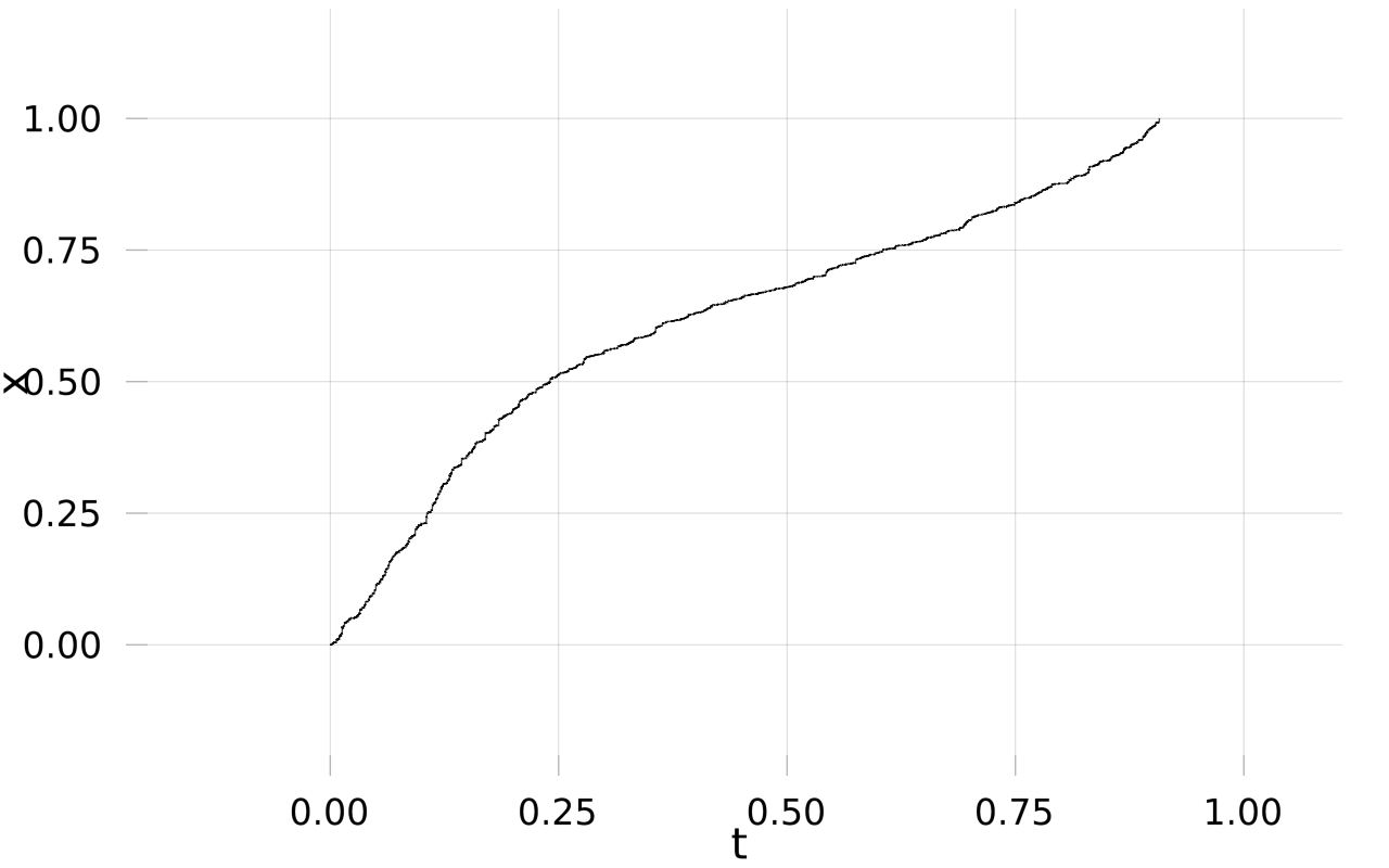
For the driving gamma process LL we take parameters α=1\alpha=1, β=1\beta=1. We used the Euler scheme to generate a single trajectory to serve as observation. We simulated a path traversing the unit interval on a time grid with time step-size δ​t=0.0001\delta t=0.0001 starting in X0=0=b0X_{0}=0=b_{0}. In Section 2.2 we will introduce bins with boundaries bkb_{k} and their hitting times τk\tau_{k}. Approximate hitting times were obtained setting τk′=inf{i​δ​t:Xi​δ​t≥bk}\tau^{\prime}_{k}=\inf\{i\delta t\colon X_{i\delta t}\geq b_{k}\}. Figure 1 shows the sample path until the hitting time τK′\tau^{\prime}_{K} of bK=1b_{K}=1.

Refer to caption
Figure 1: Observation XnX^{n}, n=200n=200, generated from (1) with the Euler scheme with volatility σ0\sigma_{0} given in (3). Parameters of the driving gamma process are α=1\alpha=1, β=1\beta=1.

1.2 Motivation

Gamma processes, that form a special class of Lévy processes (see, e.g., Kyprianou 2014), are a fundamental modelling tool in several fields, e.g. reliability (see van Noortwijk 2009) and risk theory (see Dufresne et al. 1991). Since the driving gamma process LL in (1) has non-decreasing sample paths and the volatility function σ\sigma is non-negative, also the process XX has non-decreasing sample paths. Such processes find applications across various fields. A reliability model as in (1) has been thoroughly investigated from a probabilistic point of view in Wenocur 1989, and constitutes a far-reaching generalisation of a basic gamma model. Furthermore, non-decreasing processes are ideally suited to model revenues from an innovation: in Chance et al. 2008, the authors study the question of pricing options on movie box office revenues that are modelled through a gamma-like stochastic process. Another potential application is in modelling the evolution of forest fire sizes over time, as in Reed & McKelvey 2002.

Any practical application of the model (1) would require knowledge of the volatility function σ\sigma, that has to be inferred from observations on the process XX. In this paper, we will approach estimation of σ\sigma nonparametrically. The latter comes in handy when no apparent functional form for the volatility is available, which usually is the case in practice. Such an approach reduces the risk of model misspecification and allows a honest representation of uncertainties in inferential conclusions (see Silverman 1986 and Müller & Mitra 2013). Recent years have witnessed a tremendous growth of interest and rapid advances in nonparametric Bayesian methods (see, e.g., two monographs Ghosal & van der Vaart 2017 and Müller et al. 2015). Coherence, elegance and automatic uncertainty quantification are some of the widely acknowledged attractive features of a Bayesian approach to statistics. Hence our decision to follow a Bayesian method in this paper. However, we also note that with a careful choice of a prior a nonparametric Bayesian method enjoys very favourable frequentist properties; see, e.g., Ghosal & van der Vaart 2017.

On the theoretical side, we are ultimately interested in asymptotic properties of our Bayesian procedure for estimating the volatility function σ\sigma. To that end we need a sufficiently rich set of observations and this can be accomplished by the scaled observation process in (4) below, instead of XX satisfying (1). So we consider the process XnX^{n} given as the solution to

d​Xtn=1n​σ​(Xt−n)​d​Lt,X0n=0.\mathrm{d}X^{n}_{t}=\frac{1}{n}\sigma(X^{n}_{t-})\,\mathrm{d}L_{t},\,X^{n}_{0}=0. (4)

The scaling factor 1n\frac{1}{n} causes for large values of nn a ‘slow growth’ of the process XnX^{n} and ‘long times’ to reach certain levels. We will thus assume that XnX^{n} is observed on a long time interval [0,Tn][0,T^{n}], where Tn→∞T^{n}\to\infty. Later we will specify TnT^{n} and we will see that TnT^{n} grows roughly proportionally with nn. Asymptotic results will be derived for n→∞n\to\infty. The setup above for having a rich set of observations allows for a different, but equivalent description of the model. Let Ytn=Xn​tnY^{n}_{t}=X^{n}_{nt}. Then YnY^{n} satisfies the SDE

Ytn=∫0tσ⁡(Ys−n)​d​Lsn,Y^{n}_{t}=\int_{0}^{t}\sigma(Y^{n}_{s-})\,\mathrm{d}L^{n}_{s}, (5)

where Ltn=Ln​tnL^{n}_{t}=\frac{L_{nt}}{n}. Note that LnL^{n} is again a gamma process with a Lévy density

vn​(x)=n​αx​exp⁡(−n​β​x),v_{n}(x)=\frac{n\alpha}{x}\exp(-n\beta x),

and (for t>s≥0t>s\geq 0) Ltn−LsnL^{n}_{t}-L^{n}_{s} has a Gamma(n​α​(t−s),n​β)(n\alpha(t-s),n\beta) distribution. Here we see a smoother behaviour of LnL^{n} and hence of YnY^{n} for growing nn. In fact, it can be shown that LnL^{n} weakly converges to the function L∞L^{\infty} given by Lt∞=αβ​tL^{\infty}_{t}=\frac{\alpha}{\beta}t, and as a consequence YnY^{n} should then converge to a deterministic limit as well. This behaviour of the process YnY^{n} bears some similarity to the properties of a diffusion process YεY^{\varepsilon} with small diffusion coefficient (WW is a Wiener process),

Ytε=∫0ta⁡(Ysε)​𝑑s+ε​Wt,Y^{\varepsilon}_{t}=\int_{0}^{t}a(Y^{\varepsilon}_{s})\,\mathrm{d}s+\varepsilon W_{t},

which also has a deterministic limit as ε→0\varepsilon\to 0. The similarity becomes more pronounced, if one writes the semimartingale decomposition of YnY^{n},

Ytn=αβ​∫0tσ⁡(Ys−n)​𝑑s+Mtn,Y^{n}_{t}=\frac{\alpha}{\beta}\int_{0}^{t}\sigma(Y^{n}_{s-})\,\mathrm{d}s+M^{n}_{t},

where, under appropriate conditions, the (local) martingale MnM^{n} vanishes for n→∞n\to\infty. This conceptual similarity with drift estimation in a well-known diffusion model and the statistical problem there, estimation of the function aa, should be understood as a mathematical motivation for our study. Although it is possible to present all results that follow in terms of properties of the process YnY^{n}, we opted to give them for XnX^{n}.

1.3 Literature overview

Statistical inference for Lévy driven SDEs is an active research with many contributions. Let us mention recent works by Jasra et al. 2011, Jasra et al. 2019,Uehara 2019, Gushchin et al. 2019 and Eguchi & Uehara 2020. Such models are popular in finance and econometrics, see e.g. Todorov 2011. In this paper we study the problem of Bayesian inference for the volatility coefficient of a Lévy-driven SDE.

Nonparametric Bayesian literature on inference in the model (1) is non-existent, but somewhat related problems have been considered in several papers. Thus, Belomestny et al. 2019 study a nonparametric Bayesian approach to estimation of the Lévy measure for Lévy processes with monotonous sample paths (subordinators), while Gugushvili et al. 2015, Gugushvili et al. 2018 and Gugushvili et al. 2020 investigate the same problem for compound Poisson processes. There exists also a limited amount of work on nonparametric Bayesian volatility estimation in diffusion models, e.g. Batz et al. 2018 and Nickl & Söhl 2017, but a paper that is most related to the present one is Gugushvili et al. 2019. Finally, Koskela et al. 2019 is a theoretical contribution, where frequentist consistency of a Bayesian approach to inference in jump-diffusion models is established.

1.4 Our contribution

Our work is the first contribution to nonparametric Bayesian volatility estimation for Lévy-driven SDEs. The method we propose is easy to understand, and leads to good practical results in synthetic and real data examples. We expect it to open up new research directions in inference for stochastic differential equations driven by jump processes, both from the practical and theoretical point of views. Our approach is based on a piecewise constant approximation with a proper prior on the corresponding parameters. We show the contraction of the posterior for Hölder continuous volatility coefficients and propose a MCMC procedure for sampling.

Example 2.

We continue Example 1 and graphically illustrate our inferential results. In agreement with the notation pertaining to the asymptotic regime detailed in (4) we took XnX^{n} as the solution to the Lévy SDE (1) with the volatility function

σ0​(x)=32+sin⁡(2​π​x)\displaystyle\sigma_{0}(x)=\frac{3}{2}+\sin(2\pi x) (6)

and scaled it with 1/n1/n, n=500n=500. For details of our Bayesian procedure we refer to Section 2.2, in the present example this comes down to the following.

We have partitioned the unit interval into 1010 bins setting bk=k​δ​xb_{k}=k\delta x, δ​x=0.1,\delta x=0.1, k=1,…,10,k=1,\ldots,10, and used the piecewise constant prior of the form σ⁡(x)=∑kξk​𝟏Bk​(x),\sigma(x)=\sum_{k}\xi_{k}\mathbf{1}_{B_{k}}(x), where ξ1,…,ξ10\xi_{1},\ldots,\xi_{10} are i.i.d. random variables with an inverse gamma distribution. The posterior is given in closed form by (10). Figure 2 contrasts the corresponding marginal 90%90\,\%-posterior credible bands for σ\sigma with the true volatility function σ0\sigma_{0} from (6).

Refer to caption
Figure 2: Red: true volatility σ0\sigma_{0} as a function of xx. Shaded: marginal 90%90\,\%-posterior credible band for the piecewise constant posterior σ\sigma. Black: marginal posterior median.

1.5 Structure of the paper

The paper is organised as follows: in Section 2 we describe in detail our Bayesian method for volatility estimation. In Section 3 we present asymptotic properties of the posterior distribution when the volatility function σ\sigma is piecewise constant, whereas in Section 4 we present such properties when the volatility function is Hölder continuous. The contraction rate we obtain in the latter case is shown to be minimax optimal. Real data examples are considered in Section 5. In Section 6 we consider some extensions and variations of our approach, in particular paying attention to the setting of discrete time observations, and propose a Metropolis-Hastings approach for simulating gamma process bridges.

1.6 Notation

We denote the gamma distribution with shape parameter a>0a>0 and rate parameter b>0b>0 (hence scale 1/b1/b) by Gamma⁡(a,b)\operatorname{Gamma}(a,b). Recall that its density is given by

x↦baΓ⁡(a)​xa−1​e−b​x,x>0,x\mapsto\frac{b^{a}}{\Gamma(a)}x^{a-1}e^{-bx},\quad x>0,

where Γ\Gamma is the gamma function. The inverse gamma distribution with shape parameter a>0a>0 and scale parameter b>0b>0 will be denoted by IG⁡(a,b)\operatorname{IG}(a,b). The corresponding density is

x↦baΓ⁡(a)x−a−1e−b/x,x>0,x\mapsto\frac{b^{a}}{\Gamma(a)}x^{-a-1}e^{-b/x},\quad x>0,

and its expectation and variance are ba−1\frac{b}{a-1} and b2(a−1)2​(a−2),\frac{b^{2}}{(a-1)^{2}(a-2)}, respectively. Following a standard Bayesian convention, we will often use lowercase letters to write random variables. Conditioning of xx on yy will be denoted by x|yx\mid y.

2 Bayesian approach

To compute a posterior distribution, a likelihood ratio is needed. In this section we study likelihood ratios and existence of a weak solution to Equation (1).

2.1 Likelihood

Let (Ω,ℱ,𝔽,ℙ)(\Omega,\mathcal{F},\mathbb{F},\mathbb{P}) be a filtered probability space and let (Lt)t≥0(L_{t})_{t\geq 0} be a gamma process adapted to 𝔽\mathbb{F}, whose Lévy measure admits the density vv given by (2). Assume that XX is a (weak) solution to (1), and assume that XX is observed on an interval [0,T][0,T]. We denote by ℙTσ\mathbb{P}^{\sigma}_{T} (a probability measure on ℱTX=σ(Xt,0≤t≤T)\mathcal{F}^{X}_{T}=\sigma(X_{t},0\leq t\leq T)) its law. In agreement with this notation we let ℙT1\mathbb{P}^{1}_{T} be the law of XX when σ≡1\sigma\equiv 1, in which case Xt=Lt,t∈[0,T]X_{t}=L_{t},\,t\in[0,T]. The measure ℙT1\mathbb{P}^{1}_{T} will serve as a reference measure. The choice σ=1\sigma=1 for obtaining a reference measure is natural, but also arbitrary. Many other choices for the function σ\sigma are conceivable, in particular other constant functions. In Belomestny et al. 2021 the following proposition has been proven.

Proposition 3.

Let σ\sigma be a positive locally bounded measurable function on [0,∞)[0,\infty) such that (1) admits a weak solution that is unique in law. Assume moreover that σ\sigma is lower bounded by a strictly positive constant. Let TT be a finite (stopping) time T>0T>0. Then the laws ℙTσ\mathbb{P}^{\sigma}_{T} and ℙT1\mathbb{P}^{1}_{T} are equivalent on ℱTX\mathcal{F}^{X}_{T} and the corresponding Radon-Nikodym derivative ZTZ_{T} has the explicit representation:

ZT=exp⁡(∫0T∫0∞log⁡Y⁡(t,x)​μX​(𝑑x,𝑑t)−∫0T∫0∞(Y⁡(t,x)−1)​v​(x)​𝑑x​𝑑t),Z_{T}=\exp\left(\int_{0}^{T}\int_{0}^{\infty}\log Y(t,x)\,\mu^{X}(\mathrm{d}x,\mathrm{d}t)-\int_{0}^{T}\int_{0}^{\infty}(Y(t,x)-1)v(x)\,\mathrm{d}x\,\mathrm{d}t\right), (7)

where both double integrals are a.s. finite.

Remark 4.

For statistical inference on σ\sigma one needs a realisation of the random quantity ZTZ_{T}, induced by an observed realisation of XX. The realisation of ZTZ_{T} is then simply obtained by evaluation of the integrals along a path of XX. This causes no difficulties as the integrals in ZTZ_{T} are defined pathwise. We will need (in Corollary 5 below) the result for positive piecewise constant functions σ\sigma, and we will see there that for a realisation of ZTZ_{T} one only needs the observed values of the XτknnX^{n}_{\tau^{n}_{k}}. The stopping times τkn\tau^{n}_{k} will be specified later.

2.2 Piecewise constant volatility prior

In our non-parametric Bayesian approach, we will a priori model σ\sigma as a piecewise constant function. Namely,

σ⁡(x)=∑k=1Kξk​𝟏Bk​(x)\displaystyle\sigma(x)=\sum_{k=1}^{K}\xi_{k}\mathbf{1}_{B_{k}}(x) (8)

for bins B1=[0,b1]B_{1}=[0,b_{1}], Bk=(bk−1,bk],k=2,…,K−1,B_{k}=(b_{k-1},b_{k}],k=2,\ldots,K-1, and BK=(bK−1,bK)B_{K}=(b_{K-1},b_{K}), with appropriately chosen increasing sequence of bin endpoints {bk}\{b_{k}\} and the bin number KK. The bins BkB_{k}’s form a partition of the positive halfline [0,∞)[0,\infty). The {ξk}\{\xi_{k}\} are positive numbers (later on positive random variables). Although we use (8) for our model, we emphasize that the ‘true’ σ\sigma does not need to be piecewise constant. As a final remark we note that when σ\sigma is given by (8), (4) still has a unique solution, obtained as concatenation of stopped gamma processes.

Corollary 5.

Suppose that XnX^{n} is given by (4) with σ\sigma given by (8). Let τkn=inf{t≥0:Xtn≥bk}\tau^{n}_{k}=\inf\{t\geq 0:\,X^{n}_{t}\geq b_{k}\}, k=1,…,K,k=1,\ldots,K, and write T=τKnT=\tau^{n}_{K}. Then

d​ℙTσd​ℙT1=exp⁡{β​∑k=1K[1−n​ξk−1]​(Xτknn−Xτk−1nn)−α​∑k=1K(τkn−τk−1n)​log⁡(ξk/n)}.\displaystyle\frac{\mathrm{d}\mathbb{P}^{\sigma}_{T}}{\mathrm{d}\mathbb{P}^{1}_{T}}=\exp\left\{\beta\sum_{k=1}^{K}\left[1-n\xi_{k}^{-1}\right](X^{n}_{\tau^{n}_{k}}-X^{n}_{\tau^{n}_{k-1}})-\alpha\sum_{k=1}^{K}\left(\tau^{n}_{k}-\tau^{n}_{k-1}\right)\log(\xi_{k}/n)\right\}.
Proof.

We have now Y⁡(t,x)=exp⁡(−β​x​(nσ⁡(Xt−n)−1))Y(t,x)=\exp(-\beta x(\frac{n}{\sigma(X^{n}_{t-})}-1)). It follows from Proposition 3 and Remark 4 that

d​ℙTσd​ℙT1\displaystyle\frac{\mathrm{d}\mathbb{P}^{\sigma}_{T}}{\mathrm{d}\mathbb{P}^{1}_{T}} =\displaystyle= exp{∫(0,T]∫(0,∞){xβ[1−nσ⁡(Xs−n)]}μX(ds,dx)\displaystyle\exp\left\{\int_{(0,T]}\int_{(0,\infty)}\left\{x\beta\left[1-\frac{n}{\sigma(X^{n}_{s-})}\right]\right\}\mu^{X}(\mathrm{d}s,\mathrm{d}x)\right.
−∫0T∫(0,∞)(ex​β​[1−nσ⁡(Xs−n)]−1)v(x)dxds}=exp(I1−I2),\displaystyle\left.-\int_{0}^{T}\int_{(0,\infty)}\left(e^{x\beta\left[1-\frac{n}{\sigma(X^{n}_{s-})}\right]}-1\right)v(x)\,\mathrm{d}x\,\mathrm{d}s\right\}=\exp(I_{1}-I_{2}),

where

I1\displaystyle I_{1} =∫(0,T]∫(0,∞){x​β​[1−nσ⁡(Xs−n)]}​μX​(𝑑s,𝑑x)\displaystyle=\int_{(0,T]}\int_{(0,\infty)}\left\{x\beta\left[1-\frac{n}{\sigma(X^{n}_{s-})}\right]\right\}\mu^{X}(\mathrm{d}s,\mathrm{d}x)
=∑k=1K∫(τk−1n,τkn]∫(0,∞){x​β​[1−nσ⁡(Xs−n)]}​μX​(𝑑s,𝑑x)\displaystyle=\sum_{k=1}^{K}\int_{(\tau^{n}_{k-1},\tau^{n}_{k}]}\int_{(0,\infty)}\left\{x\beta\left[1-\frac{n}{\sigma(X^{n}_{s-})}\right]\right\}\mu^{X}(\mathrm{d}s,\mathrm{d}x)
=∑k=1Kβ⁡[1−nξk]​∫(τk−1n,τkn]∫(0,∞)x​μX​(𝑑s,𝑑x)=β​∑k=1K[1−nξk]​(Xτknn−Xτk−1nn),\displaystyle=\sum_{k=1}^{K}\beta\left[1-\frac{n}{\xi_{k}}\right]\int_{(\tau^{n}_{k-1},\tau^{n}_{k}]}\int_{(0,\infty)}x\mu^{X}(\mathrm{d}s,\mathrm{d}x)=\beta\sum_{k=1}^{K}\left[1-\frac{n}{\xi_{k}}\right](X^{n}_{\tau^{n}_{k}}-X^{n}_{\tau^{n}_{k-1}}),

since σ⁡(Xs−n)=ξk\sigma(X^{n}_{s-})=\xi_{k} for s∈(τk−1n,τkn]s\in(\tau^{n}_{k-1},\tau^{n}_{k}] if τk−1n<τkn\tau^{n}_{k-1}<\tau^{n}_{k}. But the above expression is also valid if τk−1n=τkn\tau^{n}_{k-1}=\tau^{n}_{k}, since then Xτknn−Xτk−1nn=0X^{n}_{\tau^{n}_{k}}-X^{n}_{\tau^{n}_{k-1}}=0. Furthermore, by similar reasoning,

I2=∑k=1K(τkn−τk−1n)​∫ℝ+αx​[e−x​β​n​ξk−1−e−β​x]​𝑑x.\displaystyle I_{2}=\sum_{k=1}^{K}\left(\tau^{n}_{k}-\tau^{n}_{k-1}\right)\int_{\mathbb{R}_{+}}\frac{\alpha}{x}\left[e^{-x\beta n\xi_{k}^{-1}}-e^{-\beta x}\right]\,\mathrm{d}x.

We need an intermediate result. For any c>0c>0 one has ∫ℝ+1x[e−xβ/c−e−x​β]dx=∫ℝ+1x[e−x/c−e−x]dx\int_{\mathbb{R}_{+}}\frac{1}{x}\left[e^{-x\beta/c}-e^{-x\beta}\right]\,\mathrm{d}x=\int_{\mathbb{R}_{+}}\frac{1}{x}\left[e^{-x/c}-e^{-x}\right]\,\mathrm{d}x and

∫ℝ+1x[e−x/c−e−x]dx\displaystyle\int_{\mathbb{R}_{+}}\frac{1}{x}\left[e^{-x/c}-e^{-x}\right]\,\mathrm{d}x =∫0∞∫11/c−e−u​xdudx\displaystyle=\int_{0}^{\infty}\int_{1}^{1/c}-e^{-ux}\,\mathrm{d}u\,\mathrm{d}x
=∫11/c∫0∞−e−u​xdxdu\displaystyle=\int_{1}^{1/c}\int_{0}^{\infty}-e^{-ux}\,\mathrm{d}x\,\mathrm{d}u
=∫11/c−1udu=logc.\displaystyle=\int_{1}^{1/c}-\frac{1}{u}\,\mathrm{d}u=\log c.

Application of this result to c=ξk/nc=\xi_{k}/n gives I2=α​∑k(τkn−τk−1n)​log⁡(ξk/n)I_{2}=\alpha\sum_{k}\left(\tau^{n}_{k}-\tau^{n}_{k-1}\right)\log(\xi_{k}/n). ∎

3 Observations with piecewise constant volatility

In this section we will provide contraction rates for the posterior distribution in our Bayesian setup, when the true volatility function σ\sigma is piecewise constant. So, we consider the process XnX^{n} whose true distribution results from XnX^{n} being the solution to

d​Xtn=1n​∑k=1Kσk​𝟏Bk​(Xt−n)​d​Lt,\mathrm{d}X^{n}_{t}=\frac{1}{n}\sum_{k=1}^{K}\sigma_{k}\mathbf{1}_{B_{k}}(X^{n}_{t-})\mathrm{d}L_{t}, (9)

where the constants σk\sigma_{k} are assumed to be strictly positive. So σ⁡(x)=∑kσk​𝟏Bk​(x)\sigma(x)=\sum_{k}\sigma_{k}\mathbf{1}_{B_{k}}(x), in agreement with (4). We assume that the process XnX^{n} is observed until the time where it surpasses the fixed and known level bKb_{K}. We aim at estimating σ\sigma, or equivalently, the sequence {σk}\{\sigma_{k}\}, in a consistent way. In order to accomplish this, the observed process has to spend large times in the bins BkB_{k}, which is effectively the result of the scaling factor 1n\frac{1}{n} for large nn in (9). In fact, one has that the τkn−τk−1n\tau^{n}_{k}-\tau^{n}_{k-1} are roughly proportional to nn for n→∞n\to\infty, see Proposition 8 below for the precise result. In our Bayesian approach we model the σk\sigma_{k} as independent random variables ξk\xi_{k} and we take inverse gamma distributions as a prior for each of them, that is ξk∼IG⁡(αk,βk)\xi_{k}\sim\operatorname{IG}(\alpha_{k},\beta_{k}). Therefore, we have to extend the original probability space to carry the ξk\xi_{k} as well, taking into account that LL and the σk\sigma_{k} have to be independent. We can then use Corollary 5, where ℙTσ\mathbb{P}^{\sigma}_{T} is to be interpreted as the conditional law of XnX^{n} on [0,T][0,T] given the ξk\xi_{k}.

Let x1,…,xKx_{1},\ldots,x_{K} denote realisations of ξ1,…​ξK\xi_{1},\ldots\xi_{K} and let XnX^{n} stand for the path Xtn,X_{t}^{n}, t∈[0,T]t\in[0,T]. With T=τKnT=\tau^{n}_{K}, we then have from Corollary 5 that the posterior joint density of (ξ1,…,ξK)(\xi_{1},\ldots,\xi_{K}) is given by

Π⁡(x1,…,xK∣Xn)∝∏k=1Kexp⁡(−(n​β​(Xτknn−Xτk−1nn)+βk)​xk−1)​xk−α⁡(τkn−τk−1n)−αk−1.\Pi(x_{1},\ldots,x_{K}\mid X^{n})\propto\prod_{k=1}^{K}\exp\left(-(n\beta(X^{n}_{\tau^{n}_{k}}-X^{n}_{\tau^{n}_{k-1}})+\beta_{k})x_{k}^{-1}\right)x_{k}^{-\alpha(\tau^{n}_{k}-\tau^{n}_{k-1})-\alpha_{k}-1}.

It follows that the ξk\xi_{k} are independent under the posterior distribution, and

ξk|Xn∼IG⁡(α​Δ​τkn+αk,n​β​Δ​Xτkn+βk),\xi_{k}\mid X^{n}\sim\operatorname{IG}(\alpha\Delta\tau^{n}_{k}+\alpha_{k},n\beta\Delta X_{\tau^{n}_{k}}+\beta_{k}), (10)

where Δ​τkn=τkn−τk−1n\Delta\tau^{n}_{k}=\tau^{n}_{k}-\tau^{n}_{k-1}, Δ​Xτkn=Xτkn−Xτk−1n\Delta X_{\tau^{n}_{k}}=X_{\tau^{n}_{k}}-X_{\tau^{n}_{k-1}}.

3.1 Result on the overshoot

To prepare for our first main result, we need a property of the overshoots of XnX^{n}. The overshoot POTkn\mathrm{POT}^{n}_{k} is defined as POTkn:=Xτknn−bk≥0\mathrm{POT}^{n}_{k}:=X^{n}_{\tau^{n}_{k}}-b_{k}\geq 0 for k=0,…,Kk=0,\ldots,K. Note that POT0n=0\mathrm{POT}^{n}_{0}=0.

Lemma 6.

Let σK∗=max⁡{σ1,…,σK}\sigma^{*}_{K}=\max\{\sigma_{1},\ldots,\sigma_{K}\} and δ>0\delta>0. The probability ℙ⁡(POTkn<δ)\mathbb{P}(\mathrm{POT}^{n}_{k}<\delta) satisfies the following bound,

ℙ(POTkn<δ)≥bKbK+δ(1−exp(−nδβ/σK∗)).\mathbb{P}(\mathrm{POT}^{n}_{k}<\delta)\geq\frac{b_{K}}{b_{K}+\delta}(1-\exp(-n\delta\beta/\sigma^{*}_{K})). (11)

If δn→0\delta_{n}\to 0 such that n​δn→∞n\delta_{n}\to\infty, then ℙ⁡(POTkn>δn)→0\mathbb{P}(\mathrm{POT}^{n}_{k}>\delta_{n})\to 0.

Proof.

Since POT0n=0\mathrm{POT}^{n}_{0}=0, inequality (11) is trivially true for k=0k=0, so we let k∈{1,…,K}k\in\{1,\ldots,K\} and 0<a<bk0<a<b_{k}. We start by considering the conditional probability ℙ⁡(POTkn<δ∣Xτkn−n=bk−a)\mathbb{P}(\mathrm{POT}^{n}_{k}<\delta\mid X^{n}_{\tau^{n}_{k}-}=b_{k}-a) and we claim that

ℙ⁡(POTkn<δ∣Xτkn−n=bk−a)=νnk([a,a+δ))νkn​([a,∞)),\mathbb{P}(\mathrm{POT}^{n}_{k}<\delta\mid X^{n}_{\tau^{n}_{k}-}=b_{k}-a)=\frac{\nu^{n}_{k}([a,a+\delta))}{\nu^{n}_{k}([a,\infty))}, (12)

where νkn\nu^{n}_{k} is the Lévy measure of the process σkn​L\frac{\sigma_{k}}{n}L. Note that νkn​([a,b])=ν⁡([a​n/σk,b​n/σk])\nu^{n}_{k}([a,b])=\nu([an/\sigma_{k},bn/\sigma_{k}]) with ν\nu the Lévy measure of LL. To see (12), we argue as follows. First we have

ℙ⁡(POTkn<δ∣Xτkn−n=bk−a)\displaystyle\mathbb{P}(\mathrm{POT}^{n}_{k}<\delta\mid X^{n}_{\tau^{n}_{k}-}=b_{k}-a) =ℙ⁡(Δ​Xτknn<bk−Xτk−nn+δ∣Xτkn−n=bk−a)\displaystyle=\mathbb{P}(\Delta X^{n}_{\tau^{n}_{k}}<b_{k}-X^{n}_{\tau^{n}_{k-}}+\delta\mid X^{n}_{\tau^{n}_{k}-}=b_{k}-a)
=ℙ⁡(Δ​Xτknn<a+δ∣Xτkn−n=bk−a).\displaystyle=\mathbb{P}(\Delta X^{n}_{\tau^{n}_{k}}<a+\delta\mid X^{n}_{\tau^{n}_{k}-}=b_{k}-a).

We will now use (Kyprianou 2014, Theorem 5.6), that states in terms of densities (which exist here) and in notation adapted to our situation that the random vector (Xτknn−bk,bk−Xτkn−n)(X^{n}_{\tau^{n}_{k}}-b_{k},b_{k}-X^{n}_{\tau^{n}_{k}-}) has joint density (for x>0x>0, 0<y<bk0<y<b_{k})

fXτknn−bk,bk−Xτkn−n​(x,y)=fU​(bk−y)​fν​(x+y),f_{X^{n}_{\tau^{n}_{k}}-b_{k},b_{k}-X^{n}_{\tau^{n}_{k}-}}(x,y)=f_{U}(b_{k}-y)f_{\nu}(x+y),

where fUf_{U} is the density of the potential function UU (in Kyprianou’s terminology; it will turn out that the precise form of fUf_{U} is not relevant in our context) and fνf_{\nu} the density of the Lévy measure of the process, in our case νkn\nu^{n}_{k}, as we effectively deal with properties of the process σkn​L\frac{\sigma_{k}}{n}L. It follows that bk−Xτkn−nb_{k}-X^{n}_{\tau^{n}_{k}-} has marginal density

fbk−Xτkn−n​(y)=fU​(bk−y)​νkn​([y,∞)).f_{b_{k}-X^{n}_{\tau^{n}_{k}-}}(y)=f_{U}(b_{k}-y)\nu^{n}_{k}([y,\infty)).

Using the change of variables (Xτknn−bk,bk−Xτkn−n)→(Δ​Xτknn,bk−Xτkn−n)(X^{n}_{\tau^{n}_{k}}-b_{k},b_{k}-X^{n}_{\tau^{n}_{k}-})\to(\Delta X^{n}_{\tau^{n}_{k}},b_{k}-X^{n}_{\tau^{n}_{k}-}) one gets from the transformation formula that (Δ​Xτknn,bk−Xτkn−n)(\Delta X^{n}_{\tau^{n}_{k}},b_{k}-X^{n}_{\tau^{n}_{k}-}) has density

fΔ​Xτknn,bk−Xτkn−n​(x,y)=fXτknn−bk,bk−Xτkn−n​(x−y,y)=fU​(bk−y)​fνkn​(x),f_{\Delta X^{n}_{\tau^{n}_{k}},b_{k}-X^{n}_{\tau^{n}_{k}-}}(x,y)=f_{X^{n}_{\tau^{n}_{k}}-b_{k},b_{k}-X^{n}_{\tau^{n}_{k}-}}(x-y,y)=f_{U}(b_{k}-y)f_{\nu^{n}_{k}}(x),

for x>yx>y, 0<y<bk0<y<b_{k} and zero elsewhere. It follows that the conditional density of Δ​Xτknn\Delta X^{n}_{\tau^{n}_{k}} given bk−Xτkn−n=ab_{k}-X^{n}_{\tau^{n}_{k}-}=a is, for x>ax>a,

fΔ​Xτknn|bk−Xτkn−n=a​(x)=fU​(bk−a)​fνkn​(x)fU​(bk−a)​νkn​([a,∞))=fνkn​(x)νkn​([a,∞)).f_{\Delta X^{n}_{\tau^{n}_{k}}\mid b_{k}-X^{n}_{\tau^{n}_{k}-}=a}(x)=\frac{f_{U}(b_{k}-a)f_{\nu^{n}_{k}}(x)}{f_{U}(b_{k}-a){\nu^{n}_{k}}([a,\infty))}=\frac{f_{\nu^{n}_{k}}(x)}{\nu^{n}_{k}([a,\infty))}.

Hence,

ℙ⁡(Δ​Xτknn<a+δ∣Xτkn−n=bk−a)\displaystyle\mathbb{P}(\Delta X^{n}_{\tau^{n}_{k}}<a+\delta\mid X^{n}_{\tau^{n}_{k}-}=b_{k}-a) =∫aa+δfνkn​(x)νkn​([a,∞))​𝑑x\displaystyle=\int_{a}^{a+\delta}\frac{f_{\nu^{n}_{k}}(x)}{{\nu^{n}_{k}}([a,\infty))}\,\mathrm{d}x
=νkn​(a,a+δ)νkn​([a,∞)),\displaystyle=\frac{{\nu^{n}_{k}}(a,a+\delta)}{{\nu^{n}_{k}}([a,\infty))},

which proves (12). Next we show that g⁡(a):=F⁡(a+δ)−F⁡(a)1−F⁡(a)g(a):=\frac{F(a+\delta)-F(a)}{1-F(a)} is decreasing as a function of aa for a≥εa\geq\varepsilon, where ε>0\varepsilon>0 is sufficiently small. Here FF is the ‘truncated distribution function’ of ν\nu, F⁡(x)=ν⁡((ε,x])F(x)=\nu((\varepsilon,x]) for x≥εx\geq\varepsilon. Without loss of generality, we scale FF such that F⁡(∞)=1F(\infty)=1. Then, denoting by ff the derivative of FF, one has

dd​a​F⁡(a+δ)−F⁡(a)1−F⁡(a)\displaystyle\frac{\mathrm{d}}{\mathrm{d}a}\frac{F(a+\delta)-F(a)}{1-F(a)} =(1−F⁡(a))​f​(a+δ)−(1−F⁡(a+δ))​f​(a)(1−F⁡(a))2⏟=:c>0\displaystyle=\frac{(1-F(a))f(a+\delta)-(1-F(a+\delta))f(a)}{\underbrace{(1-F(a))^{2}}_{=:c>0}}
=1c​∫a∞f⁡(x)​f​(a+δ)​𝑑x−1c​∫a+δ∞f⁡(x)​f​(a)​𝑑x\displaystyle=\frac{1}{c}\int_{a}^{\infty}f(x)f(a+\delta)\mathrm{d}x-\frac{1}{c}\int_{a+\delta}^{\infty}f(x)f(a)\mathrm{d}x
=1c​∫a∞(f⁡(x)​f​(a+δ)−f⁡(x+δ)​f​(a))​𝑑x.\displaystyle=\frac{1}{c}\int_{a}^{\infty}\left(f(x)f(a+\delta)-f(x+\delta)f(a)\right)\mathrm{d}x.

With ν⁡(d​x)=f⁡(x)​d​x=αx​exp⁡(−β​x)​d​x\nu(\mathrm{d}x)=f(x)\mathrm{d}x=\frac{\alpha}{x}\exp(-\beta x)\mathrm{d}x for every α\alpha and β\beta (which we later replace with n​βσk\frac{n\beta}{\sigma_{k}}),

dd​a​ℙ​(POTkn<δ∣Xτkn−n=bk−a)\displaystyle\frac{\mathrm{d}}{\mathrm{d}a}\mathbb{P}(\mathrm{POT}^{n}_{k}<\delta\mid X^{n}_{\tau^{n}_{k}-}=b_{k}-a)
=1c​∫a∞(1(a+δ)​x−1(x+δ)​a)​exp⁡(−β⁡(x+δ+a))​𝑑x\displaystyle=\frac{1}{c}\int_{a}^{\infty}\left(\frac{1}{(a+\delta)x}-\frac{1}{(x+\delta)a}\right)\exp(-\beta(x+\delta+a))\mathrm{d}x
=1c​∫a∞(δ⁡(a−x)a​x​(x+δ)​(a+δ))⏟≤0​exp⁡(−β⁡(x+δ+a))​𝑑x≤0.\displaystyle=\frac{1}{c}\int_{a}^{\infty}\underbrace{\left(\frac{\delta(a-x)}{ax(x+\delta)(a+\delta)}\right)}_{\leq 0}\exp(-\beta(x+\delta+a))\mathrm{d}x\leq 0.

Noting that g⁡(a)g(a) is defined for any aa away from zero, we now apply the decreasing behaviour of gg, g⁡(a)≥g⁡(bK)g(a)\geq g(b_{K}) as a<bk<bKa<b_{k}<b_{K}, (with β\beta replaced with n​β/σkn\beta/\sigma_{k}) to get the lower bound

ℙ⁡(POTkn<δ∣Xτkn−n=bk−a)=g⁡(a)≥g⁡(bK)=νnk([bK,bK+δ))νkn​([bK,∞)).\mathbb{P}(\mathrm{POT}^{n}_{k}<\delta\mid X^{n}_{\tau^{n}_{k}-}=b_{k}-a)=g(a)\geq g(b_{K})=\frac{\nu^{n}_{k}([b_{K},b_{K}+\delta))}{\nu^{n}_{k}([b_{K},\infty))}. (13)

Next we will obtain upper and lower bounds for the fraction q⁡(n,a,k,δ)=νnk([a,a+δ))νkn​([a,∞))q(n,a,k,\delta)=\frac{\nu^{n}_{k}([a,a+\delta))}{\nu^{n}_{k}([a,\infty))} for any aa and kk. We write the fraction as a fraction of integrals keeping in mind our model with volatility scaled by nn and LL a gamma process. We will provide bounds on νkn​([a,b))\nu^{n}_{k}([a,b)) with a<b≤∞a<b\leq\infty. We use that for Xt−n∈BkX^{n}_{t-}\in B_{k} we have to deal with the Lévy measure νkn\nu^{n}_{k} with density

vkn(x)=αxexp(−nβx/σk).v^{n}_{k}(x)=\frac{\alpha}{x}\exp(-n\beta x/\sigma_{k}).

We compute

νkn​([a,b))\displaystyle\nu^{n}_{k}([a,b)) =∫abαxexp(−nβx/σk)dx\displaystyle=\int_{a}^{b}\frac{\alpha}{x}\exp(-n\beta x/\sigma_{k})\,\mathrm{d}x
=∫a​n​β/σkb​n​β/σkαy​exp⁡(−y)​𝑑y\displaystyle=\int_{an\beta/\sigma_{k}}^{bn\beta/\sigma_{k}}\frac{\alpha}{y}\exp(-y)\,\mathrm{d}y
≤∫a​n​β/σkb​n​β/σkαa​n​β/σk​exp⁡(−y)​𝑑y\displaystyle\leq\int_{an\beta/\sigma_{k}}^{bn\beta/\sigma_{k}}\frac{\alpha}{an\beta/\sigma_{k}}\exp(-y)\,\mathrm{d}y
=α​σka​n​β(exp(−anβ/σk)−exp(−bnβ/σk)).\displaystyle=\frac{\alpha\sigma_{k}}{an\beta}(\exp(-an\beta/\sigma_{k})-\exp(-bn\beta/\sigma_{k})).

Via a similar argument, we have a lower bound

νkn([a,b))≥α​σkb​n​β(exp(−anβ/σk)−exp(−bnβ/σk)).\nu^{n}_{k}([a,b))\geq\frac{\alpha\sigma_{k}}{bn\beta}(\exp(-an\beta/\sigma_{k})-\exp(-bn\beta/\sigma_{k})).

Hence, using the lower bound with b=a+δb=a+\delta and the upper bound with b=∞b=\infty, we obtain

q(n,a,k,δ)≥aa+δ(1−exp(−nδβ/σk)).q(n,a,k,\delta)\geq\frac{a}{a+\delta}(1-\exp(-n\delta\beta/\sigma_{k})). (14)

Applying (14) to (13), we obtain

ℙ(POTkn<δ∣Xτkn−n=bk−a)≥bKbK+δ(1−exp(−nδβ/σk)).\mathbb{P}(\mathrm{POT}^{n}_{k}<\delta\mid X^{n}_{\tau^{n}_{k}-}=b_{k}-a)\geq\frac{b_{K}}{b_{K}+\delta}(1-\exp(-n\delta\beta/\sigma_{k})).

As the above lower bound is a decreasing function of σk\sigma_{k}, we can make it smaller by replacing σk\sigma_{k} with σK∗\sigma^{*}_{K} and obtain

ℙ(POTkn<δ∣Xτkn−n=bk−a)≥bKbK+δ(1−exp(−nδβ/σK∗)).\mathbb{P}(\mathrm{POT}^{n}_{k}<\delta\mid X^{n}_{\tau^{n}_{k}-}=b_{k}-a)\geq\frac{b_{K}}{b_{K}+\delta}(1-\exp(-n\delta\beta/\sigma^{*}_{K})).

Write μkn\mu^{n}_{k} for the distribution of Xτkn−nX^{n}_{\tau^{n}_{k}-}. Then the unconditional probability ℙ⁡(POTkn<δ)\mathbb{P}(\mathrm{POT}^{n}_{k}<\delta) can be written as

ℙ⁡(POTkn<δ)\displaystyle\mathbb{P}(\mathrm{POT}^{n}_{k}<\delta) =∫[bk−1,bk)ℙ⁡(POTkn<δ∣Xτkn−n=x)​μkn​(𝑑x)\displaystyle=\int_{[b_{k-1},b_{k})}\mathbb{P}(\mathrm{POT}^{n}_{k}<\delta\mid X^{n}_{\tau^{n}_{k}-}=x)\,\mu^{n}_{k}(\mathrm{d}x)
≥∫[bk−1,bk)bKbK+δ(1−exp(−nδβ/σK∗))μkn(dx)\displaystyle\geq\int_{[b_{k-1},b_{k})}\frac{b_{K}}{b_{K}+\delta}(1-\exp(-n\delta\beta/\sigma^{*}_{K}))\,\mu^{n}_{k}(\mathrm{d}x)
=bKbK+δ(1−exp(−nδβ/σK∗)),\displaystyle=\frac{b_{K}}{b_{K}+\delta}(1-\exp(-n\delta\beta/\sigma^{*}_{K})),

which proves (11). The final assertion on ℙ⁡(POTkn<δn)\mathbb{P}(\mathrm{POT}^{n}_{k}<\delta_{n}) for δn→0\delta_{n}\to 0 immediately follows from (11). ∎

3.2 Posterior contraction rate

Statements on convergence in probability refer to the law ℙ=ℙσ,n\mathbb{P}=\mathbb{P}^{\sigma,n} of the process satisfying the SDE (4). We will denote the posterior distribution of the ξk\xi_{k} by Πn\Pi_{n} and posterior expectation and variance by 𝔼Πn\mathbb{E}_{\Pi_{n}} and 𝕍​arΠn{\rm{\mathbb{V}ar}_{\Pi_{n}}}, respectively. Furthermore we write Δ​bk:=bk−bk−1\Delta b_{k}:=b_{k}-b_{k-1} for k≥1k\geq 1.

Lemma 7.

Let δn>0\delta_{n}>0 and Gkn={POTkn>δn}G^{n}_{k}=\{\mathrm{POT}^{n}_{k}>\delta_{n}\} for k≥0k\geq 0. Then it holds for t≥0t\geq 0 and k≥1k\geq 1 that

ℙ⁡(Lt<n⁡(Δ​bk−δn)σk)​ℙ​((Gk−1n)c)≤ℙ⁡(Δ​τkn>t)≤ℙ⁡(Lt<n​Δ​bkσk).\mathbb{P}\Bigl(L_{t}<\frac{n(\Delta b_{k}-\delta_{n})}{\sigma_{k}}\Bigr)\mathbb{P}((G^{n}_{k-1})^{c})\leq\mathbb{P}(\Delta\tau^{n}_{k}>t)\leq\mathbb{P}(L_{t}<\frac{n\Delta b_{k}}{\sigma_{k}}).
Proof.

Let t≥0t\geq 0. On the event {Δτkn>t}\{\Delta\tau^{n}_{k}>t\} we have bk−1≤Xτk−1nn<bkb_{k-1}\leq X^{n}_{\tau^{n}_{k-1}}<b_{k} and for s∈(τk−1n,τkn]s\in(\tau^{n}_{k-1},\tau^{n}_{k}], one has σ⁡(Xs−n)=σk\sigma(X^{n}_{s-})=\sigma_{k}. Hence

ℙ⁡(Δ​τkn>t)\displaystyle\mathbb{P}(\Delta\tau^{n}_{k}>t) =ℙ⁡(Xt+τk−1nn<bk)\displaystyle=\mathbb{P}(X^{n}_{t+\tau^{n}_{k-1}}<b_{k})
=ℙ⁡(Xτk−1nn+1n​∫τk−1nt+τk−1nσ⁡(Xs−n)​d​Ls<bk)\displaystyle=\mathbb{P}\Bigl(X^{n}_{\tau^{n}_{k-1}}+\frac{1}{n}\int_{\tau^{n}_{k-1}}^{t+\tau^{n}_{k-1}}\sigma(X^{n}_{s-})\mathrm{d}L_{s}<b_{k}\Bigr)
=ℙ⁡(σk​(Lt+τk−1n−Lτk−1n)<n⁡(bk−Xτk−1nn))\displaystyle=\mathbb{P}\Bigl(\sigma_{k}(L_{t+\tau^{n}_{k-1}}-L_{\tau^{n}_{k-1}})<n(b_{k}-X^{n}_{\tau^{n}_{k-1}})\Bigr)
=ℙ⁡(Ltn,k<n⁡(Δ​bk−POTk−1n)σk),\displaystyle=\mathbb{P}\Bigl(L^{n,k}_{t}<\frac{n(\Delta b_{k}-\mathrm{POT}^{n}_{k-1})}{\sigma_{k}}\Bigr), (15)

where Ltn,k=Lt+τk−1n−Lτk−1nL^{n,k}_{t}=L_{t+\tau^{n}_{k-1}}-L_{\tau^{n}_{k-1}}. Trivially, this implies the inequality

ℙ⁡(Δ​τkn>t)≤ℙ⁡(Ltn,k<n​Δ​bkσk)=ℙ⁡(Lt<n​Δ​bkσk),\mathbb{P}(\Delta\tau^{n}_{k}>t)\leq\mathbb{P}\Bigl(L^{n,k}_{t}<\frac{n\Delta b_{k}}{\sigma_{k}}\Bigr)=\mathbb{P}\Bigl(L_{t}<\frac{n\Delta b_{k}}{\sigma_{k}}\Bigr), (16)

where the equality follows from the strong Markov property of LL and stationarity of its increments. This gives the upper bound. Next we consider a lower bound for (15),

ℙ⁡(Ltn,k<n⁡(Δ​bk−POTk−1n)σk)\displaystyle\mathbb{P}\Bigl(L^{n,k}_{t}<\frac{n(\Delta b_{k}-\mathrm{POT}^{n}_{k-1})}{\sigma_{k}}\Bigr) ≥ℙ({Ltn,k<n⁡(Δ​bk−POTk−1n)σk}∩(Gk−1n)c)\displaystyle\geq\mathbb{P}\Bigl(\{L^{n,k}_{t}<\frac{n(\Delta b_{k}-\mathrm{POT}^{n}_{k-1})}{\sigma_{k}}\}\cap(G^{n}_{k-1})^{c}\Bigr)
≥ℙ({Ltn,k<n⁡(Δ​bk−δn)σk}∩(Gk−1n)c).\displaystyle\geq\mathbb{P}\Bigl(\{L^{n,k}_{t}<\frac{n(\Delta b_{k}-\delta_{n})}{\sigma_{k}}\}\cap(G^{n}_{k-1})^{c}\Bigr).

By independence of Lt+τk−1n−Lτk−1nL_{t+\tau^{n}_{k-1}}-L_{\tau^{n}_{k-1}} and Xτk−1nnX^{n}_{\tau^{n}_{k-1}}, the strong Markov property of LL and stationarity of its increments, the last probability is equal to

ℙ⁡(Lt<n⁡(Δ​bk−δn)σk)​ℙ​((Gk−1n)c),\mathbb{P}\Bigl(L_{t}<\frac{n(\Delta b_{k}-\delta_{n})}{\sigma_{k}}\Bigr)\mathbb{P}((G^{n}_{k-1})^{c}),

which is the desired lower bound. ∎

Proposition 8.

Let Δ​τ¯kn=n​Δ​bk​βα​σk\Delta\bar{\tau}^{n}_{k}=\frac{n\Delta b_{k}\beta}{\alpha\sigma_{k}}. For cn→∞c_{n}\to\infty such that cn​n−12→0c_{n}n^{-\frac{1}{2}}\to 0 it holds that

ℙ⁡((1−cnn)​Δ​τ¯kn≤Δ​τkn≤(1+cnn)​Δ​τ¯kn)→1.\mathbb{P}\Bigl((1-\frac{c_{n}}{\sqrt{n}})\Delta\bar{\tau}^{n}_{k}\leq\Delta\tau^{n}_{k}\leq(1+\frac{c_{n}}{\sqrt{n}})\Delta\bar{\tau}^{n}_{k}\Bigr)\to 1.
Proof.

We consider

ℙ⁡(Δ​τkn≤n​Δ​bk​βα​σk​(1+cnn))=1−ℙ⁡(Δ​τkn>n​Δ​bk​βα​σk​(1+cnn))\mathbb{P}\Bigl(\Delta\tau^{n}_{k}\leq\frac{n\Delta b_{k}\beta}{\alpha\sigma_{k}}(1+\frac{c_{n}}{\sqrt{n}})\Bigr)=1-\mathbb{P}\Bigl(\Delta\tau^{n}_{k}>\frac{n\Delta b_{k}\beta}{\alpha\sigma_{k}}(1+\frac{c_{n}}{\sqrt{n}})\Bigr)

and derive an upper bound for it using the lower bound for ℙ⁡(Δ​τkn<t)\mathbb{P}(\Delta\tau^{n}_{k}<t) in Lemma 7 and the fact that LtL_{t} has the Γ⁡(α​t,β)\Gamma(\alpha t,\beta) distribution. One has, with t=ukn:=n​Δ​bk​βα​σk​(1+cnn)t=u^{n}_{k}:=\frac{n\Delta b_{k}\beta}{\alpha\sigma_{k}}(1+\frac{c_{n}}{\sqrt{n}}), and in view of of the upper bound in Lemma 7,

ℙ⁡(Δ​τkn>ukn)≤ℙ⁡(Lukn<n​Δ​bkσk).\mathbb{P}(\Delta\tau^{n}_{k}>u^{n}_{k})\leq\mathbb{P}\Bigl(L_{u^{n}_{k}}<\frac{n\Delta b_{k}}{\sigma_{k}}\Bigr).

Note that 𝔼​Lukn=αβ​ukn\mathbb{E}L_{u^{n}_{k}}=\frac{\alpha}{\beta}u^{n}_{k} and 𝕍​ar​Lukn=αβ2​ukn{\rm{\mathbb{V}ar\,}}L_{u^{n}_{k}}=\frac{\alpha}{\beta^{2}}u^{n}_{k}. By the central limit theorem for gamma distributions, L^ukn=Lukn−αβ​uknαβ2​ukn\hat{L}_{u^{n}_{k}}=\frac{L_{u^{n}_{k}}-\frac{\alpha}{\beta}u^{n}_{k}}{\sqrt{\frac{\alpha}{\beta^{2}}u^{n}_{k}}} has an asymptotic standard normal distribution. The probability on the right of the above display can be rewritten as

ℙ⁡(L^ukn<n​Δ​bkσk−αβ​uknαβ2​ukn).\mathbb{P}\Bigl(\hat{L}_{u^{n}_{k}}<\frac{\frac{n\Delta b_{k}}{\sigma_{k}}-\frac{\alpha}{\beta}u^{n}_{k}}{\sqrt{\frac{\alpha}{\beta^{2}}u^{n}_{k}}}\Bigr).

The term on the right-hand side of the inequality in parentheses is seen to be equal to −cnσk​β​σk​Δ​bk1+cnn.-\frac{c_{n}}{\sigma_{k}}\sqrt{\frac{\beta\sigma_{k}\Delta b_{k}}{1+\frac{c_{n}}{\sqrt{n}}}}. This term tends to minus infinity and so ℙ⁡(Δ​τkn>ukn)→0\mathbb{P}(\Delta\tau^{n}_{k}>u^{n}_{k})\to 0. Next we consider ℙ⁡(Δ​τkn>lkn)\mathbb{P}(\Delta\tau^{n}_{k}>l^{n}_{k}) with lkn:=n​Δ​bk​βα​σk​(1−cnn)l^{n}_{k}:=\frac{n\Delta b_{k}\beta}{\alpha\sigma_{k}}(1-\frac{c_{n}}{\sqrt{n}}) and show that this probability tends to one. First we use the lower bound in Lemma 7,

ℙ⁡(Δ​τkn>lkn)≥ℙ⁡(Llkn<n⁡(Δ​bk−δn)σk)​ℙ​((Gk−1n)c).\mathbb{P}(\Delta\tau^{n}_{k}>l^{n}_{k})\geq\mathbb{P}\Bigl(L_{l^{n}_{k}}<\frac{n(\Delta b_{k}-\delta_{n})}{\sigma_{k}}\Bigr)\mathbb{P}((G^{n}_{k-1})^{c}).

Note that ℙ⁡((Gk−1n)c)→1\mathbb{P}((G^{n}_{k-1})^{c})\to 1 by Lemma 6. As for the previous case, we look at the standardisation L^lkn\hat{L}_{l^{n}_{k}} of LlknL_{l^{n}_{k}} and consider

ℙ⁡(Llkn<n⁡(Δ​bk−δn)σk)≥ℙ⁡(L^lkn<n⁡(Δ​bk−δn)σk−αβ​lknαβ2​lkn).\mathbb{P}\Bigl(L_{l^{n}_{k}}<\frac{n(\Delta b_{k}-\delta_{n})}{\sigma_{k}}\Bigr)\geq\mathbb{P}\Bigl(\hat{L}_{l^{n}_{k}}<\frac{\frac{n(\Delta b_{k}-\delta_{n})}{\sigma_{k}}-\frac{\alpha}{\beta}l^{n}_{k}}{\sqrt{\frac{\alpha}{\beta^{2}}l^{n}_{k}}}\Bigr).

The right hand side of the inequality in parentheses is seen to be equal to

1σk​β​σk1−cnn​(cn​Δ​bk−δn​nΔ​bk).\frac{1}{\sigma_{k}}\sqrt{\frac{\beta\sigma_{k}}{1-\frac{c_{n}}{\sqrt{n}}}}\left(c_{n}\sqrt{\Delta b_{k}}-\delta_{n}\sqrt{\frac{n}{\Delta b_{k}}}\right).

This term tends to plus infinity since cnn→0\frac{c_{n}}{\sqrt{n}}\to 0 and if we choose, as we do, δn\delta_{n} such that δn​n\delta_{n}\sqrt{n} is bounded, then ℙ⁡(Δ​τkn>lkn)→0\mathbb{P}(\Delta\tau^{n}_{k}>l^{n}_{k})\to 0. ∎

Lemma 9.

Let cn→∞c_{n}\to\infty such that cn​n−12→0c_{n}n^{-\frac{1}{2}}\to 0. Then the posterior mean squared error 𝔼Πn​(ξk−σk)2=O⁡(cn2n)\mathbb{E}_{\Pi_{n}}(\xi_{k}-\sigma_{k})^{2}=O(\frac{c_{n}^{2}}{n}) on a set of probability tending to one for all k=1,…,Kk=1,\ldots,K.

Proof.

Recall the inverse gamma posterior distribution of the ξk\xi_{k} as given in (10). We will first consider the posterior bias

biask=𝔼Πn​ξk−σk=n​β​Δ​Xτknn+βkα​Δ​τkn+αk−1−σk.\mathrm{bias}_{k}=\mathbb{E}_{\Pi_{n}}\xi_{k}-\sigma_{k}=\frac{n\beta\Delta X^{n}_{\tau^{n}_{k}}+\beta_{k}}{\alpha\Delta\tau^{n}_{k}+\alpha_{k}-1}-\sigma_{k}.

and will provide upper and lower bounds for it. Let γk=β​Δ​bkα​σk\gamma_{k}=\frac{\beta\Delta b_{k}}{\alpha\sigma_{k}} and δn→0\delta_{n}\to 0 with n​δn→∞n\delta_{n}\to\infty. In addition to the events GknG^{n}_{k} we need the sets

Fkn\displaystyle F^{n}_{k} ={Δτkn>γkn(1+cnn)}\displaystyle=\{\Delta\tau^{n}_{k}>\gamma_{k}n(1+\frac{c_{n}}{\sqrt{n}})\} (17)
Hkn\displaystyle H^{n}_{k} ={Δτkn<γkn(1−cnn)}.\displaystyle=\{\Delta\tau^{n}_{k}<\gamma_{k}n(1-\frac{c_{n}}{\sqrt{n}})\}. (18)

It follows from Proposition 8 that ℙ⁡(Fkn)→0\mathbb{P}(F^{n}_{k})\to 0 and ℙ⁡(Hkn)→0\mathbb{P}(H^{n}_{k})\to 0. Furthermore, we need δn\delta_{n} such that n​δn→∞n\delta_{n}\to\infty. From Lemma 6 we obtain ℙ⁡(Gkn)→0\mathbb{P}(G^{n}_{k})\to 0. A first lower bound is given by

biask≥n​β​(Δ​bk−POTk−1n)+βkα​Δ​τkn+αk−1−σk,\mathrm{bias}_{k}\geq\frac{n\beta(\Delta b_{k}-\mathrm{POT}^{n}_{k-1})+\beta_{k}}{\alpha\Delta\tau^{n}_{k}+\alpha_{k}-1}-\sigma_{k},

which we split on the events (Fkn)c∩(Gk−1n)c(F^{n}_{k})^{c}\cap(G^{n}_{k-1})^{c} and Fkn∪Gk−1nF^{n}_{k}\cup G^{n}_{k-1}. As ℙ⁡(Fkn∪Gk−1n)→0\mathbb{P}(F^{n}_{k}\cup G^{n}_{k-1})\to 0, we ignore the behaviour on Fkn∪Gk−1nF^{n}_{k}\cup G^{n}_{k-1}. On the event (Fkn)c∩(Gk−1n)c(F^{n}_{k})^{c}\cap(G^{n}_{k-1})^{c} we can further bound biask\mathrm{bias}_{k} from below by

n​β​(Δ​bk−δn)+βkn​β​Δ​bk​(1+cnn)/σk+αk−1−σk,\frac{n\beta(\Delta b_{k}-\delta_{n})+\beta_{k}}{n\beta\Delta b_{k}(1+\frac{c_{n}}{\sqrt{n}})/\sigma_{k}+\alpha_{k}-1}-\sigma_{k},

which we compute further as

σk​−δn−cn​Δ​bkn+βk−(αk−1)​σkn​βΔ​bk​(1+cnn)+(αk−1)​σkn​β.\sigma_{k}\frac{-\delta_{n}-\frac{c_{n}\Delta b_{k}}{\sqrt{n}}+\frac{\beta_{k}-(\alpha_{k}-1)\sigma_{k}}{n\beta}}{\Delta b_{k}(1+\frac{c_{n}}{\sqrt{n}})+\frac{(\alpha_{k}-1)\sigma_{k}}{n\beta}}.

This is seen to be of order O⁡(cnn)O(\frac{c_{n}}{\sqrt{n}}) provided we choose δn​n\delta_{n}\sqrt{n} bounded, as we can do, still keeping n​δn→∞n\delta_{n}\to\infty. Next we derive an upper bound for the bias. We trivially have

biask≤n​β​(Δ​bk+POTkn)+βkα​Δ​τkn+αk−1−σk.\mathrm{bias}_{k}\leq\frac{n\beta(\Delta b_{k}+\mathrm{POT}^{n}_{k})+\beta_{k}}{\alpha\Delta\tau^{n}_{k}+\alpha_{k}-1}-\sigma_{k}.

On the set (Hkn)c∩(Gkn)c(H^{n}_{k})^{c}\cap(G^{n}_{k})^{c}, which has probability tending to one, we can further upper bound this by

σk​δn+cn​Δ​bkn+βk−(αk−1)​σkn​βΔ​bk​(1−cnn)+(αk−1)​σkn​β,\sigma_{k}\frac{\delta_{n}+\frac{c_{n}\Delta b_{k}}{\sqrt{n}}+\frac{\beta_{k}-(\alpha_{k}-1)\sigma_{k}}{n\beta}}{\Delta b_{k}(1-\frac{c_{n}}{\sqrt{n}})+\frac{(\alpha_{k}-1)\sigma_{k}}{n\beta}},

which is again of order O⁡(cnn)O(\frac{c_{n}}{\sqrt{n}}) for δn​n\delta_{n}\sqrt{n} bounded. We conclude that biask\mathrm{bias}_{k} is of order O⁡(cnn)O(\frac{c_{n}}{\sqrt{n}}) on an event with probability tending to one.

We move on to the posterior variance and derive upper and lower bounds on it. Recall

𝕍​arΠn​ξk=(n​β​Δ​Xτknn+βk)2(α​Δ​τkn+αk−1)2​(α​Δ​τkn+αk−2).{\rm{\mathbb{V}ar}_{\Pi_{n}}}\xi_{k}=\frac{(n\beta\Delta X^{n}_{\tau^{n}_{k}}+\beta_{k})^{2}}{(\alpha\Delta\tau^{n}_{k}+\alpha_{k}-1)^{2}(\alpha\Delta\tau^{n}_{k}+\alpha_{k}-2)}.

On the set (Fkn)c∩(Gk−1n)c(F^{n}_{k})^{c}\cap(G^{n}_{k-1})^{c} this is larger than

(n​β​(Δ​bk−δn)+βk)2(n​β​Δ​bk​(1+cnn)/σk+αk−1)2​(n​β​Δ​bk​(1+cnn)/σk+αk−2),\frac{(n\beta(\Delta b_{k}-\delta_{n})+\beta_{k})^{2}}{(n\beta\Delta b_{k}(1+\frac{c_{n}}{\sqrt{n}})/\sigma_{k}+\alpha_{k}-1)^{2}(n\beta\Delta b_{k}(1+\frac{c_{n}}{\sqrt{n}})/\sigma_{k}+\alpha_{k}-2)},

which is of order O⁡(1n)O(\frac{1}{n}), since δn→0\delta_{n}\to 0.

Next we give an upper bound for the posterior variance on the set (Hkn)c∩(Gkn)c(H^{n}_{k})^{c}\cap(G^{n}_{k})^{c}, which is

(n​β​(Δ​bk+δn)+βk)2(n​β​Δ​bk​(1−cnn)/σk+αk−1)2​(n​β​Δ​bk​(1−cnn)/σk+αk−2).\frac{(n\beta(\Delta b_{k}+\delta_{n})+\beta_{k})^{2}}{(n\beta\Delta b_{k}(1-\frac{c_{n}}{\sqrt{n}})/\sigma_{k}+\alpha_{k}-1)^{2}(n\beta\Delta b_{k}(1-\frac{c_{n}}{\sqrt{n}})/\sigma_{k}+\alpha_{k}-2)}.

As for the lower bound, also this bound is of order O⁡(1n)O(\frac{1}{n}). Combining the properties of posterior bias and variance, we obtain the posterior mean squared error 𝔼Πn​(ξk−σk)2\mathbb{E}_{\Pi_{n}}(\xi_{k}-\sigma_{k})^{2} is of order O⁡(cn2n)O(\frac{c_{n}^{2}}{n}) with probability tending to one. ∎

Remark 10.

The assertion of Lemma 9 can alternatively be formulated as 𝔼Πn​(ξk−σk)2=Oℙ​(cn2n)\mathbb{E}_{\Pi_{n}}(\xi_{k}-\sigma_{k})^{2}=O_{\mathbb{P}}(\frac{c_{n}^{2}}{n}).

Our main result of this section is the following theorem, which says that the posterior contraction rate for estimating σk\sigma_{k} is n−1/2n^{-1/2}.

Theorem 11.

Let (mn)(m_{n}) be any sequence of positive real numbers converging to infinity. Then, for n→∞n\to\infty,

Πn​(|ξk−σk|>mnn)→0​ in probability.\Pi_{n}\Bigl(|\xi_{k}-\sigma_{k}|>\frac{m_{n}}{\sqrt{n}}\Bigr)\to 0\mbox{ in probability}.
Proof.

It is sufficient to prove the assertion for mnm_{n} increasing to infinity slow enough. For such mnm_{n}, let cn→∞c_{n}\to\infty such that cnmn→0\frac{c_{n}}{m_{n}}\to 0, for instance cn=mnc_{n}=\sqrt{m_{n}}. Then also cn​n−12→0c_{n}n^{-\frac{1}{2}}\to 0 and by Chebychev’s inequality and Lemma 9 we have for all k=1,…,Kk=1,\ldots,K, that

Πn​(|ξk−σk|>mnn)≤nmn2​𝔼Πn​(ξk−σk)2=O⁡(cn2mn2),\Pi_{n}(|\xi_{k}-\sigma_{k}|>\frac{m_{n}}{\sqrt{n}})\leq\frac{n}{m_{n}^{2}}\mathbb{E}_{\Pi_{n}}(\xi_{k}-\sigma_{k})^{2}=O(\frac{c_{n}^{2}}{m_{n}^{2}}),

with probability tending to one. ∎

4 Hölder continuous volatility

We consider again the process XnX^{n} satisfying (4), but the standing assumption in this section is that σ\sigma is Hölder continuous, that is, there are constants H≥0H\geq 0 and 0<λ≤10<\lambda\leq 1 such that for all x,y>0x,y>0 it holds that |σ⁡(x)−σ⁡(y)|≤H​|x−y|λ|\sigma(x)-\sigma(y)|\leq H|x-y|^{\lambda}. Moreover, σ\sigma is assumed to be bounded from below by a positive constant σ¯\underline{\sigma}.

Here is some further notation for the present section.

  • •

    The number of bins and their width depend on nn. So we write Bkn=(bk−1n,bkn]B^{n}_{k}=(b^{n}_{k-1},b^{n}_{k}], k=1,…,Kk=1,\ldots,K, K=KnK=K_{n}. We assume equidistant bins. Let bKb_{K} be the endpoint of the last bin, assumed to be fixed. We take the other bin boundaries bknb^{n}_{k} as bkn=bK​kKb^{n}_{k}=\frac{b_{K}k}{K}, k=1,…,K.k=1,\ldots,K. A given x∈(0,bK]x\in(0,b_{K}] then belongs to bin BknB^{n}_{k} with k=kn​(x)=⌈K​xbK⌉k=k_{n}(x)=\lceil\frac{Kx}{b_{K}}\rceil.

  • •

    Δ​bkn=bkn−bk−1n\Delta b^{n}_{k}=b^{n}_{k}-b^{n}_{k-1}. Note that for x∈Bknx\in B^{n}_{k} it holds that |σ⁡(x)−σkn|≤H​(Δ​bkn)λ|\sigma(x)-\sigma^{n}_{k}|\leq H(\Delta b^{n}_{k})^{\lambda} for σkn∈{σ⁡(bk−1n),σ⁡(bkn)}\sigma^{n}_{k}\in\{\sigma(b^{n}_{k-1}),\sigma(b^{n}_{k})\}.

  • •

    If x∈Bknx\in B^{n}_{k}, we write Δ​τ¯kn​(x)=n​Δ​bkn​βα​σ​(x)\Delta\bar{\tau}^{n}_{k}(x)=\frac{n\Delta b^{n}_{k}\beta}{\alpha\sigma(x)}.

  • •

    Furthermore, we assume the number of bins K=Kn≍nκK=K_{n}\asymp n^{\kappa} for 0<κ<10<\kappa<1. Then, given also the above assumption on the bknb^{n}_{k} and the definition of τ¯kn​(x)\bar{\tau}^{n}_{k}(x), one has Δ​bkn≍n−κ\Delta b^{n}_{k}\asymp n^{-\kappa} and τ¯kn​(x)≍n1−κ\bar{\tau}^{n}_{k}(x)\asymp n^{1-\kappa} for all kk and x∈Bkx\in B_{k}.

We observe the process XnX^{n} until it crosses the last bin. It follows from Proposition 14 below that the time this happens, τKn\tau^{n}_{K}, is with high probability of order c​ncn with cc upperbounded by β​bKα​σ¯\frac{\beta b_{K}}{\alpha\underline{\sigma}}.

Although σ\sigma is continuous, we model it in our Bayesian approach as a piecewise constant, that is, as

ξn​(x)=∑k=0Kξk​𝟏Bkn​(x),\xi^{n}(x)=\sum_{k=0}^{K}\xi_{k}\mathbf{1}_{B^{n}_{k}}(x), (19)

where the ξk\xi_{k} are assigned the inverse gamma prior distributions as in Section 3.

4.1 Behaviour of Δ​τkn\Delta\tau^{n}_{k}

We need a variation on Lemma 6. Let POTkn=Xτknn−bk\mathrm{POT}^{n}_{k}=X^{n}_{\tau^{n}_{k}}-b_{k} and define for δn>0\delta_{n}>0 and k=0,…,Kk=0,\ldots,K the events Gkn={POTkn>δn}G^{n}_{k}=\{\mathrm{POT}^{n}_{k}>\delta_{n}\}. Note that G0n=∅G^{n}_{0}=\emptyset.

Lemma 12.

Let σ∗=max⁡{σ⁡(x):0≤x≤bK}\sigma^{*}=\max\{\sigma(x):0\leq x\leq b_{K}\} and δ>0\delta>0. For all nn, k=0,…,Kk=0,\ldots,K, the probability ℙ⁡(POTkn<δ)\mathbb{P}(\mathrm{POT}^{n}_{k}<\delta) satisfies the following lower bound

ℙ(POTkn<δ)≥bKbK+δ(1−exp(−nδβ/σ∗)).\mathbb{P}(\mathrm{POT}^{n}_{k}<\delta)\geq\frac{b_{K}}{b_{K}+\delta}(1-\exp(-n\delta\beta/\sigma^{*})). (20)

If δn→0\delta_{n}\to 0 such that n​δn→∞n\delta_{n}\to\infty, then ℙ⁡(Gkn)=ℙ⁡(POTkn>δn)→0\mathbb{P}(G^{n}_{k})=\mathbb{P}(\mathrm{POT}^{n}_{k}>\delta_{n})\to 0.

Proof.

As in the proof of Lemma 6 we first look at ℙ⁡(POTkn<δ∣Xτkn−n=bkn−a)\mathbb{P}(\mathrm{POT}^{n}_{k}<\delta\mid X^{n}_{\tau^{n}_{k}-}=b^{n}_{k}-a). This probability depends on the values of σ\sigma on the bin Bk−1nB^{n}_{k-1}, but for all xx (in Bk−1nB^{n}_{k-1}) one has σ⁡(x)≤σ∗\sigma(x)\leq\sigma^{*}. Hence

ℙ⁡(POTkn<δ∣Xτkn−n=bkn−a)≥ℙ⁡((POTkn)∗<δ∣Xτkn−n=bkn−a),\mathbb{P}(\mathrm{POT}^{n}_{k}<\delta\mid X^{n}_{\tau^{n}_{k}-}=b^{n}_{k}-a)\geq\mathbb{P}((\mathrm{POT}^{n}_{k})^{*}<\delta\mid X^{n}_{\tau^{n}_{k}-}=b^{n}_{k}-a),

where (POTkn)∗(\mathrm{POT}^{n}_{k})^{*} is the overshoot belonging to the process that has constant volatility σ∗\sigma^{*} on [τk−1n,τkn)[\tau^{n}_{k-1},\tau^{n}_{k}). We can therefore use the lower bounds of Lemma 6 to obtain (20). ∎

Next we derive bounds on ℙ⁡(Δ​τkn>t)\mathbb{P}(\Delta\tau^{n}_{k}>t).

Lemma 13.

Let 0<x<bK0<x<b_{K} and let k=kn​(x)k=k_{n}(x) such that x∈Bknx\in B^{n}_{k}. Let δn\delta_{n} be a sequence of positive numbers. Then, for Δ​bkn\Delta b^{n}_{k} small enough, it holds that

ℙ⁡(Lt<n⁡(Δ​bkn−δn)σ⁡(x)+2​H​(Δ​bkn)λ)​ℙ​((Gk−1n)c)≤ℙ⁡(Δ​τkn>t)≤ℙ⁡(Lt<n​Δ​bknσ⁡(x)−2​H​(Δ​bkn)λ).\mathbb{P}\Bigl(L_{t}<\frac{n(\Delta b^{n}_{k}-\delta_{n})}{\sigma(x)+2H(\Delta b^{n}_{k})^{\lambda}}\Bigr)\mathbb{P}((G^{n}_{k-1})^{c})\leq\mathbb{P}(\Delta\tau^{n}_{k}>t)\leq\mathbb{P}\Bigl(L_{t}<\frac{n\Delta b^{n}_{k}}{\sigma(x)-2H(\Delta b^{n}_{k})^{\lambda}}\Bigr).
Proof.

Let t≥0t\geq 0. On the event {Δτkn>t}\{\Delta\tau^{n}_{k}>t\} we have bk−1n≤Xτk−1nn<bknb^{n}_{k-1}\leq X^{n}_{\tau^{n}_{k-1}}<b^{n}_{k}. Hence

ℙ⁡(Δ​τkn>t)\displaystyle\mathbb{P}(\Delta\tau^{n}_{k}>t) =ℙ⁡(Xt+τk−1nn<bkn)\displaystyle=\mathbb{P}(X^{n}_{t+\tau^{n}_{k-1}}<b^{n}_{k})
=ℙ⁡(Xτk−1nn+1n​∫τk−1nt+τk−1nσ⁡(Xs−n)​d​Ls<bkn)\displaystyle=\mathbb{P}\Bigl(X^{n}_{\tau^{n}_{k-1}}+\frac{1}{n}\int_{\tau^{n}_{k-1}}^{t+\tau^{n}_{k-1}}\sigma(X^{n}_{s-})\mathrm{d}L_{s}<b^{n}_{k}\Bigr)
=ℙ⁡(∫τk−1nt+τk−1nσ⁡(Xs−n)​d​Ls<n⁡(bkn−Xτk−1nn))\displaystyle=\mathbb{P}\Bigl(\int_{\tau^{n}_{k-1}}^{t+\tau^{n}_{k-1}}\sigma(X^{n}_{s-})\mathrm{d}L_{s}<n(b^{n}_{k}-X^{n}_{\tau^{n}_{k-1}})\Bigr)
=ℙ⁡(∫τk−1nt+τk−1nσ⁡(Xs−n)​d​Ls<n⁡(Δ​bkn−POTk−1n)).\displaystyle=\mathbb{P}\Bigl(\int_{\tau^{n}_{k-1}}^{t+\tau^{n}_{k-1}}\sigma(X^{n}_{s-})\mathrm{d}L_{s}<n(\Delta b^{n}_{k}-\mathrm{POT}^{n}_{k-1})\Bigr).

Note that for s∈(τk−1n,τkn]s\in(\tau^{n}_{k-1},\tau^{n}_{k}], one has Xs−n∈(bk−1n,bkn]X^{n}_{s-}\in(b^{n}_{k-1},b^{n}_{k}]. Let σkn∈{σ⁡(bk−1n),σ⁡(bkn)}\sigma^{n}_{k}\in\{\sigma(b^{n}_{k-1}),\sigma(b^{n}_{k})\}, then for x∈[bk−1n,bkn]x\in[b^{n}_{k-1},b^{n}_{k}], one has |σ⁡(x)−σkn|≤H​(Δ​bkn)λ|\sigma(x)-\sigma^{n}_{k}|\leq H(\Delta b^{n}_{k})^{\lambda}. Hence, with Ltn,k=Lt+τk−1n−Lτk−1nL^{n,k}_{t}=L_{t+\tau^{n}_{k-1}}-L_{\tau^{n}_{k-1}}, one has

(σkn−H​(Δ​bkn)λ)​Ltn,k≤∫τk−1nt+τk−1nσ⁡(Xs−n)​d​Ls≤(σkn+H​(Δ​bkn)λ)​Ltn,k.(\sigma^{n}_{k}-H(\Delta b^{n}_{k})^{\lambda})L^{n,k}_{t}\leq\int_{\tau^{n}_{k-1}}^{t+\tau^{n}_{k-1}}\sigma(X^{n}_{s-})\mathrm{d}L_{s}\leq(\sigma^{n}_{k}+H(\Delta b^{n}_{k})^{\lambda})L^{n,k}_{t}.

It follows that we have the double inequality

ℙ⁡(Ltn,k<n⁡(Δ​bkn−POTk−1n)σkn+H​(Δ​bkn)λ)≤ℙ⁡(Δ​τkn>t)≤ℙ⁡(Ltn,k<n⁡(Δ​bkn−POTk−1n)σkn−H​(Δ​bkn)λ).\mathbb{P}\Bigl(L^{n,k}_{t}<\frac{n(\Delta b^{n}_{k}-\mathrm{POT}^{n}_{k-1})}{\sigma^{n}_{k}+H(\Delta b^{n}_{k})^{\lambda}}\Bigr)\leq\mathbb{P}(\Delta\tau^{n}_{k}>t)\leq\mathbb{P}\Bigl(L^{n,k}_{t}<\frac{n(\Delta b^{n}_{k}-\mathrm{POT}^{n}_{k-1})}{\sigma^{n}_{k}-H(\Delta b^{n}_{k})^{\lambda}}\Bigr). (21)

Trivially, this implies the inequality

ℙ⁡(Δ​τkn>t)≤ℙ⁡(Ltn,k<n​Δ​bknσkn−H​(Δ​bkn)λ).\mathbb{P}(\Delta\tau^{n}_{k}>t)\leq\mathbb{P}(L^{n,k}_{t}<\frac{n\Delta b^{n}_{k}}{\sigma^{n}_{k}-H(\Delta b^{n}_{k})^{\lambda}}).

The latter probability is by stationarity of increments and the strong Markov property of LL equal to

ℙ⁡(Lt<n​Δ​bknσkn−H​(Δ​bkn)λ).\mathbb{P}\Bigl(L_{t}<\frac{n\Delta b^{n}_{k}}{\sigma^{n}_{k}-H(\Delta b^{n}_{k})^{\lambda}}\Bigr).

If we take x∈Bknx\in B^{n}_{k}, we have for the latter probability the upper bound

ℙ(Lt<n​Δ​bknσ⁡(x)−2​H​(Δ​bkn)λ)\mathbb{P}\Bigl(L_{t}<\frac{n\Delta b^{n}_{k}}{\sigma(x)-2H(\Delta b^{n}_{k})^{\lambda}}\Bigl) (22)

as desired. Next we consider the lower bound in (21),

pkn=ℙ⁡(Ltn,k<n⁡(Δ​bkn−POTk−1n)σkn+H​(Δ​bkn)λ),p^{n}_{k}=\mathbb{P}\Bigl(L^{n,k}_{t}<\frac{n(\Delta b^{n}_{k}-\mathrm{POT}^{n}_{k-1})}{\sigma^{n}_{k}+H(\Delta b^{n}_{k})^{\lambda}}\Bigr), (23)

and proceed to give a further lower bound for it. With Gk−1n={POTk−1n>δn}G^{n}_{k-1}=\{\mathrm{POT}^{n}_{k-1}>\delta_{n}\} one has

pkn≥ℙ({Ltn,k<n⁡(Δ​bkn−POTk−1n)σkn+H​(Δ​bkn)λ}∩(Gk−1n)c).p^{n}_{k}\geq\mathbb{P}\Bigl(\Bigl\{L^{n,k}_{t}<\frac{n(\Delta b^{n}_{k}-\mathrm{POT}^{n}_{k-1})}{\sigma^{n}_{k}+H(\Delta b^{n}_{k})^{\lambda}}\Bigr\}\cap(G^{n}_{k-1})^{c}\Bigr).

The latter probability is bounded from below by

ℙ({Ltn,k<n⁡(Δ​bkn−δn)σkn+H​(Δ​bkn)λ}∩(Gk−1n)c).\mathbb{P}\Bigl(\Bigl\{L^{n,k}_{t}<\frac{n(\Delta b^{n}_{k}-\delta_{n})}{\sigma^{n}_{k}+H(\Delta b^{n}_{k})^{\lambda}}\Bigr\}\cap(G^{n}_{k-1})^{c}\Bigr).

By independence of Lt+τk−1n−Lτk−1nL_{t+\tau^{n}_{k-1}}-L_{\tau^{n}_{k-1}} and Xτk−1nnX^{n}_{\tau^{n}_{k-1}}, stationarity and the strong Markov property of LL, this is equal to

ℙ⁡(Lt<n⁡(Δ​bkn−δn)σkn+H​(Δ​bkn)λ)​ℙ​((Gk−1n)c).\mathbb{P}\Bigl(L_{t}<\frac{n(\Delta b^{n}_{k}-\delta_{n})}{\sigma^{n}_{k}+H(\Delta b^{n}_{k})^{\lambda}}\Bigr)\mathbb{P}((G^{n}_{k-1})^{c}).

If we take x∈Bknx\in B^{n}_{k}, we have for the first probability in the display the lower bound

ℙ⁡(Lt<n⁡(Δ​bkn−δn)σ⁡(x)+2​H​(Δ​bkn)λ).\mathbb{P}\Bigl(L_{t}<\frac{n(\Delta b^{n}_{k}-\delta_{n})}{\sigma(x)+2H(\Delta b^{n}_{k})^{\lambda}}\Bigr). (24)

This concludes the proof. ∎

Let 0<x<bK0<x<b_{K} and k=kn​(x)k=k_{n}(x) such that x∈Bknx\in B^{n}_{k}. We next present a result, Proposition 14, on the asymptotic behaviour of Δ​τkn​(x)\Delta\tau^{n}_{k}(x), which shows that, with high probability, it is concentrated near Δ​τ¯kn​(x)\Delta\bar{\tau}^{n}_{k}(x) as introduced above. For the result we need the condition on the bin width, Δ​bkn≍n−κ\Delta b^{n}_{k}\asymp n^{-\kappa}, and require

κ≥12​λ+1.\kappa\geq\frac{1}{2\lambda+1}. (25)

Along with this condition we let δn≍n−δ\delta_{n}\asymp n^{-\delta}, and require

1+κ2≤δ<1.\frac{1+\kappa}{2}\leq\delta<1. (26)
Proposition 14.

Let x∈(0,bK)x\in(0,b_{K}) and x∈Bknx\in B^{n}_{k}, for k=kn​(x)k=k_{n}(x). Let Δ​τ¯kn​(x)=n​Δ​bkn​βα​σ​(x)\Delta\bar{\tau}^{n}_{k}(x)=\frac{n\Delta b^{n}_{k}\beta}{\alpha\sigma(x)}. Under conditions (25) and (26) and for cn→∞c_{n}\to\infty such that cn​n−12​(1−κ)→0c_{n}n^{-\frac{1}{2}(1-\kappa)}\to 0 it holds that

ℙ⁡((1−cnn​Δ​bkn)​Δ​τ¯kn​(x)≤Δ​τkn≤(1+cnn​Δ​bkn)​Δ​τ¯kn​(x))→1.\mathbb{P}\Bigl(\bigl(1-\frac{c_{n}}{\sqrt{n\Delta b^{n}_{k}}}\bigr)\Delta\bar{\tau}^{n}_{k}(x)\leq\Delta\tau^{n}_{k}\leq\bigl(1+\frac{c_{n}}{\sqrt{n\Delta b^{n}_{k}}}\bigr)\Delta\bar{\tau}^{n}_{k}(x)\Bigr)\to 1.
Proof.

We consider for ukn​(x):=n​Δ​bkn​βα​σ​(x)​(1+cnn​Δ​bkn)u^{n}_{k}(x):=\frac{n\Delta b^{n}_{k}\beta}{\alpha\sigma(x)}(1+\frac{c_{n}}{\sqrt{n\Delta b^{n}_{k}}}) the probability

ℙ⁡(Δ​τkn≤ukn​(x))=1−ℙ⁡(Δ​τkn>ukn​(x))\mathbb{P}(\Delta\tau^{n}_{k}\leq u^{n}_{k}(x))=1-\mathbb{P}(\Delta\tau^{n}_{k}>u^{n}_{k}(x))

and derive a lower bound for it using the upper bound for ℙ⁡(Δ​τkn<t)\mathbb{P}(\Delta\tau^{n}_{k}<t) for t=ukn​(x)t=u^{n}_{k}(x) as in Lemma 13. One has

ℙ⁡(Δ​τkn>ukn​(x))≤ℙ⁡(Lukn​(x)<n​Δ​bknσkn−H​(Δ​bkn)λ).\mathbb{P}(\Delta\tau^{n}_{k}>u^{n}_{k}(x))\leq\mathbb{P}\Bigl(L_{u^{n}_{k}(x)}<\frac{n\Delta b^{n}_{k}}{\sigma^{n}_{k}-H(\Delta b^{n}_{k})^{\lambda}}\Bigr).

Note that 𝔼​Lukn​(x)=αβ​ukn​(x)\mathbb{E}L_{u^{n}_{k}(x)}=\frac{\alpha}{\beta}u^{n}_{k}(x) and 𝕍​ar​Lukn​(x)=αβ2​ukn​(x){\rm{\mathbb{V}ar\,}}L_{u^{n}_{k}(x)}=\frac{\alpha}{\beta^{2}}u^{n}_{k}(x). Hence, by the central limit theorem applied to gamma distributed random variables, L^ukn​(x)=Lukn​(x)−αβ​ukn​(x)αβ2​ukn​(x)\hat{L}_{u^{n}_{k}(x)}=\frac{L_{u^{n}_{k}(x)}-\frac{\alpha}{\beta}u^{n}_{k}(x)}{\sqrt{\frac{\alpha}{\beta^{2}}u^{n}_{k}(x)}} asymptotically has the standard normal distribution. The probability on the right of the above display is, for large enough nn less than ℙ⁡(Lukn​(x)<n​Δ​bknσ⁡(x)−2​H​(Δ​bkn)λ)\mathbb{P}(L_{u^{n}_{k}(x)}<\frac{n\Delta b^{n}_{k}}{\sigma(x)-2H(\Delta b^{n}_{k})^{\lambda}}), which can be rewritten as

ℙ(L^ukn​(x)<n​Δ​bknσ⁡(x)−2​H​(Δ​bkn)λ−αβ​ukn​(x)αβ2​ukn​(x)).\mathbb{P}\Bigl(\hat{L}_{u^{n}_{k}(x)}<\frac{\frac{n\Delta b^{n}_{k}}{\sigma(x)-2H(\Delta b^{n}_{k})^{\lambda}}-\frac{\alpha}{\beta}u^{n}_{k}(x)}{\sqrt{\frac{\alpha}{\beta^{2}}u^{n}_{k}(x)}}\Bigl).

The right hand side of the inequality in parentheses can be rewritten as

1σ⁡(x)−2​H​(Δ​bkn)λ​β​σ​(x)1+cnn​Δ​bkn​(−cn+2​Hσ⁡(x)​(Δ​bkn)λ​n​Δ​bkn​(1+cnn​Δ​bkn)).\frac{1}{\sigma(x)-2H(\Delta b^{n}_{k})^{\lambda}}\sqrt{\frac{\beta\sigma(x)}{1+\frac{c_{n}}{\sqrt{n\Delta b^{n}_{k}}}}}\left(-c_{n}+\frac{2H}{\sigma(x)}(\Delta b^{n}_{k})^{\lambda}\sqrt{n\Delta b^{n}_{k}}(1+\frac{c_{n}}{\sqrt{n\Delta b^{n}_{k}}})\right).

This term tends to minus infinity if cnn​Δ​bkn→0\frac{c_{n}}{\sqrt{n\Delta b^{n}_{k}}}\to 0, which is assumed, and if (Δ​bkn)λ+12​n(\Delta b^{n}_{k})^{\lambda+\frac{1}{2}}\sqrt{n} is bounded, the latter happens under condition (25). Under this condition it follows from the central limit theorem that ℙ⁡(Δ​τkn>ukn​(x))→0\mathbb{P}(\Delta\tau^{n}_{k}>u^{n}_{k}(x))\to 0.

Next we consider ℙ⁡(Δ​τkn>lkn​(x))\mathbb{P}(\Delta\tau^{n}_{k}>l^{n}_{k}(x)) with lkn​(x):=n​Δ​bkn​βα​σ​(x)​(1−cnn​Δ​bkn)l^{n}_{k}(x):=\frac{n\Delta b^{n}_{k}\beta}{\alpha\sigma(x)}(1-\frac{c_{n}}{\sqrt{n\Delta b^{n}_{k}}}) and show that this probability tends to one. First we use the lower bound, taken from Lemma 13,

ℙ⁡(Δ​τkn>lkn​(x))≥ℙ⁡(Llkn​(x)<n⁡(Δ​bkn−δn)σkn+H​(Δ​bkn)λ)​ℙ​((Gk−1n)c).\mathbb{P}(\Delta\tau^{n}_{k}>l^{n}_{k}(x))\geq\mathbb{P}\Bigl(L_{l^{n}_{k}(x)}<\frac{n(\Delta b^{n}_{k}-\delta_{n})}{\sigma^{n}_{k}+H(\Delta b^{n}_{k})^{\lambda}}\Bigr)\mathbb{P}((G^{n}_{k-1})^{c}).

Lemma 12 says that ℙ⁡((Gk−1n)c)→1\mathbb{P}((G^{n}_{k-1})^{c})\to 1 and

ℙ⁡(Llkn​(x)<n⁡(Δ​bkn−δn)σkn+H​(Δ​bkn)λ)≥ℙ⁡(Llkn​(x)<n⁡(Δ​bkn−δn)σ⁡(x)+2​H​(Δ​bkn)λ).\mathbb{P}\Bigl(L_{l^{n}_{k}(x)}<\frac{n(\Delta b^{n}_{k}-\delta_{n})}{\sigma^{n}_{k}+H(\Delta b^{n}_{k})^{\lambda}}\Bigr)\geq\mathbb{P}\Bigl(L_{l^{n}_{k}(x)}<\frac{n(\Delta b^{n}_{k}-\delta_{n})}{\sigma(x)+2H(\Delta b^{n}_{k})^{\lambda}}\Bigr).

As for the previous case, we look at the standardisation L^lkn​(x)\hat{L}_{l^{n}_{k}(x)} of Llkn​(x)L_{l^{n}_{k}(x)} and consider

ℙ⁡(Llkn​(x)<n⁡(Δ​bkn−δn)σkn+H​(Δ​bkn)λ)≥ℙ⁡(L^lkn​(x)<n⁡(Δ​bkn−δn)σ⁡(x)+2​H​(Δ​bkn)λ−αβ​lkn​(x)αβ2​lkn​(x)).\mathbb{P}\Bigl(L_{l^{n}_{k}(x)}<\frac{n(\Delta b^{n}_{k}-\delta_{n})}{\sigma^{n}_{k}+H(\Delta b^{n}_{k})^{\lambda}}\Bigr)\geq\mathbb{P}\Bigl(\hat{L}_{l^{n}_{k}(x)}<\frac{\frac{n(\Delta b^{n}_{k}-\delta_{n})}{\sigma(x)+2H(\Delta b^{n}_{k})^{\lambda}}-\frac{\alpha}{\beta}l^{n}_{k}(x)}{\sqrt{\frac{\alpha}{\beta^{2}}l^{n}_{k}(x)}}\Bigr).

The right hand side of the inequality in parentheses is seen to be equal to

1σ⁡(x)+2​H​(Δ​bkn)λ​β​σ​(x)1−cnn​Δ​bkn​(cn−δn​nΔ​bkn−2​Hσ⁡(x)​(Δ​bkn)λ​n​Δ​bkn​(1−cnn​Δ​bkn)).\frac{1}{\sigma(x)+2H(\Delta b^{n}_{k})^{\lambda}}\sqrt{\frac{\beta\sigma(x)}{1-\frac{c_{n}}{\sqrt{n\Delta b^{n}_{k}}}}}\left(c_{n}-\delta_{n}\sqrt{\frac{n}{\Delta b^{n}_{k}}}-\frac{2H}{\sigma(x)}(\Delta b^{n}_{k})^{\lambda}\sqrt{n\Delta b^{n}_{k}}(1-\frac{c_{n}}{\sqrt{n\Delta b^{n}_{k}}})\right).

This term tends to plus infinity under Condition (25) if δn​nΔ​bkn\delta_{n}\sqrt{\frac{n}{\Delta b^{n}_{k}}} is bounded, which happens under condition (26), and cnn​Δ​bkn→0\frac{c_{n}}{\sqrt{n\Delta b^{n}_{k}}}\to 0, which is assumed. Consequently, by the central limit theorem, ℙ⁡(Llkn​(x)<n⁡(Δ​bkn−δn)σkn+H​(Δ​bkn)λ)→1\mathbb{P}(L_{l^{n}_{k}(x)}<\frac{n(\Delta b^{n}_{k}-\delta_{n})}{\sigma^{n}_{k}+H(\Delta b^{n}_{k})^{\lambda}})\to 1. ∎

4.2 Posterior contraction rate

Let x∈(0,bK)x\in(0,b_{K}) and k=kn​(x)k=k_{n}(x) such that x∈Bknx\in B^{n}_{k}. The ξk\xi_{k} corresponding to xx is, as it depends on nn, also denoted ξn​(x)\xi^{n}(x) instead of ξk\xi_{k}.

As in Section 3.2, we consider the posterior mean squared error 𝔼Πn​(ξk−σk)2\mathbb{E}_{\Pi_{n}}(\xi_{k}-\sigma_{k})^{2}, which we analyse through the corresponding posterior bias and variance. Then the bias of the posterior mean for x∈Bknx\in B^{n}_{k} is

bias⁡(x)=𝔼Πn​ξk−σ⁡(x)=n​β​(Xτknn−Xτk−1nn)+βkα​Δ​τkn+αk−1−σ⁡(x).\mathrm{bias}(x)=\mathbb{E}_{\Pi_{n}}\xi_{k}-\sigma(x)=\frac{n\beta(X^{n}_{\tau^{n}_{k}}-X^{n}_{\tau^{n}_{k-1}})+\beta_{k}}{\alpha\Delta\tau^{n}_{k}+\alpha_{k}-1}-\sigma(x). (27)

The posterior variance is

𝕍​arΠn​ξk=(n​β​Δ​Xτknn+βk)2(α​Δ​τkn+αk−1)2​(α​Δ​τkn+αk−2).{\rm{\mathbb{V}ar}_{\Pi_{n}}}\xi_{k}=\frac{(n\beta\Delta X^{n}_{\tau^{n}_{k}}+\beta_{k})^{2}}{(\alpha\Delta\tau^{n}_{k}+\alpha_{k}-1)^{2}(\alpha\Delta\tau^{n}_{k}+\alpha_{k}-2)}.

As before we give upper and lower bounds for posterior bias and variance. To do so we need, along with the already introduced events Gkn={POTkn>δn}G^{n}_{k}=\{\mathrm{POT}^{n}_{k}>\delta_{n}\}, the events Fkn={Δτkn>Δτ¯kn(x)(1+cnn​Δ​bkn)}F^{n}_{k}=\{\Delta\tau^{n}_{k}>\Delta\bar{\tau}^{n}_{k}(x)(1+\frac{c_{n}}{\sqrt{n\Delta b^{n}_{k}}})\} and Hkn={Δτkn<Δτ¯kn(x)(1−cnn​Δ​bkn)}H^{n}_{k}=\{\Delta\tau^{n}_{k}<\Delta\bar{\tau}^{n}_{k}(x)(1-\frac{c_{n}}{\sqrt{n\Delta b^{n}_{k}}})\} for cn→∞c_{n}\to\infty (arbitrarily slowly). We know from Proposition 14 that ℙ⁡(Fkn)→0\mathbb{P}(F^{n}_{k})\to 0 and ℙ⁡(Hkn)→0\mathbb{P}(H^{n}_{k})\to 0, and from Lemma 12 that ℙ⁡(Gkn)→0\mathbb{P}(G^{n}_{k})\to 0.

Lemma 15.

Assume the model with piecewise constant volatility ξ⁡(x)\xi(x) as given by (3.2) whereas the true volatility function x↦σ⁡(x)x\mapsto\sigma(x) is Hölder continuous and bounded from below by a strictly positive constant σ¯\underline{\sigma}. Assume Δ​bkn≍n−κ\Delta b^{n}_{k}\asymp n^{-\kappa} and condition (25). Let cn→∞c_{n}\to\infty. Then the posterior mean squared error 𝔼Πn​(ξn​(x)−σ⁡(x))2=O⁡(cn2n​Δ​bkn)\mathbb{E}_{\Pi_{n}}(\xi^{n}(x)-\sigma(x))^{2}=O(\frac{c_{n}^{2}}{n\Delta b^{n}_{k}}) for all k=1,…,Kk=1,\ldots,K, uniformly in x∈[0,bK]x\in[0,b_{K}], with probability tending to one. That is,

supx∈[0,bK]𝔼Πn​(ξn​(x)−σ⁡(x))2=O⁡(maxk⁡cn2n​Δ​bkn)\sup_{x\in[0,b_{K}]}\mathbb{E}_{\Pi_{n}}(\xi^{n}(x)-\sigma(x))^{2}=O\Bigl(\max_{k}\frac{c_{n}^{2}}{n\Delta b^{n}_{k}}\Bigr)

with probability tending to one.

Proof.

Let x∈Bknx\in B^{n}_{k}. We consider the bias (27) first. The bias can be split into its behaviour on the sets (Fkn)c∩(Gk−1n)c(F^{n}_{k})^{c}\cap(G^{n}_{k-1})^{c} and Fkn∪Gk−1nF^{n}_{k}\cup G^{n}_{k-1}. As ℙ⁡(Fkn∪Gk−1n)→0\mathbb{P}(F^{n}_{k}\cup G^{n}_{k-1})\to 0, we only have to analyze what happens on (Fkn)c∩(Gk−1n)c(F^{n}_{k})^{c}\cap(G^{n}_{k-1})^{c}.

We give upper and lower bounds for this bias. We start with a first lower bound. As Δ​Xτknn=Δ​bkn+POTkn−POTk−1n≥Δ​bkn−POTk−1n\Delta X^{n}_{\tau^{n}_{k}}=\Delta b^{n}_{k}+\mathrm{POT}^{n}_{k}-\mathrm{POT}^{n}_{k-1}\geq\Delta b^{n}_{k}-\mathrm{POT}^{n}_{k-1}, and recalling that POTk−1n<δn\mathrm{POT}^{n}_{k-1}<\delta_{n} on (Gk−1n)c(G^{n}_{k-1})^{c}, we obtain that on (Fkn)c∩(Gk−1n)c(F^{n}_{k})^{c}\cap(G^{n}_{k-1})^{c} one has

bias⁡(x)≥nβ(Δbnk−δn)𝟏{Δτnk>0}+βkn​β​Δ​bkn​(1+cnn​Δ​bkn)/σ⁡(x)+αk−1−σ⁡(x),\mathrm{bias}(x)\geq\frac{n\beta(\Delta b^{n}_{k}-\delta_{n})\mathbf{1}_{\{\Delta\tau^{n}_{k}>0\}}+\beta_{k}}{n\beta\Delta b^{n}_{k}(1+\frac{c_{n}}{\sqrt{n\Delta b^{n}_{k}}})/\sigma(x)+\alpha_{k}-1}-\sigma(x),

of which the right hand side can be rewritten as

σ⁡(x)​−δnΔ​bkn−cnn​Δ​bkn+βk−(αk−1)​σ​(x)β​n​Δ​bkn1+cnn​Δ​bkn+(αk−1)​σ⁡(x)β​n​Δ​bkn.\sigma(x)\frac{-\frac{\delta_{n}}{\Delta b^{n}_{k}}-\frac{c_{n}}{\sqrt{n\Delta b^{n}_{k}}}+\frac{\beta_{k}-(\alpha_{k}-1)\sigma(x)}{\beta n\Delta b^{n}_{k}}}{1+\frac{c_{n}}{\sqrt{n\Delta b^{n}_{k}}}+(\alpha_{k}-1)\frac{\sigma(x)}{\beta n\Delta b^{n}_{k}}}.

This term is of order cnn​Δ​bkn\frac{c_{n}}{\sqrt{n\Delta b^{n}_{k}}} if δnΔ​bkn​n​Δ​bkn\frac{\delta_{n}}{\Delta b^{n}_{k}}\sqrt{n\Delta b^{n}_{k}} stays bounded, which happens for δn=n−δ\delta_{n}=n^{-\delta} under condition (26). By continuity of σ\sigma on [0,bK][0,b_{K}] this bound is uniform in xx. Next we turn to an upper bound for the bias. Now we consider the bias on the events (Hkn)c∩(Gkn)c(H^{n}_{k})^{c}\cap(G^{n}_{k})^{c} and Hkn∪GknH^{n}_{k}\cup G^{n}_{k}. As ℙ⁡(Hkn∪Gkn)→0\mathbb{P}(H^{n}_{k}\cup G^{n}_{k})\to 0, we can ignore the bias on the latter event. Using Δ​Xτknn=Δ​bkn+POTkn−POTk−1n≤Δ​bkn+POTkn\Delta X^{n}_{\tau^{n}_{k}}=\Delta b^{n}_{k}+\mathrm{POT}^{n}_{k}-\mathrm{POT}^{n}_{k-1}\leq\Delta b^{n}_{k}+\mathrm{POT}^{n}_{k}, we have on the set (Hkn)c∩(Gkn)c(H^{n}_{k})^{c}\cap(G^{n}_{k})^{c}

bias⁡(x)≤n​β​(δn+Δ​bkn)+βkn​β​Δ​bkn​(1−cnn​Δ​bkn)/σ⁡(x)+αk−1−σ⁡(x),\mathrm{bias}(x)\leq\frac{n\beta(\delta_{n}+\Delta b^{n}_{k})+\beta_{k}}{n\beta\Delta b^{n}_{k}(1-\frac{c_{n}}{\sqrt{n\Delta b^{n}_{k}}})/\sigma(x)+\alpha_{k}-1}-\sigma(x),

whose right hand side becomes

σ⁡(x)​(1+δnΔ​bkn+βkn​β​Δ​bkn1−cnn​Δ​bkn+(αk−1)​σ​(x)n​β​Δ​bkn−1),\sigma(x)\Bigl(\frac{1+\frac{\delta_{n}}{\Delta b^{n}_{k}}+\frac{\beta_{k}}{n\beta\Delta b^{n}_{k}}}{1-\frac{c_{n}}{\sqrt{n\Delta b^{n}_{k}}}+\frac{(\alpha_{k}-1)\sigma(x)}{n\beta\Delta b^{n}_{k}}}-1\Bigr),

and that is equal to

σ⁡(x)​δnΔ​bkn+cnn​Δ​bkn+βk−(αk−1)​σ​(x)n​β​Δ​bkn1−cnn​Δ​bkn+(αk−1)​σ​(x)n​β​Δ​bkn.\sigma(x)\frac{\frac{\delta_{n}}{\Delta b^{n}_{k}}+\frac{c_{n}}{\sqrt{n\Delta b^{n}_{k}}}+\frac{\beta_{k}-(\alpha_{k}-1)\sigma(x)}{n\beta\Delta b^{n}_{k}}}{1-\frac{c_{n}}{\sqrt{n\Delta b^{n}_{k}}}+\frac{(\alpha_{k}-1)\sigma(x)}{n\beta\Delta b^{n}_{k}}}.

Similar to what we have seen for the lower bound of the bias, also the upper bound is of order cnn​Δ​bkn\frac{c_{n}}{\sqrt{n\Delta b^{n}_{k}}} under condition (26), and uniform in xx. Summarising, under the stipulated conditions, we obtain that bias⁡(x)\mathrm{bias}(x) is of order cnn​Δ​bkn\frac{c_{n}}{\sqrt{n\Delta b^{n}_{k}}} on a set with probability tending to one.

We move on to the posterior variance of ξk\xi_{k} for x∈Bknx\in B^{n}_{k},

𝕍​arΠn​ξk=(n​β​Δ​Xτknn+βk)2(α​Δ​τkn+αk−1)2​(α​Δ​τkn+αk−2),{\rm{\mathbb{V}ar}_{\Pi_{n}}}\xi_{k}=\frac{(n\beta\Delta X^{n}_{\tau^{n}_{k}}+\beta_{k})^{2}}{(\alpha\Delta\tau^{n}_{k}+\alpha_{k}-1)^{2}(\alpha\Delta\tau^{n}_{k}+\alpha_{k}-2)},

for which we will derive upper and lower bounds as well. Paralleling the computations for the bias, we have on the event (Fkn)c∩(Gk−1n)c(F^{n}_{k})^{c}\cap(G^{n}_{k-1})^{c} the immediate lower bound

𝕍​arΠn​ξk≥(n​β​(Δ​bkn−δn)+βk)2(n​β​Δ​bkn​(1+cnn​Δ​bkn)/σ⁡(x)+αk−1)2​(n​β​Δ​bkn​(1+cnn​Δ​bkn)/σ⁡(x)+αk−2),{\rm{\mathbb{V}ar}_{\Pi_{n}}}\xi_{k}\geq\frac{(n\beta(\Delta b^{n}_{k}-\delta_{n})+\beta_{k})^{2}}{(n\beta\Delta b^{n}_{k}(1+\frac{c_{n}}{\sqrt{n\Delta b^{n}_{k}}})/\sigma(x)+\alpha_{k}-1)^{2}(n\beta\Delta b^{n}_{k}(1+\frac{c_{n}}{\sqrt{n\Delta b^{n}_{k}}})/\sigma(x)+\alpha_{k}-2)},

where the right hand side equals

σ​(x)3β​n​Δ​bkn​(1−δnΔ​bkn+βkβ​n​Δ​bkn)2(1+cnn​Δ​bkn+σ​(x)​(αk−1)β​n​Δ​bkn)2​(1+cnn​Δ​bkn+σ​(x)​(αk−2)β​n​Δ​bkn).\frac{\sigma(x)^{3}}{\beta n\Delta b^{n}_{k}}\frac{(1-\frac{\delta_{n}}{\Delta b^{n}_{k}}+\frac{\beta_{k}}{\beta n\Delta b^{n}_{k}})^{2}}{(1+\frac{c_{n}}{\sqrt{n\Delta b^{n}_{k}}}+\frac{\sigma(x)(\alpha_{k}-1)}{\beta n\Delta b^{n}_{k}})^{2}(1+\frac{c_{n}}{\sqrt{n\Delta b^{n}_{k}}}+\frac{\sigma(x)(\alpha_{k}-2)}{\beta n\Delta b^{n}_{k}})}.

This is obviously of order O⁡(1n​Δ​bkn)O(\frac{1}{n\Delta b^{n}_{k}}), as δnΔ​bkn→0\frac{\delta_{n}}{\Delta b^{n}_{k}}\to 0. Next we give an upper bound for the posterior variance, for which we only consider what happens on (Hkn)c∩(Gkn)c(H^{n}_{k})^{c}\cap(G^{n}_{k})^{c}. On that event one has

𝕍​arΠn​ξk≤(n​β​(Δ​bkn+δn)+βk)2(n​β​Δ​bkn​(1−cnn​Δ​bkn)/σ⁡(x)+αk−1)2​(n​β​Δ​bkn​(1−cnn​Δ​bkn)/σ⁡(x)+αk−2).{\rm{\mathbb{V}ar}_{\Pi_{n}}}\xi_{k}\leq\frac{(n\beta(\Delta b^{n}_{k}+\delta_{n})+\beta_{k})^{2}}{(n\beta\Delta b^{n}_{k}(1-\frac{c_{n}}{\sqrt{n\Delta b^{n}_{k}}})/\sigma(x)+\alpha_{k}-1)^{2}(n\beta\Delta b^{n}_{k}(1-\frac{c_{n}}{\sqrt{n\Delta b^{n}_{k}}})/\sigma(x)+\alpha_{k}-2)}.

One sees that this quantity is of order O⁡(1n​Δ​bkn)O(\frac{1}{n\Delta b^{n}_{k}}), if δnΔ​bkn\frac{\delta_{n}}{\Delta b^{n}_{k}} tends to zero, which happens under the condition (26) for δn=n−δ\delta_{n}=n^{-\delta}. Combining the two results on the bounds, we conclude that the posterior variance is of order O⁡(1n​Δ​bkn)=O⁡(n−1+κ)O(\frac{1}{n\Delta b^{n}_{k}})=O(n^{-1+\kappa}) with probability tending to one. As for the bias, also this order bound is uniform in xx. As a last step, by the above established properties of posterior bias and variance, we obtain the posterior mean squared error 𝔼Πn​(ξn​(x)−σ⁡(x))2\mathbb{E}_{\Pi_{n}}(\xi^{n}(x)-\sigma(x))^{2} is of order O⁡(cn2n​Δ​bkn)=O⁡(cn2n1−κ)O(\frac{c_{n}^{2}}{n\Delta b^{n}_{k}})=O(\frac{c_{n}^{2}}{n^{1-\kappa}}) with probability tending to one. Again, this order bound is uniform in xx (and kk). ∎

Here is the main result of this section, which says that the contraction rate of the posterior distribution is (at least) n−λ/(2λ+1)n^{-\lambda/(2\lambda+1)}, λ\lambda being the Hölder exponent of σ\sigma.

Theorem 16.

Assume the model with volatility (19) whereas the true volatility function x↦σ⁡(x)x\mapsto\sigma(x) is Hölder continuous of order λ≤1\lambda\leq 1 and bounded from below. Let the bin sizes shrink proportional to n−12​λ+1n^{-\frac{1}{2\lambda+1}}, and let (mn)(m_{n}) be any sequence of real numbers (arbitrarily slowly) diverging to infinity. Then, for n→∞n\to\infty

supx∈[0,bK]Πn​(|ξn​(x)−σ⁡(x)|>mn​n−λ2​λ+1)→0​ in probability.\sup_{x\in[0,b_{K}]}\Pi_{n}\Bigl(|\xi^{n}(x)-\sigma(x)|>m_{n}n^{-\frac{\lambda}{2\lambda+1}}\Bigr)\to 0\mbox{ in probability}.
Proof.

Let x∈Bknx\in B^{n}_{k} and cn→∞c_{n}\to\infty such that cnmn→0\frac{c_{n}}{m_{n}}\to 0, for instance cn=mnc_{n}=\sqrt{m_{n}}. By Chebychev’s inequality and Lemma 15, for Δ​bkn≍n−κ\Delta b^{n}_{k}\asymp n^{-\kappa} with κ\kappa such that (25) is satisfied, we have uniformly in xx

Πn​(|ξn​(x)−σ⁡(x)|>mn​n−λ2​λ+1)≤n2​λ2​λ+1mn2​𝔼Πn​(ξn​(x)−σ⁡(x))2=O⁡(n2​λ2​λ+1mn2​cn2n​Δ​bkn),\Pi_{n}\Bigl(|\xi^{n}(x)-\sigma(x)|>m_{n}n^{-\frac{\lambda}{2\lambda+1}}\Bigr)\leq\frac{n^{\frac{2\lambda}{2\lambda+1}}}{m_{n}^{2}}\mathbb{E}_{\Pi_{n}}(\xi^{n}(x)-\sigma(x))^{2}=O\Bigl(\frac{n^{\frac{2\lambda}{2\lambda+1}}}{m_{n}^{2}}\frac{c_{n}^{2}}{n\Delta b^{n}_{k}}\Bigr),

with probability tending to one. The choice κ=12​λ+1\kappa=\frac{1}{2\lambda+1} satisfies (25) and Δ​bkn≍n−12​λ+1\Delta b^{n}_{k}\asymp n^{-\frac{1}{2\lambda+1}} is assumed. Hence, we see that the order bound becomes O⁡(cn2mn2)O(\frac{c_{n}^{2}}{m_{n}^{2}}), which tends to zero. ∎

4.3 Lower bounds

In this section we show that the contraction rates in Theorem 16 are minimax optimal. Let Σ⁡(λ,L)\Sigma(\lambda,L) denote the Hölder class of functions ff on [0,1][0,1] satisfying

|f⁡(x)−f⁡(y)|≤L​|x−y|λ,x,y∈[0,1].\displaystyle|f(x)-f(y)|\leq L|x-y|^{\lambda},\quad x,y\in[0,1].

We endow Σ⁡(λ,L)\Sigma(\lambda,L) with the supnorm, denoted ∥⋅∥∞\|\cdot\|_{\infty}. Denote by ℙTσ,n\mathbb{P}^{\sigma,n}_{T} the law of the process (Xtn)t∈[0,T](X_{t}^{n})_{t\in[0,T]} solving the Levy-driven SDE, similar to (5),

d​Xtn=σ⁡(Xt−n)​d​Ltn,X0n=0,\mathrm{d}X_{t}^{n}=\sigma(X_{t-}^{n})\,\mathrm{d}L_{t}^{n},\quad X_{0}^{n}=0,

where LnL^{n} is a gamma process with a Lévy density

vn​(x)=n​αx​exp⁡(−n​β​x).v_{n}(x)=\frac{n\alpha}{x}\exp(-n\beta x).

We shall prove the following statement.

Proposition 17.

There are constants c0,c1>0c_{0},c_{1}>0 not depending on nn such that

lim infn→∞infσ^nsupσ∈Σ⁡(λ,L)ℙTσ,n(∥σ−σ^n∥∞≥c0n−λ/(1+2λ))≥c1,\displaystyle\liminf_{n\to\infty}\inf_{\widehat{\sigma}_{n}}\sup_{\sigma\in\Sigma(\lambda,L)}\mathbb{P}^{\sigma,n}_{T}\Bigl(\|\sigma-\widehat{\sigma}_{n}\|_{\infty}\geq c_{0}n^{-\lambda/(1+2\lambda)}\Bigr)\geq c_{1}, (28)

where the infimum is taken over all estimators σ^n,\widehat{\sigma}_{n}, that is, all measurable functions of the path Xtn,X_{t}^{n}, t∈[0,T].t\in[0,T].

It is well known that the posterior cannot converge at a rate faster than the optimal rate of convergence for point estimators, see Ghosal et al. 2000, page 507. Since we have a lower bound and it gives the rate matching our posterior contraction rate, our Bayesian approach is optimal from the frequentist point of view.

Proof.

Our strategy is to follow the approach as in Chapter 2 of Tsybakov 2008. Therefore, our goal is to establish

infσ^nsupσ∈Σ⁡(λ,L)ℙTσ,n​(‖σ−σ^n‖∞≥sn)≥12​(1−V⁡(ℙTσ0,n,ℙTσ1,n)),\inf_{\hat{\sigma}_{n}}\sup_{\sigma\in\Sigma(\lambda,L)}\mathbb{P}^{\sigma,n}_{T}(\|\sigma-\widehat{\sigma}_{n}\|_{\infty}\geq s_{n})\geq\frac{1}{2}(1-V(\mathbb{P}^{\sigma_{0},n}_{T},\mathbb{P}^{\sigma_{1},n}_{T})), (29)

where σ0,σ1\sigma_{0},\sigma_{1} are two distinct elements of Σ⁡(λ,L)\Sigma(\lambda,L) such that

‖σ0−σ1‖∞≥2​sn,\|\sigma_{0}-\sigma_{1}\|_{\infty}\geq 2s_{n}, (30)

and V⁡(ℙTσ0,n,ℙTσ1,n)V(\mathbb{P}^{\sigma_{0},n}_{T},\mathbb{P}^{\sigma_{1},n}_{T}) is the total variation distance between ℙTσ0,n\mathbb{P}^{\sigma_{0},n}_{T} and ℙTσ1,n\mathbb{P}^{\sigma_{1},n}_{T}. The sns_{n} denotes the desired convergence rate, in our case we aim at sn≍n−λ/(2λ+1)s_{n}\asymp n^{-\lambda/(2\lambda+1)}. The result in (29) results from the exposition in Section 2.2 and Theorem 2.2(i) together with its proof in Tsybakov 2008.

We first select σ0\sigma_{0} and σ1\sigma_{1}. Fix h∈(0,1]h\in(0,1] and set

σ0​(x)≡1,σ1​(x)=1−hλ​ψ​(x/h),\sigma_{0}(x)\equiv 1,\quad\sigma_{1}(x)=1-h^{\lambda}\psi(x/h),

where ψ∈Σ⁡(λ,1/2)\psi\in\Sigma(\lambda,1/2) is a nonnegative monotone decreasing function supported on [0,1][0,1] satisfying ‖ψ‖∞≤1,\|\psi\|_{\infty}\leq 1, ψ⁡(x)>0\psi(x)>0 for x∈[0,1/2].x\in[0,1/2]. One can take, for example,

ψ⁡(u)=a​exp⁡(−11−u2)​𝟏[0,1]​(u)\displaystyle\psi(u)=a\exp\left(-\frac{1}{1-u^{2}}\right)\mathbf{1}_{[0,1]}(u)

for a>0a>0 small enough. In fact, taking a=1/ea=1/e for this choice of ψ\psi we have ‖ψ‖∞=ψ⁡(0)=1\|\psi\|_{\infty}=\psi(0)=1. Note furthermore ψ∈Σ⁡(1,1/2)\psi\in\Sigma(1,1/2), implying ψ∈Σ⁡(λ,1/2)\psi\in\Sigma(\lambda,1/2) for any λ≤1\lambda\leq 1 and σ1∈Σ⁡(λ,1/2).\sigma_{1}\in\Sigma(\lambda,1/2). Moreover, now ‖σ0−σ1‖∞=hλ\|\sigma_{0}-\sigma_{1}\|_{\infty}=h^{\lambda}. Later we will choose hh and sns_{n} such that hλ≥2​snh^{\lambda}\geq 2s_{n} in order that (30) holds.

We will next show that V⁡(ℙTσ0,n,ℙTσ1,n)V(\mathbb{P}^{\sigma_{0},n}_{T},\mathbb{P}^{\sigma_{1},n}_{T}) is eventually less than some constant v<1v<1, after which we can choose c1=12​(1−v)c_{1}=\frac{1}{2}(1-v) in (29) to obtain (28). The total variation distance VV between the laws ℙTσ0,n\mathbb{P}^{\sigma_{0},n}_{T} and ℙTσ1,n\mathbb{P}^{\sigma_{1},n}_{T} satisfies (see Kabanov et al. 1986)

V2​(ℙTσ0,n,ℙTσ1,n)\displaystyle V^{2}(\mathbb{P}^{\sigma_{0},n}_{T},\mathbb{P}^{\sigma_{1},n}_{T}) ≤16​𝔼ℙTσ0,n​[∫0T∫0∞(Y⁡(t,x)−1)2​vn​(x)​𝑑x​𝑑t],\displaystyle\leq 16\,\mathbb{E}_{\mathbb{P}^{\sigma_{0},n}_{T}}\left[\int_{0}^{T}\int_{0}^{\infty}(\sqrt{Y(t,x)}-1)^{2}v_{n}(x)\,\mathrm{d}x\,\mathrm{d}t\right],
Y⁡(t,x)\displaystyle Y(t,x) =1σ1​(Xt−)​vn​(xσ1​(Xt−))/vn​(x).\displaystyle=\frac{1}{\sigma_{1}(X_{t-})}v_{n}\Bigl(\frac{x}{\sigma_{1}(X_{t-})}\Bigr)/v_{n}(x).

Using the inequality 1−e−x≤x1-e^{-x}\leq x holding for all x>0,x>0, we get

V2​(ℙTσ0,n,ℙTσ1,n)\displaystyle V^{2}(\mathbb{P}^{\sigma_{0},n}_{T},\mathbb{P}^{\sigma_{1},n}_{T}) ≤16​𝔼ℙTσ0,n​[∫0T∫0∞(x​n​β​(1−σ1−1​(Xt−))2)2​vn​(x)​𝑑x​𝑑t]\displaystyle\leq 16\,\mathbb{E}_{\mathbb{P}^{\sigma_{0},n}_{T}}\left[\int_{0}^{T}\int_{0}^{\infty}\left(\frac{xn\beta(1-\sigma_{1}^{-1}(X_{t-}))}{2}\right)^{2}v_{n}(x)\,\mathrm{d}x\,\mathrm{d}t\right]
≲𝔼ℙTσ0,n​[∫0T∫0∞n2​h2​λ​ψ2​(Xt−/h)​x2​vn​(x)​𝑑x​𝑑t]\displaystyle\lesssim\mathbb{E}_{\mathbb{P}^{\sigma_{0},n}_{T}}\left[\int_{0}^{T}\int_{0}^{\infty}n^{2}h^{2\lambda}\psi^{2}(X_{t-}/h)x^{2}v_{n}(x)\,\mathrm{d}x\,\mathrm{d}t\right]
≲n2​h2​λ​𝔼ℙTσ0,n​[∫0Tψ2​(Xt−/h)​𝑑t]​∫0∞x2​vn​(x)​𝑑x\displaystyle\lesssim n^{2}h^{2\lambda}\mathbb{E}_{\mathbb{P}^{\sigma_{0},n}_{T}}\left[\int_{0}^{T}\psi^{2}(X_{t-}/h)\,\mathrm{d}t\right]\int_{0}^{\infty}x^{2}v_{n}(x)\,\mathrm{d}x
≲n​h2​λ​𝔼ℙTσ0,n​[∫0Tψ2​(Xt−/h)​𝑑t],\displaystyle\lesssim nh^{2\lambda}\mathbb{E}_{\mathbb{P}^{\sigma_{0},n}_{T}}\left[\int_{0}^{T}\psi^{2}(X_{t-}/h)\,\mathrm{d}t\right], (31)

where here and in the sequel ≲\lesssim for inequality up to a constant depending on α\alpha and β\beta. Furthermore

𝔼ℙTσ0,n​[∫0Tψ2​(Xt−/h)​𝑑t]\displaystyle\mathbb{E}_{\mathbb{P}^{\sigma_{0},n}_{T}}\left[\int_{0}^{T}\psi^{2}(X_{t-}/h)\,\mathrm{d}t\right] =∫0T∫0∞[ψ2​(z/h)​pLtn​(z)]​𝑑z​𝑑t,\displaystyle=\int_{0}^{T}\int_{0}^{\infty}\left[\psi^{2}(z/h)p_{L_{t}^{n}}(z)\right]\,\mathrm{d}z\,\mathrm{d}t,

where pLtnp_{L_{t}^{n}} is the density of Ltn.L_{t}^{n}. Using well-known results for the Gamma function, see e.g. the sharp version of the Stirling formula of Theorem 1.6 in Batir 2008, we have for t≥2/(n​α)t\geq 2/(n\alpha)

pLtn​(z)\displaystyle p_{L_{t}^{n}}(z) =(n​β)n​α​tΓ⁡(n​α​t)​zn​α​t−1​e−n​β​z≲1z​n​α​t2​π​exp⁡{n​α​t​(log⁡(β​zα​t)+1−β​zα​t)}.\displaystyle=\frac{(n\beta)^{n\alpha t}}{\Gamma(n\alpha t)}z^{n\alpha t-1}e^{-n\beta z}\lesssim\frac{1}{z}\text{$\sqrt{\frac{n\alpha t}{2\pi}}$}\exp\left\{n\alpha t\left(\log\left(\frac{\beta z}{\alpha t}\right)+1-\frac{\beta z}{\alpha t}\right)\right\}.

Fix some 0<δ<1/20<\delta<1/2 and consider the integral

∫0∞[ψ2​(z/h)​pLtn​(z)]​𝑑z\displaystyle\int_{0}^{\infty}\left[\psi^{2}(z/h)p_{L_{t}^{n}}(z)\right]\,\mathrm{d}z ≲∫0∞1y​n​α​t2​π​ψ2​(α​t​y/β​h)​en​α​t​(1−y+log⁡(y))​𝑑y\displaystyle\lesssim\int_{0}^{\infty}\frac{1}{y}\text{$\sqrt{\frac{n\alpha t}{2\pi}}$}\psi^{2}(\alpha ty/\beta h)\,e^{n\alpha t(1-y+\log(y))}\,\mathrm{d}y
=∫|y−1|≤δ1y​n​α​t2​π​ψ2​(α​t​y/β​h)​en​α​t​(1−y+log⁡(y))​𝑑y\displaystyle=\int_{|y-1|\leq\delta}\frac{1}{y}\text{$\sqrt{\frac{n\alpha t}{2\pi}}$}\psi^{2}(\alpha ty/\beta h)\,e^{n\alpha t(1-y+\log(y))}\,\mathrm{d}y
+∫y>1+δ1yn​α​t2​πψ2(αty/βh)en​α​t​(1−y+log⁡(y))dy\displaystyle\quad+\int_{y>1+\delta}\frac{1}{y}\text{$\sqrt{\frac{n\alpha t}{2\pi}}$}\psi^{2}(\alpha ty/\beta h)\,e^{n\alpha t(1-y+\log(y))}\,\mathrm{d}y
+∫y<1−δ1yn​α​t2​πψ2(αty/βh)en​α​t​(1−y+log⁡(y))dy\displaystyle\quad+\int_{y<1-\delta}\frac{1}{y}\text{$\sqrt{\frac{n\alpha t}{2\pi}}$}\psi^{2}(\alpha ty/\beta h)\,e^{n\alpha t(1-y+\log(y))}\,\mathrm{d}y
=:I1+I2+I3.\displaystyle=:I_{1}+I_{2}+I_{3}.

Since 1−y+log⁡(y)≤−c​(1−y)21-y+\log(y)\leq-c(1-y)^{2} for some c=c⁡(δ)>0c=c(\delta)>0 if |1−y|≤δ<1/2,|1-y|\leq\delta<1/2, we have with z=n​α​t​(y−1),z=\sqrt{n\alpha t}(y-1),

I1\displaystyle I_{1} ≲∫−δδψ2​(α​t​(1+z/n​α​t)/β​h)​e−c​z2​𝑑z,\displaystyle\lesssim\int_{-\delta}^{\delta}\psi^{2}(\alpha t(1+z/\sqrt{n\alpha t})/\beta h)e^{-cz^{2}}\,\mathrm{d}z,
I2\displaystyle I_{2} ≲n​α​t​en​α​t​(−δ+log⁡(1+δ)),\displaystyle\lesssim\sqrt{n\alpha t}\,e^{n\alpha t(-\delta+\log(1+\delta))},
I3\displaystyle I_{3} ≲n​α​t​en​α​t​(δ+log⁡(1−δ)).\displaystyle\lesssim\sqrt{n\alpha t}\,e^{n\alpha t(\delta+\log(1-\delta))}.

Hence for any t0≥2/(n​α)t_{0}\geq 2/(n\alpha) we derive, using the above estimates of I1,I2,I3I_{1},I_{2},I_{3},

∫0T∫0∞[ψ2​(z/h)​pLtn​(z)]​𝑑z​𝑑t\displaystyle\int_{0}^{T}\int_{0}^{\infty}\left[\psi^{2}(z/h)p_{L_{t}^{n}}(z)\right]\,\mathrm{d}z\,\mathrm{d}t =∫0t0∫0∞[ψ2​(z/h)​pLtn​(z)]​𝑑z​𝑑t\displaystyle=\int_{0}^{t_{0}}\int_{0}^{\infty}\left[\psi^{2}(z/h)p_{L_{t}^{n}}(z)\right]\,\mathrm{d}z\,\mathrm{d}t
+∫t0T∫0∞[ψ2(z/h)pLtn(z)]dzdt\displaystyle\qquad+\int_{t_{0}}^{T}\int_{0}^{\infty}\left[\psi^{2}(z/h)p_{L_{t}^{n}}(z)\right]\,\mathrm{d}z\,\mathrm{d}t
≲t0+h​∫−δδ∫0T/hψ2​(α​sβ+zβ​α​sn​h)​𝑑s​𝑑z\displaystyle\lesssim t_{0}+h\int_{-\delta}^{\delta}\int_{0}^{T/h}\psi^{2}\left(\frac{\alpha s}{\beta}+\frac{z}{\beta}\sqrt{\frac{\alpha s}{nh}}\right)\,\mathrm{d}s\,\mathrm{d}z
+n​α​t0​(en​α​t0​(−δ+log⁡(1+δ))+en​α​t0​(δ+log⁡(1−δ))),\displaystyle\qquad+\sqrt{n\alpha t_{0}}\left(e^{n\alpha t_{0}(-\delta+\log(1+\delta))}+e^{n\alpha t_{0}(\delta+\log(1-\delta))}\right), (32)

where for the last term it is used that the function x↦x​e−x​ax\mapsto\sqrt{x}e^{-xa} with a>0a>0 is monotone decreasing for x≥1/(2​a)x\geq 1/(2a). The double integral in (32) is bounded in n,hn,h as follows from

∫0∞ψ2​(α​sβ+zβ​α​sn​h)​𝑑s≤1/α+∫1/α∞ψ2​(α​sβ​(1−δ))​𝑑s,\displaystyle\int_{0}^{\infty}\psi^{2}\left(\frac{\alpha s}{\beta}+\frac{z}{\beta}\sqrt{\frac{\alpha s}{nh}}\right)\,\mathrm{d}s\leq 1/\alpha+\int_{1/\alpha}^{\infty}\psi^{2}\left(\frac{\alpha s}{\beta}(1-\delta)\right)\,\mathrm{d}s,

where we used that ϕ\phi is bounded by 1, increasing and that in this integral |z|≤δ|z|\leq\delta. Choosing t0=o⁡(h)t_{0}=o(h) and such that n​t0→∞nt_{0}\to\infty, one sees that the term with hh in (32) is the dominating term. Recalling (31), we subsequently take h=cn−1/(1+2λ)h=cn^{-1/(1+2\lambda)} for a small enough constant c>0,c>0, to derive for some 0<v<10<v<1

V2​(ℙTσ0,n,ℙTσ1,n)≤v2V^{2}(\mathbb{P}^{\sigma_{0},n}_{T},\mathbb{P}^{\sigma_{1},n}_{T})\leq v^{2}

for all nn large enough. With this choice of hh we take sn=12cλn−λ/(1+2λ)s_{n}=\frac{1}{2}c^{\lambda}n^{-\lambda/(1+2\lambda)}. Then (30) is satisfied, and from (29) we arrive at (28) with c0=12​cλc_{0}=\frac{1}{2}c^{\lambda} and c1=12​(1−v)c_{1}=\frac{1}{2}(1-v), both strictly positive. ∎

5 Real data example

The North Greenland Ice Core Project (NGRIP) obtained from drilling through arctic ice an oxygen isotope record reaching 120 000 years into the past beyond the last glacial (North Greenland Ice Core Project Members 2007.) Figure 3 shows measurements of the indicator δ18​O\delta_{18}\mathrm{O} derived from oxygen isotope measurements at times t=0,50,…t=0,50,\dots in Δ​t=50\Delta t=50 year intervals, with in total n=2459n=2459 observations. In geological scales such a Δ​t\Delta t can be considered small. The oxygen isotope record is a proxy for past temperature, and the data shows characteristic sudden changes in global temperature, a topic of urgent relevance. It has been suggested to model the NGRIP data as a realisation of a stochastic differential equation with solution YY, also as a Lévy-driven SDE to account for the heavier tailed noise, see Ditlevsen 1999. An in-depth study is given in Carson et al. 2019.

Here we are interested in estimating the volatility ς\varsigma of the process YtY_{t}, observed on the equidistant time grid 0,Δ​t,…,n​Δ​t0,\Delta t,\ldots,n\Delta t with nn observations. Estimating the volatility is an important step in data assimilation and inference tasks related to rapid temperature transitions, for example during so called Dansgaard-Oeschger events.

For a particular realisation yy of YY and a fixed Δ​t\Delta t, the realised quadratic variation process over a time grid with step size Δ​t\Delta t can be defined as qt+Δ​t−qt=Δ​qtq_{t+\Delta t}-q_{t}=\Delta q_{t} with Δ​qt:=(Δ​yt)2=(yt+Δ​t−yt)2\Delta q_{t}:=(\Delta y_{t})^{2}=(y_{t+\Delta t}-y_{t})^{2}, q0=0q_{0}=0. See Figure 4 for a visualisation and note the resemblance (up to scaling) of this figure with Figure 1 in Example 1. We remark that the realised quadratic variation process of a diffusion process can be considered as a measure of intrinsic progress of time, also referred to as internal clock.

For motivation of the model proposed below, suppose that YY is a diffusion process satisfying d​Yt=ςt​d​Wt\mathrm{d}Y_{t}=\varsigma_{t}\mathrm{d}W_{t}, with WW a Brownian motion. For small Δ​t\Delta t one has (Δ​Yt)2≈ςt2​(Wt+Δ​t−Wt)2(\Delta Y_{t})^{2}\approx\varsigma_{t}^{2}(W_{t+\Delta t}-W_{t})^{2}, which has (given the past up to time tt) a Gamma⁡(12,12​Δ​t​ςt2)\operatorname{Gamma}(\frac{1}{2},\frac{1}{2\Delta t\varsigma_{t}^{2}}) distribution.

Consider next the Lévy-driven SDE

d​Xt=c​ςt2​d​Lt,\mathrm{d}X_{t}=c\varsigma^{2}_{t}\,\mathrm{d}L_{t}, (33)

where LL is a gamma process with parameters α\alpha, β\beta to be specified shortly. For XX solving (33) we have that Δ​Xt≈c​ςt2​Δ​Lt\Delta X_{t}\approx c\varsigma^{2}_{t}\Delta L_{t}, which is, conditional on the past up to time tt, a Gamma⁡(α​Δ​t,β/(c​ςt2))\operatorname{Gamma}(\alpha\Delta t,\beta/(c\varsigma_{t}^{2})) random variable. Then with α=12​Δ​t\alpha=\frac{1}{2\Delta t} and β=c2​Δ​t\beta=\frac{c}{2\Delta t}, the conditional distributions of Δ​Xt\Delta X_{t} and (Δ​Yt)2(\Delta Y_{t})^{2} are approximately gamma with the same parameters, for any choice of c>0c>0. We used c=n​Δ​t/qn​Δ​tc=n\Delta t/q_{n\Delta t}, which implies 𝔼​Ln​Δ​t=qn​Δ​t\mathbb{E}L_{n\Delta t}=q_{n\Delta t}. With this in mind, we model qi​Δ​tq_{i\Delta t} as observation of a realisation of the continuous time process

d​Xt=σ⁡(Xt−)​d​Lt.\mathrm{d}X_{t}=\sigma(X_{t-})\mathrm{d}L_{t}. (34)

with unknown σ\sigma. As both α\alpha and β\beta are proportional to 1/Δ​t≍n1/\Delta t\asymp n, this corresponds to the regime detailed after (5) with parameters of the driving gamma process proportional to nn, which suggests that our asymptotic results are practically relevant for this problem. Here, we choose to model the slope σ\sigma of the curve of realized quadratic variation, see in Figure 4, as a function of Yt=∫0tc​ςs2​d​LsY_{t}=\int_{0}^{t}c\varsigma^{2}_{s}\,\mathrm{d}L_{s}, using the monotonicity of the realisation.

In estimating σ\sigma with (34), using terminology common in the financial literature, we estimate volatility of δ18​O\delta_{18}\rm{O} as function of the time measured by the intrinsic (or business) clock. To perform the statistical analysis with our approach we set K=20K=20, which appears to be a good compromise in terms of bias-variance trade-off. We take equidistant bins over the range of observations of qtq_{t}. Note that a fixed resolution in space implies a variable resolution in time, with larger bins at times where the increments of XX are small. Then the posterior is determined by choosing the prior parameters; here we took weakly informative parameters αk=βk≡0.1\alpha_{k}=\beta_{k}\equiv 0.1. Figure 5 gives the marginal posterior band for σ\sigma. The figure shows that in general with higher intrinsic age XtX_{t}, the volatility of the measurements decreases. This phenomenon has been noted before, and a relation to aging processes in the ice has been suggested, highlighting two periods of unusual activity.
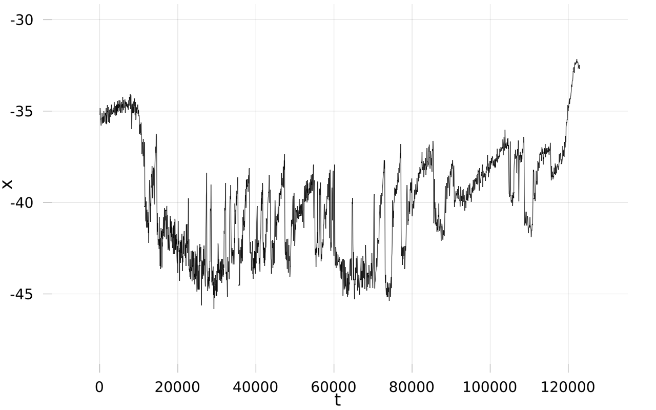
Refer to caption
Figure 3: NGRIP oxygen isotope δ18​O\delta_{18}\rm{O} measurements against time (years BP 2000).
Refer to caption
Figure 4: Realized quadratic variation process for NGRIP oxygen isotope δ18​O\delta_{18}\rm{O} measurements against time (years BP 2000).
Refer to caption
Figure 5: Shaded: marginal 90%90\,\%-posterior credible band for the piecewise constant posterior for the scale of the quadratic variation process of the ice core time series. Black: marginal posterior median.

6 Brief discussion of some extensions

In the treatment of our statistical problem the standing assumption so far was that observations were rooted in a model derived from (1), and that the process has been observed continuously in time. In an asymptotic setting we have derived contraction rates for the Bayesian estimator in Sections 3 and 4. There are (at least) two variations that immediately come to mind, an extended model that includes a drift component and a different observation regime, i.e. discrete time observations. We address these in the next two short sections and discuss how to adapt our previous statistical procedure to these situations.

6.1 Inclusion of drift

In principle, one could also consider a modification of the original SDE model by adding a drift,

Xt=∫0ta⁡(Xs)​𝑑s+∫0tσ⁡(Xs−)​d​Ls.X_{t}=\int_{0}^{t}a(X_{s})\,\mathrm{d}s+\int_{0}^{t}\sigma(X_{s-})\,\mathrm{d}L_{s}. (35)

The property that XX satisfying (35) has increasing paths is guaranteed by imposing that aa is nonnegative. Inclusion of the drift has the consequence that the laws of XX on [0,T][0,T] under presence and absence of a drift, but keeping the ∫0tσ⁡(Xs−)​d​Ls\int_{0}^{t}\sigma(X_{s-})\,\mathrm{d}L_{s} part the same for both cases, are automatically mutually singular. This happens because an absolutely continuous change of measure in this setting only changes the third characteristic of a semimartingale, which excludes a change of drift. This implies that the drift part, ∫0ta⁡(Xs)​𝑑s\int_{0}^{t}a(X_{s})\,\mathrm{d}s, can be identified with probability one.

Indeed, if XX is observed in continuous time, one also observes the process ∑s≤⋅ΔXs\sum_{s\leq\cdot}\Delta X_{s}, and therefore also the difference X−∑s≤⋅ΔXsX-\sum_{s\leq\cdot}\Delta X_{s}, which is ∫0⋅a⁡(Xs)​𝑑s\int_{0}^{\bm{\cdot}}a(X_{s})\,\mathrm{d}s. For the statistical problem of estimating σ\sigma, one can apply a modification of our procedure, by incorporating the values a⁡(Xs)a(X_{s}). For instance, if next to σ\sigma also aa is piecewise constant on bins, with known (or estimated) values aka_{k}, the assertion of Proposition 8 has to be modified by taking Δ​τ¯kn\Delta\bar{\tau}^{n}_{k} as n​Δ​bk​βα​σk+β​ak\frac{n\Delta b_{k}\beta}{\alpha\sigma_{k}+\beta a_{k}}. Hence we derive analogously to Theorem 11 that for any sequence mn→∞,m_{n}\to\infty,

Πn​(|ξk−σk|>mnn)→0​ in probability,\Pi_{n}\Bigl(|\xi_{k}-\sigma_{k}|>\frac{m_{n}}{\sqrt{n}}\Bigr)\to 0\mbox{ in probability},

for k=1,…,K,k=1,\ldots,K, where we model the (σk)(\sigma_{k}) as independent random variables (ξk)(\xi_{k}) and Πn\Pi_{n} stands for the posterior distribution of (ξk).(\xi_{k}).

6.2 Discrete time observations

In previous sections we have assumed that XnX^{n} given by (4) is observed continuously on a long time interval [0,Tn][0,T^{n}]. In this section the index nn plays no role (in the situation we will describe shortly, we even take n=1n=1 without loss of generality), it is fixed and therefore omitted below from our notation. The current setting is the practically relevant situation where XX is observed only discretely in time at timepoints t0,…,tmt_{0},\dots,t_{m}. We use the abbreviated notation Xd=(Xti)i=1mX^{d}=(X_{t_{i}})_{i=1}^{m}. It is assumed that realisations Xti=xtiX_{t_{i}}=x_{t_{i}}, i=0,…,mi=0,\dots,m have been observed. In this discrete time setting, the level hitting times τk\tau_{k}, are only known approximately: if bk∈[Xti,Xti+1)b_{k}\in[X_{t_{i}},X_{t_{i+1}}), then τk∈[ti,ti+1)\tau_{k}\in[t_{i},t_{i+1}). Our previous inference procedure for piecewise constant σ\sigma, assuming observation of the τk\tau_{k}, can then still be used in a data augmentation type Gibbs sampler, targeting the joint posterior distribution of XX and σ\sigma given the observations. The sampler alternates an interpolation step, where the random times τk\tau_{k} are sampled conditional on σ\sigma and the observations XtiX_{t_{i}}, and an inference step where σ\sigma is sampled conditional on the τk\tau_{k} as described before to obtain the posterior distribution. In this section we propose a procedure how to sample the τk\tau_{k} conditional on σ\sigma and observations XtiX_{t_{i}} to complement the continuous time inference procedure developed before, e.g. as in Section 3. For that extension, it is enough to assume that σ\sigma is a piecewise constant function, fixed and known. So we only consider the problem of sampling the posterior conditional on the observation of the process XtinX^{n}_{t_{i}} for piecewise constant σ\sigma given by (9). By the Markov property, the conditional distribution of XX given observations XdX^{d} factorises into independent distributions of the path of XX on time intervals [ti,ti+1)[t_{i},t_{i+1}). As the conditional distribution of σ\sigma only depends on the τk\tau_{k}, it is enough to sample the trajectory of XX on intervals [ti,ti+1)[t_{i},t_{i+1}) that are such that bk∈[Xti,Xti+1)b_{k}\in[X_{t_{i}},X_{t_{i+1}}) for some kk. We therefore concentrate on the task of sampling XX (for this purpose we can take n=1n=1 without loss of generality) conditional on XS=uX_{S}=u, XT=vX_{T}=v, S<TS<T with b=bk∈[u,v)b=b_{k}\in[u,v).

Simplifying, we assume that each bin contains at least one observation. Observe that if σ=1\sigma=1 then XtX_{t}, conditional on Xti=xtiX_{t_{i}}=x_{t_{i}}, Xti+1=xti+1X_{t_{i+1}}=x_{t_{i+1}} for ti<t<ti+1t_{i}<t<t_{i+1}, is just a gamma process bridge with known distribution. By Corollary 5 the law of the conditional process is absolutely continuous with respect the law of a conditional gamma process,

d​ℙTσd​ℙT1=exp⁡{β​∑k=1K[1−n​ξk−1]​(Xτk−Xτk−1)−α​∑k=1K(τk−τk−1)​log⁡(ξk/n)}.\displaystyle\frac{\mathrm{d}\mathbb{P}^{\sigma}_{T}}{\mathrm{d}\mathbb{P}^{1}_{T}}=\exp\left\{\beta\sum_{k=1}^{K}\left[1-n\xi_{k}^{-1}\right](X_{\tau_{k}}-X_{\tau_{k-1}})-\alpha\sum_{k=1}^{K}\left(\tau_{k}-\tau_{k-1}\right)\log(\xi_{k}/n)\right\}.

We denote the law of τ=(τ0,…,τK)\tau=(\tau_{0},\ldots,\tau_{K}) conditional on Xd=xdX^{d}=x^{d} by QτσQ^{\sigma}_{\tau}, emphasising the dependence on σ\sigma. By the abstract Bayes formula, it holds that, with the approximation below obtained by replacing XτkX_{\tau_{k}} with bkb_{k},

d​Qτσd​Qτ1​(τ0,…,τK)≈∏i=1mpσ​(ti−1,xti−1,ti,xti)p1​(ti−1,xti−1,ti,xti)​R​(τ0,…,τK)\frac{\mathrm{d}Q^{\sigma}_{\tau}}{\mathrm{d}Q^{1}_{\tau}}(\tau_{0},\dots,\tau_{K})\approx\prod_{i=1}^{m}\frac{p^{\sigma}(t_{i-1},x_{t_{i-1}};t_{i},x_{t_{i}})}{p^{1}(t_{i-1},x_{t_{i-1}};t_{i},x_{t_{i}})}R(\tau_{0},\dots,\tau_{K})

where pσ​(ti−1,xti−1,ti,xti)p^{\sigma}(t_{i-1},x_{t_{i-1}};t_{i},x_{t_{i}}) denotes the transition density of the process XX with volatility σ\sigma given Xti−1=xti−1X_{t_{i-1}}=x_{t_{i-1}} to the value Xti=xtiX_{t_{i}}=x_{t_{i}}, and

R⁡(τ0,…,τK)=exp⁡{β​∑k=1K[1−n​ξk−1]​(bk−bk−1)−α​∑k=1K(τk−τk−1)​log⁡(ξk/n)}.R(\tau_{0},\dots,\tau_{K})=\exp\left\{\beta\sum_{k=1}^{K}\left[1-n\xi_{k}^{-1}\right](b_{k}-b_{k-1})-\alpha\sum_{k=1}^{K}\left(\tau_{k}-\tau_{k-1}\right)\log(\xi_{k}/n)\right\}.

A random sample of τ\tau under Qτ1Q^{1}_{\tau} can be obtained, observing that the unnormalised density of τk\tau_{k} given Xti−1=xti−1X_{t_{i-1}}=x_{t_{i-1}} and Xti=xtiX_{t_{i}}=x_{t_{i}}, bk∈[xti,xti+1)b_{k}\in[x_{t_{i}},x_{t_{i+1}}) is approximately given by (τk\tau_{k} is now also used for a realisation of τk\tau_{k})

f⁡(τk)=p1​(ti−1,xti−1,τk,bk)​p1​(τk,bk,ti,xti)f(\tau_{k})=p^{1}(t_{i-1},x_{t_{i-1}};\tau_{k},b_{k})p^{1}(\tau_{k},b_{k};t_{i},x_{t_{i}})

with the approximation obtained by again replacing XτkX_{\tau_{k}} by bkb_{k}. So the posterior distribution of ξk\xi_{k} given Xd=xdX^{d}=x^{d} can be computed using a Gibbs type Metropolis-Hastings approach where in one step every τk\tau_{k} is sampled conditional on ξk\xi_{k} given Xd=xdX^{d}=x^{d} using Qτ1Q^{1}_{\tau} as proposal distribution with RR as (approximate) likelihood, and then in a next step, ξk\xi_{k} are sampled given τk\tau_{k} using (10).

6.3 More general driving processes

In this paper, we focus on SDEs with driving gamma processes. In principle, one can consider other driving Lévy processes, but then we will lose some nice features of the current model. The situation here is analogous to the diffusion case with Brownian noise. The Brownian noise enables one to write down a likelihood ratio ‘a la Girsanov. If one replaces the Brownian motion with an arbitrary continuous local martingale, the likelihood ratio will no longer be explicit. If one changes the gamma process to another increasing process in our setting, a similar phenomenon will arise. The exact expression of the likelihood ratio in Corollary 9 will change, and one has to use another prior instead of the inverse gamma one. Conceptually one can follow a similar strategy as we have proposed now, but a concrete realization will be different, and it is doubtful whether the explicit expressions for the likelihood and the posteriori distribution exist in this case.

Acknowledgments

The research leading to these results has received funding from the European Research Council under ERC Grant Agreement 320637. The research of the first author was supported by the HSE University Basic Research Program and the German Science Foundation research grant (DFG Sachbeihilfe) 406700014.

References

  • Batir (2008) Batir, N. (2008). Inequalities for the gamma function. Archiv der Mathematik, 91(6), 554–563.
  • Batz et al. (2018) Batz, P., Ruttor, A., & Opper, M. (2018). Approximate Bayes learning of stochastic differential equations. Phys. Rev. E, 98, 022109.
  • Belomestny et al. (2019) Belomestny, D., Gugushvili, S., Schauer, M., & Spreij, P. (2019). Nonparametric Bayesian inference for Gamma-type Lévy subordinators. Commun. Math. Sci., 17(3), 781–816.
  • Belomestny et al. (2021) Belomestny, D., Gugushvili, S., Schauer, M., & Spreij, P. (2021). Weak solutions to gamma-driven stochastic differential equations. In preparation.
  • Carson et al. (2019) Carson, J., Crucifix, M., Preston, S. P., & Wilkinson, R. D. (2019). Quantifying age and model uncertainties in palaeoclimate data and dynamical climate models with a joint inferential analysis. Proceedings of the Royal Society A: Mathematical, Physical and Engineering Sciences, 475(2224), 20180854.
  • Chance et al. (2008) Chance, D. M., Hillebrand, E., & Hilliard, J. E. (2008). Pricing an option on revenue from an innovation: An application to movie box office revenue. Management Science, 54(5), 1015–1028.
  • Ditlevsen (1999) Ditlevsen, P. D. (1999). Observation of α\alpha-stable noise induced millennial climate changes from an ice-core record. Geophysical Research Letters, 26(10), 1441–1444.
  • Dufresne et al. (1991) Dufresne, F., Gerber, H. U., & Shiu, E. S. W. (1991). Risk theory with the gamma process. ASTIN Bulletin, 21(2), 177–192.
  • Eguchi & Uehara (2020) Eguchi, S., & Uehara, Y. (2020). Schwartz type model selection for ergodic stochastic differential equation models. ArXiv, 1904.12398.
    URL https://arxiv.org/abs/1904.12398
  • Ghosal et al. (2000) Ghosal, S., Ghosh, J. K., & Van Der Vaart, A. W. (2000). Convergence rates of posterior distributions. Annals of Statistics, (pp. 500–531).
  • Ghosal & van der Vaart (2017) Ghosal, S., & van der Vaart, A. (2017). Fundamentals of nonparametric Bayesian inference, vol. 44 of Cambridge Series in Statistical and Probabilistic Mathematics. Cambridge University Press, Cambridge.
  • Gugushvili et al. (2020) Gugushvili, S., Mariucci, E., & van der Meulen, F. (2020). Decompounding discrete distributions: A non-parametric Bayesian approach. Scand J. Statist., 47(2), 464–492.
  • Gugushvili et al. (2019) Gugushvili, S., van der Meulen, F., Schauer, M., & Spreij, P. (2019). Nonparametric Bayesian volatility estimation. In J. de Gier, C. E. Praeger, & T. Tao (Eds.) 2017 MATRIX Annals, (pp. 279–302). Cham: Springer International Publishing.
  • Gugushvili et al. (2015) Gugushvili, S., van der Meulen, F., & Spreij, P. (2015). Nonparametric Bayesian inference for multidimensional compound Poisson processes. Mod. Stoch. Theory Appl., 2(1), 1–15.
  • Gugushvili et al. (2018) Gugushvili, S., van der Meulen, F., & Spreij, P. (2018). A non-parametric Bayesian approach to decompounding from high frequency data. Stat. Inference Stoch. Process., 21(1), 53–79.
  • Gushchin et al. (2019) Gushchin, A., Pavlyukevich, I., & Ritsch, M. (2019). Drift estimation for a Lévy-driven Ornstein-Uhlenbeck process with heavy tails. ArXiv, 1911.11202.
    URL https://arxiv.org/abs/1911.11202
  • Jasra et al. (2019) Jasra, A., Kamatani, K., & Masuda, H. (2019). Bayesian inference for stable Lévy–driven stochastic differential equations with high-frequency data. Scandinavian Journal of Statistics, 46(2), 545–574.
  • Jasra et al. (2011) Jasra, A., Stephens, D. A., Doucet, A., & Tsagaris, T. (2011). Inference for Lévy-driven stochastic volatility models via adaptive sequential Monte Carlo. Scandinavian Journal of Statistics, 38(1), 1–22.
  • Kabanov et al. (1986) Kabanov, Y. M., Liptser, R. S., & Shiryaev, A. (1986). On the variation distance for probability measures defined on a filtered space. Probability theory and related fields, 71(1), 19–35.
  • Koskela et al. (2019) Koskela, J., Spanò, D., & Jenkins, P. A. (2019). Consistency of Bayesian nonparametric inference for discretely observed jump diffusions. Bernoulli, 25(3), 2183–2205.
  • Kyprianou (2014) Kyprianou, A. E. (2014). Fluctuations of Lévy processes with applications. Introductory lectures. Universitext. Springer, Heidelberg, 2nd ed.
  • Müller & Mitra (2013) Müller, P., & Mitra, R. (2013). Bayesian nonparametric inference—why and how. Bayesian Anal., 8(2), 269–302.
  • Müller et al. (2015) Müller, P., Quintana, F. A., Jara, A., & Hanson, T. (2015). Bayesian nonparametric data analysis. Springer Series in Statistics. Springer, Cham.
  • Nickl & Söhl (2017) Nickl, R., & Söhl, J. (2017). Nonparametric Bayesian posterior contraction rates for discretely observed scalar diffusions. Ann. Statist., 45(4), 1664–1693.
  • North Greenland Ice Core Project Members (2007) North Greenland Ice Core Project Members (2007). 50 year means of oxygen isotope data from ice core NGRIP. Supplement to: North Greenland Ice Core Project Members (2004): High-resolution record of Northern Hemisphere climate extending into the last interglacial period. Nature, 431, 147-151, https://doi.org/10.1038/nature02805.
    URL https://doi.org/10.1594/PANGAEA.586886
  • Protter (2004) Protter, P. E. (2004). Stochastic integration and differential equations, vol. 21 of Applications of Mathematics (New York). Springer-Verlag, Berlin, 2nd ed. Stochastic Modelling and Applied Probability.
  • Reed & McKelvey (2002) Reed, W. J., & McKelvey, K. S. (2002). Power-law behaviour and parametric models for the size-distribution of forest fires. Ecological Modelling, 150(3), 239–254.
  • Silverman (1986) Silverman, B. W. (1986). Density estimation for statistics and data analysis. Monographs on Statistics and Applied Probability. Chapman & Hall, London.
  • Todorov (2011) Todorov, V. (2011). Econometric analysis of jump-driven stochastic volatility models. Journal of Econometrics, 160(1), 12–21.
  • Tsybakov (2008) Tsybakov, A. B. (2008). Introduction to nonparametric estimation. Springer Science & Business Media.
  • Uehara (2019) Uehara, Y. (2019). Statistical inference for misspecified ergodic Lévy driven stochastic differential equation models. Stochastic Processes and their Applications, 129(10), 4051–4081.
  • van Noortwijk (2009) van Noortwijk, J. (2009). A survey of the application of gamma processes in maintenance. Reliability Engineering & System Safety, 94(1), 2–21.
  • Wenocur (1989) Wenocur, M. L. (1989). A reliability model based on the gamma process and its analytic theory. Adv. in Appl. Probab., 21(4), 899–918.