Center of Poisson and skein algebras associated to loops on surfaces
Abstract.
We discuss and develop a systematic method to compute the Poisson center (Casimir) of various Poisson algebras associated to loops on orientable surfaces (possibly with boundary and punctures) introduced by Goldman and Wolpert in 80’s while studying Thurston’s earthquakes deformations. Our computation extends a result of Etingof to all finite type hyperbolic surfaces. We use these methods to compute the center of various skein algebras introduced by Turaev for the quantization of these Poisson algebras. As another application of our results we compute the center of homotopy skein algebra introduced by Hoste and Przytycki.
1. Introduction
Let be an oriented surface, possibly with boundary and punctures. We assume that the Euler characteristic of is negative so that admits a hyperbolic metric. We call such a surface a hyperbolic surface. We denote the fundamental group of by and the set of all free homotopy classes of oriented (respectively unoriented) closed curves in by (respectively ). Unless otherwise specified, we assume to be a commutative ring with identity containing the ring of integers . For any set , we denote by the free -module generated by .
In [12], Goldman discovered a Lie bracket on while studying the symplectic structure on the moduli space of representations of . The module with this Lie bracket is known as the Goldman Lie algebra which we denote by . He also showed that admits a natural Lie subalgebra on the submodule . This Lie subalgebra is known as the Thurston-Wolpert-Goldman Lie algebra which we denote by . See Section 2 for definitions and details.
Goldman’s work was inspired from the work of Wolpert ([24], [23]). In fact the Lie algebra was implicit in [24] (Wolpert called it twist lattice).
The symmetric algebras and of and respectively, admit natural Poisson algebra structures. If we allow Poisson algebras to be non-commutative then the universal enveloping algebras and also become Poisson algebras. Following Turaev, we (informally) call these Poisson algebras, the Poisson algebras of loops on .
In [22], Turaev introduced various skein algebras associated to the set of isotopy classes of links in the three manifold for the quantization of the Poisson algebras of loops. In [13], Hoste and Przytycki independently gave another quantization of the Poisson algebras of loops in terms of homotopy skein algebras. For recent development in the Poisson structure of the moduli space of representations and various skein algebras associated to them, see [19], [21], [20], [7], [16], [6], [5], [3], [18], [17].
The goal of this paper is twofold. Firstly to compute the Poisson center of the Poisson algebras of loops mentioned above. Secondly to use the quantizations of Turaev [22] and Hoste and Przytycki [13] to compute the center of various skein algebras.
Now we state the main results of the paper. The Poisson center , of a Poisson algebra is the subalgebra consists of elements such that for all . Elements of are also known as Casimir elements. The center plays an important role in the study of representations of .
In an earlier paper [9] with Moira Chas, the author computed the Poisson center of the Poisson algebras and . In the first main result of this paper we compute the Poisson center of the Poisson algebras and generalizing the result of Etingof [10] to all finite type hyperbolic surfaces.
Theorem.
For a hyperbolic surface , the Poisson center of the Poisson algebras and are generated by three types of homotopy classes of oriented curves: 1) constant curve, 2) curves homotopic to boundaries and 3) curves homotopic to punctures.
The above theorem naturally extends to the one parameter family of Poisson algebras associated to introduced by Turaev in [22, Section 2.2] (see Section 2.2).
The skein algebras associated to play a central role in the study of quantum invariants, topological quantum field theory and finite type invariants of links in -manifolds. In a series of papers [4], [5], [6] Bonahon and Wong studied the finite dimensional representations of the Kauffman bracket skein algebra which gave a quantization of the character variety. The central elements of Kauffman bracket skein algebra played a key role in their study and provided “classical shadow” invariant for the representations. Subsequently the center of the Kauffman bracket skein algebra was studied in [15], [18].
In [22], Turaev introduced quantization of Poisson algebras of loops in terms of Skein algebras , A(), and their quotients (see Section 7 and Section 8 for details). For oriented curves, the skein relations of these skein algebras are similar to the Jones-Conway skein relations. For unoriented curves, the skein relations are modified version of Kauffman bracket skein relations. In [13], Hoste and Przytycki gave another quantization of Poisson algebra of loops in terms of homotopy skein algebras and (see Section 9 for details). Our aim is to compute the centers of these skein algebras.
In that direction, the main results proved in the second part of the paper can be summarized in the following theorem.
Theorem.
The centers of the following skein algebras (over appropriate rings)
,, A()/ A(),
,
are generated by the empty link, the constant link and the links whose projection to are isotopic to the boundary components or punctures of .
As an application of our computation of Poisson centers we also obtain the following result.
Theorem.
The center of the homotopy skein algebra of oriented (respectively unoriented) links is generated by the empty link, the constant link and the oriented (respectively unoriented) links which are link homotopic to the boundary components or punctures of .
We further exploit the relation between these Poisson algebras and homotopy skein algebras to obtain various properties of these skein algebras.
1.1. Organization of the paper
In Section 2, we recall the definitions and properties of the Poisson algebras of loops introduced in [12] and related Poisson algebras introduced in [22] and [13]. In Section 3, we recall some basic facts about hyperbolic surfaces. In Section 4 we describe the geometry of the lifts of the terms of various Lie brackets of these Poisson algebras. In Section 5 we prove the main technical lemmas required for our proof. In Section 6 we compute the center of the Poisson algebras of loops. In Section 7,8 and 9 we define the various skein algebras and compute their centers. In Section 10 we explain a possible generalization of our theorems.
Acknowledgment
The author would like to thank Prof. Moira Chas for her encouragement and enlightening conversations.
2. Poisson algebras of loops
Let be a hyperbolic surface. We consider both oriented and unoriented closed curves on . Given an oriented curve we denote the corresponding unoriented curve by .
We fix an orientation on once and for all. All the pictures are drawn assuming the anti-clockwise orientation of the surface.
There is a one-to-one correspondence between the set of all free homotopy classes of oriented closed curves in and the set of all conjugacy classes in , both of which will be denoted by . The set of all free homotopy classes of unoriented closed curves will be denoted by .
We denote the free homotopy class of an oriented (respectively unoriented) closed curve (respectively ) by (respectively ).
We start with the definition of Goldman Lie algebra and Thurston-Wolpert-Goldman Lie algebra.
Definition 2.1.
Consider two oriented closed curves and in which intersect each other transversally in double points. Define the Goldman bracket between and by
where denotes the set of all intersection points between and , denotes the sign of the intersection between and at and is the loop product of and at . Extend the Goldman bracket to linearly.
Goldman [12] proved that the bracket is well defined on , is antisymmetric and satisfy Jacobi identity. Hence with the Goldman bracket forms a Lie algebra called the Goldman Lie algebra and it is denoted by . For convenience of notation we denote simply by .
Consider the involution defined by where denotes the same curve but with opposite orientation. The map extends linearly to a Lie algebra automorphism of . Therefore the stationary set is a Lie subalgebra of . The stationary set is canonically isomorphic to . We call this Lie subalgebra the Thurston-Wolpert-Goldman Lie algebra and denote it by
For an intrinsic definition of Thurston-Wolpert-Goldman Lie algebra see [9]. For convenience of notation we denote simply by .
Let be the universal enveloping algebra and be the symmetric algebra of . Similarly denote the universal enveloping algebra and symmetric algebra of by and respectively. For definition and basic properties of universal enveloping algebra and symmetric algebra see [1], [13].
A Poisson algebra over is an associative -algebra (possibly non-commutative) together with a Lie bracket that also satisfies Leibniz’s rule. The algebras and have natural Poisson algebra structures with the commutator being the Lie bracket. We extend the Lie bracket of and - using Leibniz rule - to and respectively. This make and Poisson algebras.
There are canonical maps from and to their corresponding universal enveloping algebra and symmetric algebra. To simplify notation, we denote an element and its image under these maps by the same notation. We also denote the product of two elements in these Poisson algebras simply by juxtaposing the elements.
Let us recall the Poincare-Birkhoff-Witt theorem for and (see [1], [13, Theorem 3.2]). We state it for . The statement for is exactly the same after you replace the oriented curves with their corresponding unoriented representatives.
Theorem 2.2.
Let be a fixed total order on . Consider the set
Both and are freely generated by as modules. Moreover the natural maps from into and are injective Lie algebra homomorphisms.
2.1. The algebras and
Let be any Lie algebra over . We recall the description of the algebra and its one parameter variants introduced by Turaev in [22, Section 1.3].
Let be the -module and be the tensor algebra of . The algebra is defined to be the quotient of by the two sided ideal generated by the relations . Therefore is an an associative algebra generated by .
Consider the Lie algebras and over , where we replace the Lie brackets by times the Goldman Lie bracket and Thurston-Wolpert-Goldman Lie bracket respectively. By [22, Remarks 2, Section 4.6], and are isomorphic to and respectively. Therefore (respectively ) is freely generated by the set (respectively the same set with oriented curves replaced by unoriented curves) in Theorem 2.2 as a module.
Turaev also considered the one parameter family of -algebras for any . When is a field and each is isomorphic to the algebra
2.2. A family of deformations of
Given any , we define by
for all , where is the algebraic intersection number between and . Extend to using bi-linearity and to using Leibniz rule. Then satisfy the Jacobi identity (see [22, Section 2.2]). We define the Poisson algebra over to be the -algebra with the Lie bracket . Observe that .
3. Hyperbolic geometry on surface.
In this section, we recall some basic results about hyperbolic geometry on surfaces. For the proofs of the results see [2], [11] and the references therein.
Let be an oriented surface of genus with boundary components and punctures. We assume the Euler characteristic of to be negative, i.e. . Every such surface admits a hyperbolic metric. We call an oriented surface with a given hyperbolic metric a hyperbolic surface.
Given any hyperbolic surface, we identify its universal cover with the hyperbolic plane and its fundamental group with a discrete subgroup of , the group of orientation preserving isometries of .
A closed curve is called essential if it is not homotopic to a point or to a puncture. It is called peripheral if it is homotopic to a puncture.
Given any essential oriented (respectively unoriented) closed curve in a hyperbolic surface, there is a unique oriented (respectively unoriented) geodesic in . Unless otherwise specified, we use the geodesic representatives from the corresponding free homotopy classes.
Recall that the Teichmüller space of is the set of all isotopy classes of marked hyperbolic surfaces where is a hyperbolic surface and is an orientation preserving diffeomorphism. Given any point , we associate a natural hyperbolic metric on , the pull back of the metric on by . We use this association to identify a point as a hyperbolic metric on . For ease of notation we sometimes denote simply by . Given any free homotopy class and any point , let be the length function, i.e., the length of the unique geodesic in in corresponding to the hyperbolic metric . We call a geodesic in the metric an -geodesic.
Let be a hyperbolic metric on and be two oriented -geodesics intersecting transversally at an intersection point . We define to be the angle at between the positive direction of and . To keep notations simple, we sometimes omit from the notations of angle and length. The meaning should be clear from the context.
Given two closed curves and , the geometric intersection number between and is defined to be The following lemma is a well known result.
Lemma 3.1.
Let be an orientable surface and be a closed curve on such that for every simple closed curve . Then is either homotopically trivial or homotopic to a boundary curve or homotopic to a puncture.
4. Lift of the loop products to
In this section we discuss the geometry of loop product described in the definition of Goldman Lie bracket. For details see [8], [14].
We fix a metric . We discuss all geometric objects, lengths and angles with respect to without mentioning it explicitly. We identify the universal cover of (with metric ) to . Unless otherwise mentioned, in this section, we assume all geodesics to be oriented.
Let and be two oriented geodesics in and be a transverse intersection double point between them. We call any oriented lift of a geodesic to an axis of . We use the notation for a generic axis of and for an axis of passing through a point . Our starting point is the following result to find an axis and the length of the geodesic in .
Let be any lift of to . There exist two lifts and of and respectively, intersecting at (see Figure 1). Let be the point on at a distance from in the forward direction of and be the point on at a distance from in the backward direction of .

Theorem 4.1.
[2, Theorem 7.38.6] With the above notation, the geodesic containing the geodesic segment from to (with orientation from to ) is an axis of the geodesic in . We also have
Construction of a lift
We recall the construction of a lift of from [8, Section 7]. Let be a lift of . To construct a lift of passing through , we do the following (see Figure 2). First consider the geodesic axis of . Travel the length , from , in the forward direction along to reach the point . Now from travel the distance along to reach . We continue the same process from and repeat it indefinitely. Similarly we do the same construction from in backward direction. The construction yields a lift of which is a bi-infinite piecewise geodesic whose geodesic pieces are consecutive geodesic arcs of axes of and of length and respectively.

Let be the midpoint of and for all . Then by Theorem 4.1, there exists an axis of which passes through ’s. We use the notation and for a generic lift of and its axis obtained from the above construction. We call the geodesic arcs of corresponding to axes of and as -pieces and -pieces respectively. Therefore any lift obtained from the above construction is an oriented piecewise geodesic where the geodesic pieces are -pieces and -pieces appearing alternatively. Unless otherwise mentioned, by a lift of we mean a lift obtained by the above construction.
Lemma 4.2.
Let be a lift of and be its axis. Consider any two consecutive -pieces (respectively -pieces) of and let and be the intersection points between these pieces and . Then the distance between and is Moreover there exist a -piece (respectively -piece) which intersects at which is the midpoint of and
5. Technical lemmas
In this section we prove the key lemmas that we use for proving our theorems. We prove them separately because they might be of independent interest.
Lemma 5.1.
Let and be three pairwise distinct oriented -geodesics such that is simple. Let and such that and be any positive integer. Consider any two lifts and of and respectively. Suppose and have the same axis . Then for any -piece of and any -piece of , we have .
Proof.
As is simple any two distinct geodesic lifts of are disjoint. Therefore any two -pieces are either disjoint or intersect in a geodesic segment.
If possible suppose and intersect in a geodesic segment. By the construction intersects both and at their midpoints. Hence . By the assumption . Therefore - by construction - the -piece of occurring immediately after coincides with the -piece of occurring immediately after . This implies tha an axis of coincides with an axis of and , which contradicts the fact that the geodesics and are distinct. ∎
Lemma 5.2.
Let and and be three oriented -geodesics. Let be an intersection point between and and be an intersection point between and . Suppose for two distinct positive integral values of . Then for any , and .
Proof.
Fix any arbitrary metric . To simplify notation throughout the proof we measure lengths and angles with respect to without mentioning it explicitly. Observe that the equality is topological.
Now for all positive integer . As , the geodesics corresponding to the two free homotopy classes are the same. Hence for two distinct values of . Therefore by Theorem 4.1,
This implies
The left hand side of the equation depends on but the right hand side is independent of . Hence as the equality holds for two distinct values of , Therefore and .
∎
Lemma 5.3.
Let and and be three oriented -geodesics such that is simple. Let be an intersection point between and and be an intersection point between and . Suppose for two distinct positive integral values of . Then .
Proof.
Lemma 5.4.
Let and and be three pairwise distinct oriented -geodesics. Let be an intersection point between and and be an intersection point between and such that . Suppose and is simple. If for any positive integer , then one of the following is true:
1) either there exist such that ,
2) or there exist such that .
Proof.
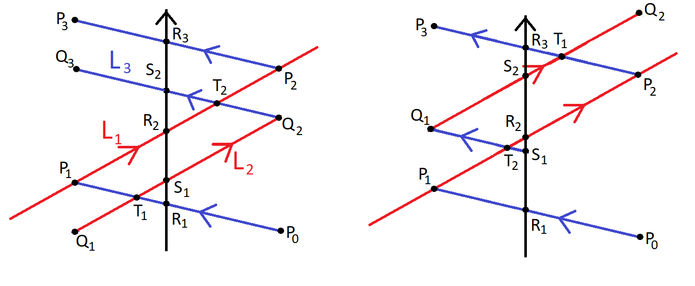
We prove the result for . The angle at any intersection point between and is same as the angle at between and as they are physically the same point. Combining the last statement with the equality , the proof for follows by a similar argument.
Without loss of generality assume . Fix a lift of (see Figure 3). As , both free homotopy classes have the same geodesic representative. Therefore . As , by Theorem 4.1, Also there exists a lift of such that . We denote simply by and the length of an arc by .
Choose a segment of consisting of two consecutive -pieces and and an -piece between them. Let for . By Lemma 4.2, .
By the construction of , there exist an -piece of which intersects in the arc . There are two possibilities: Case (a) intersects in or Case (b) intersects in
Case (a) intersects in : Consider left hand side picture of Figure 3. Let be the -piece in occurring immediately after . Let and be the geodesics in containing and respectively. As is simple, either or . If then . Which implies coincides with , contradicting Lemma 5.1. Therefore , in particular . Consider the geodesic triangle . As intersects but does not intersect , must intersect . Denote the intersection point of and by . By construction, intersects in . Therefore must intersect . Denote the intersection point between and by . Let be the projection of on for . Then and . Consider the geodesic quadrilateral . We have . Now , and . Therefore we have which proves the claim.
Case (b) intersects in : Consider right hand side picture of Figure 3 (right)). In this case we have to consider the -piece in occurring before . By the same argument as above we get two points and their projections and with the desired property. ∎
6. Universal enveloping algebra and symmetric algebra
Theorem 6.1.
The Poisson center of the Poisson algebras and are generated by scalars , the free homotopy class of constant curve and the curves homotopic to boundaries and punctures.
Proof.
Fix a metric and choose to be any simple -geodesic. Throughout the proof we consider -geodesic representatives of each curve. First we prove the result for . Let be an element of the center of . Then by Theorem 2.2,
where for all . We have
Denote by , the set of all intersection points between and for all . Consider such that for all . Let .
As is commutative, we can rearrange the terms in ascending order with respect to and assume they are elements of the set of Theorem 2.2.
As for all positive integer , from the above expression and Theorem 2.2, there exists such that one of the following is true for all but finitely many positive integers .
- •
- •
. This is impossible by Theorem 4.1 because the left hand side depends on but the right hand side is independent of .
Therefore each is disjoint from . As is an arbitrary simple closed geodesic, each is disjoint from every simple closed geodesic on the surface. Hence by Lemma 3.1 each is either a constant loop or a loop homotopic to a puncture or a loop homotopic to a boundary component.
Now we prove the result for . Let be the tensor algebra of . Let be the ideal generated by the elements of the form , where is any positive integer and . Then .
Let be the ideal generated by the elements of the form . Then .
Let be the canonical map. By Theorem 2.2, is a module isomorphism.
We have a action on obtained by extending the adjoint action of on itself by derivations. For we denote the action on by .
On the other hand also acts on by the following:
A straightforward computation shows, for all As the center of is exactly and the center of is exactly , the center of and are the same. Therefore the result follows from the first part.
∎
The corresponding theorem for was proved in [9].
Theorem 6.2.
[9, Poisson Center Theorem] The Poisson center of the Poisson algebras and are generated by scalars , the free homotopy class of constant curve and the curves homotopic to boundaries and punctures.
Corollary 6.3.
The center of and are generated by scalars , the free homotopy class of constant curve and the curves homotopic to boundaries and punctures. If is a field and then the same result holds true for and .
7. Skein algebras of oriented curves
Consider the three manifold . A knot in a three manifold is a smooth embedding of in the interior of the three manifold. A link in a three manifold is a disjoint finite collection of knots. We also include the empty set as a unique link up to isotopy. Given any link we denote the number of components of by .
A triple of links is called a Conway triple if they are identical outside a ball and inside the ball they appear as shown in Figure 4. The crossing inside the ball can be one of two types: (1) mutual crossing between two components or (2) self crossing of a component. For type (1), we have and for type (2) we have .

The skein module is a module over the polynomial ring defined as follows. Suppose be the set of all isotopy classes of oriented links in . Then is the quotient of the free -module generated by by the submodule generated by the following relations.
(i) For Conway triple with crossing type (1) we have the relation
(ii) For Conway triple with crossing type (2) we have the relation
7.1. Algebra structure on
We fix the product orientation on We define the product of two links and to be the link obtained by stacking above . This product induces an associative algebra structure in with the class of empty set being identity.
7.2. Skein algebra A()
The skein algebra A() is defined to be the quotient of by the ideal . Therefore A() is an associative algebra over the polynomial ring .
Theorem 7.1.
The center of the skein algebra A()/ A() over is generated by the empty link, the constant link and the links which are isotopic to the boundary components or punctures of .
Theorem 7.2.
The center of the skein algebra over is generated by the empty link, the constant link and the links which are isotopic to the boundary components or punctures of .
Theorem 7.3.
The center of the skein algebra over is generated by the empty link, the constant link and the links which are isotopic to the boundary components or punctures of .
8. Skein algebras of unoriented curves
Let be the commutative ring Consider the three manifold . Let be the set of all regular isotopy classes of unoriented link diagrams. Recall that the regular isotopy is the equivalence relation in the link diagrams generated by 2nd and 3rd Reidemeister moves only. We denote the number of components of a link diagram by .
The skein module is a module over which is defined to be the quotient of the free -module generated by by the submodule generated by the following relations.
i)
where are arbitrary set of four non-empty link diagrams which are identical except in the neighbourhood of one crossing where they appear as shown in Figure 6 (replace by ).
ii) , where and are arbitrary pair of non-empty link diagrams which are identical except in the neighbourhood of one crossing where they appear as shown in Figure 5.
iii) , where denotes the link diagram of the trivial knot and denotes the link diagram of the empty link.

As in the oriented case, we define the product structure on by stacking one link over another which makes an associative algebra.
Theorem 8.1.
The center of the skein algebra over is generated by the empty link, the constant link and the links which are isotopic to the boundary components or punctures of .
Theorem 8.2.
The center of the skein algebra over is generated by the empty link, the constant link and the links which are isotopic to the boundary components or punctures of .
9. Homotopy skein algebras of
In [13], homotopy skein modules for 3-manifolds were introduced. In this section, we recall its definition and its relation with Goldman Lie algebras and . For this section we assume to be , the integral polynomial ring in variable .
Two links are said to be link homotopic in if one can be deformed to another by isotopy and componentwise homotopy, i.e. each component is allowed to cross itself but crossing between two distinct component is not allowed.
Let (respectively ) be the set of all link homotopy classes of oriented (respectively unoriented) links in , including the empty link. Let (respectively ) the free module generated by (respectively ).

Suppose and are three oriented links which are identical outside a ball and inside the ball they look as in Figure 4. Also assume that the two arcs belong to two different components. Let be the submodule of generated by all the relations of the form . We define the homotopy skein module to be
Similarly suppose and are four unoriented links which are identical outside a ball and inside the ball they look as in Figure 6. Also assume that the two arcs belong to two different components. Let be the submodule of generated by all the relations of the form . We define the Kauffman homotopy skein module to be
As before, the modules and admit a natural algebra structure from stacking product. Let and be two oriented (respectively unoriented) links. Define the stacking product to be the link obtained by placing above (i.e. and ).
Consider the Lie brackets and in and respectively. Let (respectively be the Lie algebra (respectively ) with the Lie bracket (respectively ). It is clear that both (respectively and (respectively have the same center.
Theorem 9.1.
The center of (respectively ) is generated by the empty link, the constant link and the oriented (respectively unoriented) links which are link homotopic to the boundary components or punctures of .
10. Observations
By [12, Theorem 5.4 and Theorem 5.13], we can treat the elements of and as classical observables on the moduli space of representations. By the results of [22] and [13] we can treat the elements on various skein algebras discussed earlier as quantum observables. The degeneration from quantum objects to classical object is simply the natural projection of the links in to curves in .
For this discussion, we fix a metric in and consider geodesics with respect to this metric without specifying it explicitly. Given an isotopy class of a link , we denote its representative in by . Given any link and a crossing of crossing type , let be the element in which is the term corresponding to the symbols or in Figure 4 depending on whether is or . Given crossings of of crossing type and symbols define inductively. We call the crossings of Figure 4 associated with the symbol and as the crossings of type and respectively.
Let be the projection map. Given two elements , choose representatives and such that and are geodesics in . Let be the mutual crossings between and of type and be the mutual crossings between and of type . Therefore we use the relation associated to Conway Triples with crossing type (1) at these crossings to get the following. Let .
Let and . Then
But Putting the values of and in the equation we get
By [22, Lemma 4.3], and .
If we choose such that for some simple closed curve then by the proof of Theorem 6.1, for sufficiently large , the links are pairwise non isotopic as the curves are pairwise not freely homotopic to each other. Therefore a necessary condition for the center of or any of its quotient to have elements in the Poisson center different from the classical one is that the elements corresponding to must be related to each other via the skein relations. In other words if the skeins appearing on the right hand side of the above equation are linearly independent in or any of its quotients then their Poisson centers are the algebra generated by links isotopic to boundary or punctures. The process also works in case of skein algebras of unoriented loops.
References
- [1] Eiichi Abe, Hopf algebras, vol. 74, Cambridge University Press, 2004.
- [2] Alan F Beardon, The geometry of discrete groups, vol. 91, Springer Science & Business Media, 2012.
- [3] Francis Bonahon and Xiaobo Liu, Representations of the quantum Teichmüller space and invariants of surface diffeomorphisms, Geom. Topol. 11 (2007), 889–937. MR 2326938
- [4] Francis Bonahon and Helen Wong, Representations of the Kauffman bracket skein algebra I: invariants and miraculous cancellations, Invent. Math. 204 (2016), no. 1, 195–243. MR 3480556
- [5] by same author, Representations of the Kauffman bracket skein algebra II: Punctured surfaces, Algebr. Geom. Topol. 17 (2017), no. 6, 3399–3434. MR 3709650
- [6] by same author, Representations of the Kauffman bracket skein algebra III: closed surfaces and naturality, Quantum Topol. 10 (2019), no. 2, 325–398. MR 3950651
- [7] Laurent Charles and Julien Marché, Multicurves and regular functions on the representation variety of a surface in su (2), arXiv preprint arXiv:0901.3064 (2009).
- [8] Moira Chas and Siddhartha Gadgil, The extended Goldman bracket determines intersection numbers for surfaces and orbifolds, Algebraic & Geometric Topology 16 (2016), no. 5, 2813–2838.
- [9] Moira Chas and Arpan Kabiraj, The lie bracket of undirected closed curves on a surface, to appear in Trans. Amer. Math. Soc., arXiv:1910.08991 (2020).
- [10] Pavel Etingof, Casimirs of the Goldman lie algebra of a closed surface, International Mathematics Research Notices 2006 (2006), no. 9, 24894–24894.
- [11] Benson Farb and Dan Margalit, A primer on mapping class groups, Princeton Mathematical Series, vol. 49, Princeton University Press, Princeton, NJ, 2012. MR 2850125
- [12] William Goldman, Invariant functions on Lie groups and Hamiltonian flows of surface group representations, Inventiones Mathematicae 85 (1986), no. 2, 263–302.
- [13] Jim Hoste and Jósef H Przytycki, Homotopy skein modules of orientable 3-manifolds, Mathematical Proceedings of the Cambridge Philosophical Society, vol. 108, Cambridge University Press, 1990, pp. 475–488.
- [14] Arpan Kabiraj, Center of the Goldman Lie algebra, Algebraic & Geometric Topology 16 (2016), no. 5, 2839–2849.
- [15] Thang T. Q. Lê, On Kauffman bracket skein modules at roots of unity, Algebr. Geom. Topol. 15 (2015), no. 2, 1093–1117. MR 3342686
- [16] Julien Marché, The Kauffman skein algebra of a surface at , Mathematische Annalen 351 (2011), no. 2, 347–364.
- [17] Julien Marché and Christopher-Lloyd Simon, Valuations on the character variety: Newton polytopes and residual poisson bracket, arXiv preprint arXiv:2104.04340 (2021).
- [18] Józef H. Przytycki and Adam S. Sikora, Skein algebras of surfaces, Trans. Amer. Math. Soc. 371 (2019), no. 2, 1309–1332. MR 3885180
- [19] Vladimir Turaev, Loops in surfaces and star-fillings, arXiv preprint arXiv:1910.01602 (2019).
- [20] by same author, Quasi-Poisson structures on moduli spaces of quasi-surfaces, Journal of Geometry and Physics (2020), 103743.
- [21] by same author, Topological constructions of tensor fields on moduli spaces, Advances in Mathematics 392 (2021), 107998.
- [22] by same author, Skein quantization of Poisson algebras of loops on surfaces, Annales scientifiques de l’Ecole normale supérieure, vol. 24, 1991, pp. 635–704.
- [23] S Wolpert, The Fenchel-Nielsen deformation, Annals of Mathematics (1982).
- [24] Scott Wolpert, On the symplectic geometry of deformations of a hyperbolic surface, Ann. of Math.(2) 117 (1983), no. 2, 207–234.