Excitation of Zonal Flow by Intermediate-Scale Toroidal Electron Temperature Gradient Turbulence

Recently, large-box-size, long-time-scale gyrokinetic simulations have been carried out to investigate the toroidal electron temperature gradient (ETG) driven turbulence parker; howard16; colyer; holland17. It is found that, unlike the usual theoretical expectations kim03; lin05; chen05, the formation of zonal flow (ZF) can play an important role in regulating intermediate-scale ETG turbulence and become dominant in the final saturation. Since the long-time saturated state is more experimentally relevant, ETG-ZF dynamics is crucial for understanding the nonlinear ETG physics and associated turbulent transport. In this work, motivated by the simulation observations, we present a gyrokinetic analysis addressing the spontaneous and forced ZF generation on the same footing. Our results indicate that the ETG nonlinearity is of a Navier-Stokes form at intermediate-scales, which is generally much stronger than the Hasegawa-Mima type nonlinearity in fluid limit lin05; chen05, and, thus, a significant ZF generation is expected for intermediate-scale toroidal ETG turbulence.

For simplicity and clarity, we consider an axisymmetric, low-$\beta$ (plasma to magnetic pressure), large aspect-ratio ($\epsilon=r/R_{0}\ll 1$) tokamak with the usual minor radius ($r$), poloidal ($\theta$) and toroidal ($\zeta$) coordinates. We examine a single high-$n$ ETG mode and associated zonal flow. Adopting ballooning representation connor78, the ETG fluctuation can be written as

where the subscript $\bm{k}\equiv(n,\theta_{k})$ denotes the wavenumber space, and $nq^{\prime}\theta_{k}$ is a radial envelope wavenumber with $q(r)$ being the safety factor.

The analysis presented here will focus on intermediate-scale turbulence with $k_{\perp}^{2}\rho_{e}^{2}\ll 1\ll k_{\perp}^{2}\rho_{i}^{2}$, where the Debye shielding is negligible, and the ETG mode is nearly isomorphic to its ion-scale counterpart ITG mode, except for the ion adiabatic response for both ZF and ETG. We can therefore impose the quasineutrality condition

where $\tau=T_{e}/T_{i}$ is the temperature ratio, $J_{\bm{k}}=J_{0}(k_{\perp}\rho_{e}v_{\perp})$ is the zeroth-order Bessel function accounting for the finite Larmor radius (FLR) effect, and $\delta H_{\bm{k}}$ can be derived from the nonlinear gyrokinetic equation frieman:

Here, we have normalized the electrostatic potential as $\Phi_{\bm{k}}=e\delta\phi_{\bm{k}}/(\rho_{*}T_{e})$ with $\rho_{*}=\rho_{e}/r_{n}$, and defined the Poisson bracket $[A,B]=(\partial_{\theta}A/r)\partial_{r}B-(\partial_{r}A)\partial_{\theta}B/r$. $\mathcal{L}_{\bm{k}}=[i\partial_{t}+\omega_{t}+\omega_{d}]$ is the inverse phase-space linear propagator, where $\omega_{t}=v_{te}v_{\parallel}(nq+i\partial_{\theta})/(qR_{0})$ and $\omega_{d}=(v_{\parallel}^{2}+v_{\perp}^{2}/2)v_{te}^{2}(i\sin\theta\partial_{r}-k_{\theta}\cos\theta)/(|\omega_{ce}|R_{0})$ denote, respectively, the transit and magnetic drift frequencies. $\omega_{*e}=k_{\theta}cT_{e}/(eBr_{n})$ is the electron diamagnetic drift frequency, $\omega_{*e}^{t}=-\omega_{*e}[1+\eta_{e}(v^{2}-3/2)]$ and $\eta_{e}=r_{n}/r_{ti}$, with $k_{\theta}=m/r$, and $r_{n}$ and $r_{t_{i}}$ being, respectively, the equilibrium density and temperature scale lengths. $F_{0}$ is the local Maxwellian. $\bm{k}_{2}$ satisfies the matching conditions $\bm{k}=\bm{k}_{1}-\bm{k}_{2}$.

In ballooning space, it is well known that the dominant order linear gyrokinetic equation is an ordinary differential equation parameterized by $\theta_{k}$. To allow a tractable weak turbulence analysis, we assume a local kinetic model kim to capture essential linear properties of toroidal ETG mode. In particular, we replace the $\eta$ variable by its parallel-mode-structure-averaged value $\bar{\eta}=[\int d\eta\tilde{\Phi}^{*}\eta^{2}\tilde{\Phi}]^{1/2}$. The linear dispersion relation then reduces to an algebraic equation

where $\omega_{t}=-v_{te}v_{\parallel}/(qR_{0}\bar{\eta})$ and $\omega_{d}=-\omega_{*e}\epsilon_{n}(2v^{2}_{\parallel}+v^{2}_{\perp})[s(\bar{\eta}-\theta_{k})\sin\bar{\eta}+\cos\bar{\eta}]$, with the magnetic shear $s=rq^{\prime}/q$ and $\epsilon_{n}=r_{n}/R_{0}$. $\langle\cdots\rangle_{v}\equiv\int d\bm{v}(\cdots)$ and the $r$ dependency corresponds to equilibrium variations, As an example, the normalized linear ETG spectrum $\Omega_{\bm{k}}=\omega_{\bm{k}}/|\omega_{*e}|$ for typical tokamak plasma parameters is plotted in Fig. (1).

The nonlinear description of ZF can be obtained by taking neoclassical effects into account rosenbluth; kim03, yielding

where the length and time scales are normalized to $\rho_{e}$ and $|\omega_{*e}^{-1}|$, respectively. We have added an ad hoc gyrodiffusive contribution ($\propto d_{z}$) to the ZF collisional damping rate, of which the importance has been emphasized previously ricci. $\gamma_{z}\simeq 3\nu_{ee}/(|\omega_{*e}|\sqrt{\epsilon})$ with $\nu_{ee}$ being the electron-electron collision frequency, and $\chi_{z}=\tau+(1+1.6q^{2}/\sqrt{\epsilon})k_{\theta}^{2}\rho_{e}^{2}s^{2}\theta_{k}^{2}/2$ is the total susceptibility kim03. The nonlinear term arises from Reynolds stress, where we defined a parallel decoupling function $a_{n}=a_{n}(\theta_{k},\vartheta_{k})=\int d\eta\langle\tilde{\Phi}^{*}_{n}(\eta,\vartheta_{k})v_{\perp}^{2}\delta\tilde{H}_{n}(\eta,\vartheta_{k}+\theta_{k})\rangle_{v}$ to measure the parallel correlation of ETG turbulence, and it can limit the nonlinearity via the finite localization of linear parallel mode structures. As a simple but relevant paradigm, we assume $a_{n}=a_{n}(0,0)\textrm{exp}(-\theta_{k}^{2}/2\bar{\eta}^{2})$ in the present study, which essentially treats $\theta_{k}$ as a tilting angle sugama; chen18.

Solving Eq. (2) to the next order, the quasineutrality condition straightforwardly produces the following nonlinear Schrödinger equation for the ETG amplitude,

Here, $\gamma_{n}$ is the linear growth rate, $b_{n}k_{\theta}^{2}\rho_{e}^{2}s^{2}\theta_{k}^{2}$ denotes the frequency mismatch, and the $\propto c_{n}$ term recovers the correction associated with the plasma nonuniformities in real space. The parameters $b_{n}=-(\partial_{\theta_{k}}^{2}D_{\bm{k}}/\partial_{\Omega_{\bm{k}}}D_{\bm{k}})/(2k_{\theta}^{2}\rho_{e}^{2}s^{2})$ and $c_{n}=(\partial_{r}^{2}D_{\bm{k}}/\partial_{\Omega_{\bm{k}}}D_{\bm{k}})/2$ are determined by linear ETG dynamics. The nonlinear term, meanwhile, is the coupling of ZF to ETG mode via $E_{r}$ shearing. One readily identifies that, the ETG saturation is set by competition between linear growth and ZF-induced scattering to the linearly stable short radial wavelengths.

Equations (4) and (5), along with the complex parameters solely by linear ETG properties, fully characterize the dynamics of coherent ETG-ZF system, and will hereafter be referred to as the nonlinear Schrödinger equation (NLSE) model. To properly account for the kinetic effects, the conventional fluid limit is not assumed here, while both the forced and spontaneous generation of ZF are kept on the equal footing. We emphasize that the coupling of ZF to ETG is formally of Hasegawa-Mima type in the fluid limit hasegawa; chen05, and is $\mathcal{O}(k_{\theta}^{2}\rho_{e}^{2})$ weaker than the Navier-Stokes type nonlinearity in the present gyrokinetic analysis. As a consequence, ZF can more easily regulate the underlying ETG turbulence, and it will be shown later that the threshold condition for spontaneous ZF excitation is reduced by a factor $\mathcal{O}(k_{\theta}^{2}\rho_{e}^{2})$ relative to previous fluid prediction.

It is illuminating to notice that a four-wave model chen00 can be straightforwardly extracted from the NLSE model. By ignoring plasma nonuniformities and assuming the narrow-band ZF and ETG amplitudes, respectively, as $A_{z}\Pi[(\theta_{k}-\theta_{z})/W]$ and $A_{0}\Pi(\theta_{k}/W)+A_{+}\Pi[(\theta_{k}-\theta_{z})/W]+A_{-}\Pi[(\theta_{k}+\theta_{z})/W]$, one readily obtains

and

Here, $\Pi$ is the usual rectangle function, $W$ explicitly denotes the bandwidth, $k_{z}=k_{\theta}s\theta_{z}$ is the radial wavenumber, and $A_{0}$ and $A_{\pm}$ are, respectively, the pump ETG mode and sidebands produced by the envelope modulation. $\Delta=\textrm{Re}(b_{n})k_{z}^{2}\rho_{e}^{2}$ is the frequency mismatch and $\gamma_{s}=\gamma_{n}+\textrm{Im}(b_{n})k^{2}_{z}\rho_{e}^{2}$ is the linear growth/damping rate of sidebands. The four-wave model has the following the conservation property

The four-wave model is a dynamical system that displays both weak and strong nonlinear behaviours. We first explore the onset condition of the modulational instability with a constant pump amplitude $A_{0}$. In this case, the system is linear and a dispersion relation can be derived from Eqs. (6)-(8), by letting $\partial_{t}\equiv\Gamma_{z}$, as

which gives the critical threshold condition:

Thus, as discussed earlier, the threshold pump wave intensity is much lower (an order $\mathcal{O}(k_{\theta}^{2}\rho_{e}^{2})$) than the value from fluid theory chen05. Moreover, after some straightforward algebra, one can show that the threshold $|A_{0,c}|^{2}$ is minimized at $\theta_{z,m}^{2}\simeq 4\bar{\eta}^{2}/\{1+[1+4\kappa^{2}d_{z}+4\kappa^{4}(1+1.6q^{2}/\sqrt{\epsilon})(d_{z}+1/\kappa^{2})/\tau]^{1/2}\}$, with $\kappa^{2}=2k_{\theta}^{2}\rho_{e}^{2}s^{2}\bar{\eta}^{2}$. For typical tokamak parameters, as shown in Fig. (2), ZFs are more easily excited around $|\theta_{z,m}|\sim\mathcal{O}(1)$, and the growth rate above the critical amplitude threshold, meanwhile, peaks at $|\theta_{z}|\gtrsim|\theta_{z,m}|$. The ETG-ZF interactions, thereby, tend to ultimately isotropize the linear streamers. These effects are mainly attributed to the parallel decoupling between the pump and sidebands in Reynolds stress term, rather than the gyrodiffusive correction.

Next, consider the temporal evolution of the four-wave model. From Eq. (10), one can easily show that explosive growth exists for $\gamma_{n},\gamma_{s}>0$. On the other hand, for $\gamma_{n}+\gamma_{s}<0$, we can demonstrate, by using Eqs. (6)-(9), that the four-wave model gives a fixed-point solution with a constant $A_{z}$ for sufficiently low ZF damping rate, namely,

and

where $\delta=\Delta\gamma_{n}/(\gamma_{s}+\gamma_{n})$ is the amplitude oscillation frequency of ETGs due to their nonlinear interplay with the ZF. That is, the ETG turbulence is still fluctuating as the ZF converges to a steady-state, consistent with recent numerical results colyer. It also follows from Eqs. (13) and (14) that, as in the case of ITG turbulence diamond98, $|A_{0,p}|^{2}$ is proportional to the ZF collisional damping, while the ZF level is $\gamma_{z}$ independent. However, it is important to note that the estimate of the saturated ETG fluctuation level given by Eq. (14) is only valid for the four-wave model with a single ZF mode. For any realistic system with a spectrum of radial ZF modes, the ETG turbulence will subsequently continue driving ZF with lower threshold condition. Thus, one may use the $|A_{0,p}|^{2}$ value at $\theta_{z}=\theta_{z,m}$ to quantitatively estimate the ETG saturation level.

The NLSE model is of integrodifferential nature and generally requires numerical solution. Figure (3) shows the typical time histories for the averaged amplitude $\langle|A_{j}|\rangle=(\int d\theta_{k}|A_{j}|^{2})^{1/2}$ and dimensionless radial wavenumber $\langle|\theta_{j}|\rangle=(\int d\theta_{k}\theta_{k}^{2}|A_{j}|^{2})^{1/2}/\langle|A_{j}|\rangle$ of the ETG and ZF. One can identify that three stages of the nonlinear evolution of NLSE model. The first stage is early on before the global ETG mode structure is formed. Although the ZF is being force driven, its spectrum is very sensitive to the specific initial conditions for the ETG and thereby unpredictable. In the second stage, a global ETG linear mode structure has already been formed, but the ETG nonlinearity is still negligible. In this case, the ZF spectrum can be analytically evaluated as

where $\sigma^{2}=-b_{n}/4c_{n}$, $\delta\Omega=i\gamma_{n}-2c_{n}\sigma$ and $\gamma_{g}=\textrm{Im}(\delta\Omega)$ is the growth rate of the global linear ETG with $A_{n,f}=A_{n,0}\textrm{exp}(-\sigma k_{z}^{2}\rho_{e}^{2}-i\delta\Omega t)$. The defining feature of the force-driven process, i.e., an $\textrm{exp}(2\gamma_{g}t)$ factor, is readily recognized. It is worthwhile mentioning that, although the spectral shape is deterministic, the ZF intensity will depend on initial conditions. Figure (4) shows that the predicted ETG-ZF spectral shapes at the force-driven stage ($t=69$) are in qualitative agreement with numerical results.

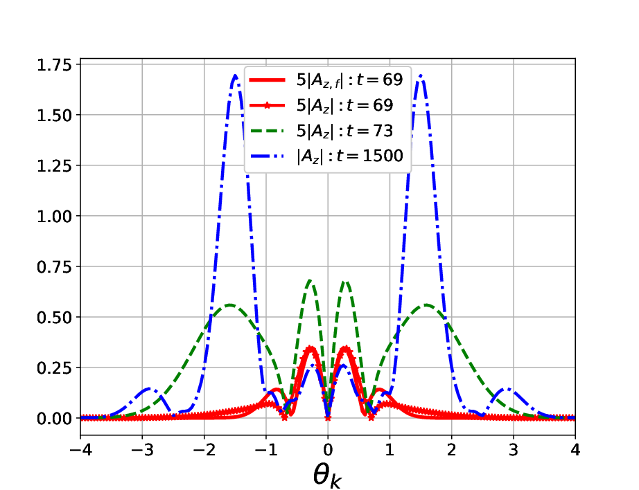
When the ETG grows to the threshold intensity, the spontaneous ZF generation starts and the system evolves to the nonlinear saturation stage. As shown in Fig. (3), ZFs are initially excited around $|\theta_{k}|\gtrsim|\theta_{z,m}|$ in the early nonlinear state ($t=73$). Subsequently, a steady state is gradually reached as ZF spectrum shifts toward $\pm\theta_{z,m}$ and, meanwhile, ETGs are scattered into the linearly stable regime. The effect of long-time-scale ETG-ZF interplay, therefore, is to broaden the ETG radial spectrum, but narrow the ZF spectrum, as vividly illustrated by the snapshots in Fig. (4). The final steady state is characterized by narrow-band ZFs, and the four-wave model is expected to offer a relevant tool for interpreting numerical results of the complicated NLSE model. Figure (5) shows that the time-averaged ZF-ETG ratio, computed from Eqs. (13-14) with $\langle A_{z}^{2}\rangle=A_{z,p}^{2}(\theta_{z}=\theta_{z,m})$ and $\langle A_{n}^{2}\rangle=(1+|\gamma_{n}/\gamma_{s}|)A_{0,p}^{2}(\theta_{z}=\theta_{z,m})$, indeed agrees quantitatively with numerical results. By taking $W\simeq 0.8$ by inspection of Fig. (4), the ZF saturation level $\langle|A_{z}|\rangle=2$ is also in good agreement with the analytical value $|A_{z,p}|\simeq 2.1$. Furthermore, in order to give a qualitative estimate for the corresponding electron heat transport level, one can evaluate the quasilinear electron energy flux lee approximately as $Q_{e}/Q_{gB}\sim\mathcal{O}(|A_{n}|^{2}|k_{\theta}\rho_{e}|)$, where $Q_{gB}=nT_{e}v_{te}\rho_{*}^{2}$ is the gyro-Bohm heat flux. Therefore, for typical plasma conditions, this suggests that the electron heat transport caused by final saturated intermediate-scale toroidal ETG turbulence will be $Q_{e}/Q_{gB}\sim\mathcal{O}(0.1)-\mathcal{O}(1)$, with a linear dependence on the collisionality diamond98.

To summarize, we have derived a nonlinear Schrödinger equation model for the zonal flow generation in ETG turbulence, by allowing plasma non-uniformities and properly taking into account the crucial kinetic effects. It is demonstrated that ZF is easily excited by the intermediate-scale toroidal ETG turbulence, and the corresponding threshold condition is lower than previous fluid predictions by at least $\mathcal{O}(k_{\theta}^{2}\rho_{e}^{2})$, due to the Navier-Stokes type nonlinearity in ETG dynamics. The three-stage evolution of the coherent ETG-ZF system has been addressed. The parallel decoupling effect is found to be essential for determining the narrow-band ZF in the final saturated state. Conversely, the ETG spectrum is broadband since the saturation is achieved via scatterings to the high-$\theta_{k}$ stable regime. Considering typical tokamak parameters, the electron heat transport level expected for the ETG-ZF system is in the range $Q_{e}\lesssim Q_{gB}$ and proportional to the collisionality. Therefore, ZF generation is an efficient nonlinear mechanism for the isotropization and saturation of the intermediate-scale toroidal ETG turbulence. These theoretical findings provide an explanation for the recent gyrokinetic simulation results howard16; colyer; holland17 that show ZF can be important for ETG-driven transport.

Finally, we note that, the present work is readily extended to include the nonlinear toroidal mode coupling of unstable ETGs. For short-wavelength ETG turbulence, the fluid description is applicable, previous studies chen05; lin05 have shown that the toroidal inverse cascade will dominate over the spontaneous ZF excitation, and the resulting turbulence is characterized by streamers. As energy is transferred to intermediate-scale turbulence, however, the ETG-ZF interactions become important and ETG turbulence will be isotropized.

This work is supported by the Exascale Computing Project (17-SC-20-SC), a collaborative effort of the U.S. Department of Energy Office of Science and the National Nuclear Security Administration. We thank Prof. Liu Chen, Dr. Yang Chen and Dr. Junyi Cheng for useful conversations.

References

- (1) S. E. Parker et al., AIP Conf. Proc. 871, 193 (2006).
- (2) N. T. Howard et al., Phys. Plasmas, 23, 056109, (2016).
- (3) G. J. Colyer et al., Plasma Phys. Control. Fusion, 59, 055002, (2017).
- (4) C. Holland, N. T. Howard and B. A. Grierson, Nucl. Fusion 57, 066043 (2017).
- (5) E. J. Kim, C. Holland and P. H. Diamond, Phys. Rev. Lett., 91, 075003, (2003).
- (6) Z. Lin, L. Chen and F. Zonca, Phys. Plasmas, 12, 056125, (2005).
- (7) L. Chen, F. Zonca and Z. Lin, Plasma Phys. Control. Fusion, 47, B71, (2005).
- (8) J. W. Connor, R. J. Hastie and J. B. Taylor, Phys. Rev. Lett., 40, 396, (1978).
- (9) R. A. Frieman and L. Chen, Phys. Fluids, 25, 502, (1982).
- (10) J. Kim and W. Horton, Phys. Fluids B, 3, 1167, (1991)
- (11) M. N. Rosenbluth and F. L. Hinton, Phys. Rev. Lett., 80, 724, (1998).
- (12) P. Ricci, B. N. Rogers and W. Dorland, Phys. Plasmas, 17, 072103, (2010).
- (13) H. Sugama, Phys. Plasmas, 6, 3527, (1999).
- (14) H. T. Chen and L. Chen, Plasma Phys. Control. Fusion, 60, 055011, (2018).
- (15) A. Hasegawa and K. Mima, Phys. Rev. Lett., 39, 205, (2007).
- (16) L. Chen, Z. Lin and R. White, Phys. Plasmas, 7, 3129, (2000).
- (17) Y. C. Lee et al., Phys. Fluids, 30, 1331, (1987).
- (18) P. H. Diamond et al., in Plasma Physics and Controlled Nuclear Fusion Research, 17th IAEA Fusion Energy Conference, Yokohama, Japan, 1998 (International Atomics Energy Agency, Vienna, 1998), p. IAEA-CN-69/TH3/1.