Analysis and approximations of Dirichlet boundary control of Stokes flows in the energy space Thanks: W. Gong was supported in part by the Strategic Priority Research Program of Chinese Academy of Sciences (Grant No. XDB 41000000), the National Key Basic Research Program (Grant No. 2018YFB0704304) and the National Natural Science Foundation of China (Grant No. 11671391 and 12071468). M. Mateos was supported by the Spanish Ministerio de Economía y Competitividad under project MTM2017-83185-P. Y. Zhang are partially supported by the US National Science Foundation (NSF) under grant number DMS-1818867.
Abstract
We study Dirichlet boundary control of Stokes flows in 2D polygonal domains. We consider cost functionals with two different boundary control regularization terms: the norm and an energy space seminorm. We prove well-posedness and regularity results for both problems, develop finite element discretizations for both problems, and prove finite element error estimates for the latter problem. The motivation to study the energy space problem follows from our analysis: we prove that the choice of the control space can lead to an optimal control with discontinuities at the corners, even when the domain is convex. We observe this phenomenon in numerical experiments. This behavior does not occur in Dirichlet boundary control problems for the Poisson equation on convex polygonal domains, and may not be desirable in real applications. For the energy space problem, we derive the first order optimality conditions, and show that the solution of the control problem is more regular than the solution of the problem with the regularization. We also prove a priori error estimates for the control in the energy norm, and present several numerical experiments for both control problems on convex and nonconvex domains.
1 Introduction
PDE-constrained optimal control is an active research area and has been popular for the last several decades. Interest in analysis and computation for problems in this area has been generated by a wide variety of applications and the fast development of computational resources. There are already several monographs and chapters devoted to various aspects of the field, including theoretical analysis, computational methods, and application areas; see, e.g., [34, 46, 6].
Boundary control problems for PDEs are a very important part of this field since for many applications control may only be applied at the boundary of the physical domain. Dirichlet boundary control problems are especially important in application areas, but the problems can be difficult to analyze mathematically – especially when the physical domain has a nonsmooth boundary. One of the key points in the study of Dirichlet boundary control problems is the choice of the control penalty in the cost functional. A natural goal in many applications is to minimize the “amount” of control used, which naturally leads to a boundary control penalty using the norm. This also appears to be a reasonable choice from a numerical approximation point of view. However, in the analysis of such a problem the governing state equation is typically understood in a very weak sense since the Dirichlet boundary condition is only in .
Despite this difficulty, many researchers have considered problems using the control penalty and developed numerical methods and numerical analysis results. One of the first contributions was the study of a finite element method for elliptic Dirichlet boundary control problems in [20]. Control constrained problems governed by semilinear elliptic equations on polygonal domains were studied in [8]. Optimal-order error estimates were derived for the unconstrained problem in [50] for both the control and state by introducing a dual control problem. Higher-order convergence rates were proved in [18] for control-constrained problems in smooth domains based on the superconvergence properties of regular triangulations. In [29] the authors used a mixed finite element method for approximating the elliptic Dirichlet boundary control problem to avoid the very weak formulation of the state equation. For recent results on the regularity of solutions and standard finite element approximations of elliptic Dirichlet boundary control problems we refer to [1], [48] and the references cited therein. In [2], optimal error estimates on general (possibly nonconvex) polygonal domains are obtained for quasi-uniform and superconvergence meshes. Recently, the hybridizable discontinuous Galerkin (HDG) method has applied to the elliptic Dirichlet boundary control problem on convex domains [10, 12, 37, 26, 11]. The HDG method also avoids the very weak formulation, and has a lower computational cost compared to traditional discontinuous Galerkin and mixed methods. We also refer to [24, 27] for error estimates for parabolic Dirichlet boundary control problems, to [49] for state-constrained problems, and to [7] for a Robin penalization approach.
On the other hand, appears to be a natural choice to study the state equation in the standard variational formulation. There are also some numerical analysis results in this direction. The analysis of a finite element method for an elliptic Dirichlet boundary control problem in the energy space setting with as the control space was performed in [54]; a boundary element method for this problem is proposed and analyzed in [53]. In [13] a variation to the energy space method is proposed where the control penalty now involves the harmonic extension of the control into the domain; a posteriori error estimates and the convergence of the adaptive finite element method is studied in [28] for this approach. Also see [40] for another related approach to the energy space method. Sharp convergence rates for the energy space approach have recently been obtained in [58]. There are also other ways to deal with the inhomogeneous Dirichlet boundary condition. In [43, 44, 45] elliptic Dirichlet boundary control problems are studied in the energy space setting using wavelet schemes for the spatial discretization and using a Lagrange multiplier for the inhomogeneous Dirichlet boundary condition.
Dirichlet boundary control problems are of great interest for applications in fluid dynamics; see, for example, [21, 22, 32, 31, 35, 36, 17, 38, 56]. Although many numerical algorithms and simulation results can be found in the literature, there are very few well-posedness, regularity, and numerical analysis results for Dirichlet boundary control problems for fluid flows in polygonal domains.
In this work, we study Dirichlet Stokes flow control problems in 2D polygonal domains using both and for the control spaces. We give precise well-posedness and regularity results for both problems, and show that the regularized optimal control can be discontinuous at the corners of a convex domain. We prove higher regularity for the energy space control problem. We also develop a finite element method for both problems, and prove a prior error estimates for the energy space problem.
Below, we give precise formulations of the Dirichlet Stokes control problems we consider and give a brief overview of related work.
Let be an open bounded domain with polygonal boundary . We let denote the standard Sobolev space with norm and seminorm , and we use bold font to denote vector valued spaces. Set and . We denote the -inner products on , , and by
We use to denote the duality product between and . We let denote the space of traces of for , and we note that for is given by , see [30, Theorem 1.5.2.8]. (This definition does not make sense for .) For , we use to denote the duality product between and .
For the Stokes problem, we use the standard spaces
as well as the velocity spaces (see [57, Section 2.1])
which are Banach spaces with the norm. For , define
and let denote the dual space.
For the control problem, consider a target state , a velocity penalty space , and a control penalty space . Let denote a Tikhonov regularization parameter, and consider the optimal control problem
| (1.1) |
where is the unique solution (either in the transposition sense, see Definition 2.3 below, or standard variational solution) of the Stokes system
| (1.2) | ||||
We note that similar Dirichlet control problems with various choices of the spaces and have been considered in the literature for both the Stokes and Navier-Stokes equations. The choices and were used in the early work [32]. In [17], the spaces and are used for the objective functional; however, the optimal control problem looks for admissible optimal controls in , which is the natural space for the controls to obtain a variational solution of the state equation (1.2). In [38], the authors consider a smooth domain and choose and . We show in polygonal domains that this approach leads to optimal controls that are discontinuous at the corners; see Section 3 for the well-posedness and regularity results. However, a better regularity result for these spaces is obtained if we consider tangential control, i.e., we impose the condition pointwise instead of , see [25] for more details.
Here we focus on the energy space method for the problem in polygonal domains. In Section 4 we formulate the Dirichlet boundary control problem of Stokes equation with velocity space and control space , and we derive the first order optimality condition by using the Steklov-Poincaré operator. Higher regularity of the solutions is shown compared to the setting. In Section 5 we give finite element approximations and error estimates for the energy space method. Numerical experiments are carried out in Section 6 for both choices and in both convex and nonconvex polygonal domains.
Remark 1.1.
Remark 1.2.
The introduction of control constraints does not lead to any differences in the regularity of the solutions or the rates of convergence. Control constrained problems can be treated by means of variational inequalities instead of equalities and there are plenty of examples about this in the literature. We focus on the unconstrained problem in order to avoid additional technicalities.
2 Regularity results
We first summarize the result we presented in [25] about the concept of solution for Dirichlet data in and its precise regularity.
Definitions of very weak solutions of the Stokes and Navier-Stokes equations for data in and even have been given for convex polygonal domains and smooth domains; see [15, Appendix A], [47], [57, Appendix A], and [38, Definition 2.1]. In [25], we showed how to extend the concept to problems posed on nonconvex polygonal domains for data in with some negative , and we also proved that the optimal regularity expected for the solution can be achieved. In [51] a similar result is provided for convex polygonal domains, but only suboptimal regularity for is proved.
To introduce the definition of solution of the state equation, we first need some results about the following compressible Stokes equation:
| (2.1) |
For data , this problem must be understood in the weak sense: Find satisfying
Following [16], we define the singular exponent as the real part of the smallest root different from zero of the equation
| (2.2) |
where denotes the greatest interior angle of . A numerical computation of shows, cf. [16, Figure 2], that , is strictly decreasing, if , and if . Let
| (2.3) |
Theorem 2.1.
[16, Theorem 5.5 (a)] Let satisfy . If and , then Equation 2.1 has a unique solution . Moreover, we have
| (2.4) |
Notice that although the pressure is uniquely determined as a function with the condition , the norm must be taken modulo constant functions. It is important to note that Theorem 2.1 only holds for . This means, even in convex domains one cannot expect in general to have regularity of .
The regularity of can be obtained by requiring an additional condition on the divergence of . For example if with , then the above result holds for (this follows from [16, Theorem 5.5(c)], or the early reference [41] for convex polygonal domains). This implies in a convex domain we have .
This regularity result was used in [15, 51] to define very weak solutions in polygonal domains using as a test function. Although this approach does enable us to define the transposition solution, it does not lead to optimal regularity results for the solution of the Dirichlet control problem.
Later, we also require a regularity result for the case in a convex domain. Let denote the solution of (2.1) for , i.e., and .
Theorem 2.2.
[16, Theorem 5.5(b)(c)] Suppose for some and . If is convex, then the incompressible Stokes equation
| (2.5) |
has a unique solution , , which satisfies
Below, we derive the weak variational form for the state equation (1.2). Since the problem is linear, we may decompose the solution into the contributions from the right hand side and the Dirichlet boundary data . The existence of a unique classical variational solution for is standard and so we may set , see Remark 1.1.
We use interpolation below to give precise regularity results for the state equation (with ), and therefore we define very weak solutions in the case for . Elements of this space do not necessarily satisfy any condition analogous to . In order to account for the constants, we follow [57, Eq. (2.2)] and for with we define the constant
| (2.6) |
This constant satisfies
and we have
This fact, trace theory, and (2.4) give that for we have
| (2.7) |
This allows us to give the following well-defined notion of transposition solution for the state equation (again, with ).
Definition 2.3.
This definition can be formally obtained by integrating by parts twice in the equation and also once in the divergence free condition. We note that this definition can be written in different ways: using two separate equations tested by and (see [38] or [57]), or as one equation (see [15] or [47]).
Furthermore, this definition can be rewritten in different forms when is more regular. First, if , then for every constant and therefore (2.9) can be written as
| (2.10) |
Second, if , then the very weak solution is the variational solution of the problem: Find satisfying
| (2.11) | ||||
Next, we give a regularity result for the state equation (2.8) on polygonal domains from [25, Theorem 2.2]. We note that an analogous result for smooth domains is found in [57, Corollary A.1]. The limiting cases and can be achieved when the domain is smooth; however, this is not possible for polygonal domains.
Theorem 2.4.
If for , then the solution of (2.8) satisfies
Moreover, the control-to-state mapping is continuous from to .
We also recall here the concept of stress force on the boundary as used in [33]. Let be the solution of the incompressible Stokes system with source and Dirichlet data , i.e., and , where is the solution of (2.1) with , and is the solution of (2.11).
For and as above, we define the stress force on the boundary related to to be the unique solution of the variational problem:
| (2.12) |
Notice that for with , integration by parts shows that
| (2.13) |
For , we define by
| (2.14) |
Directly from (2.10) with and (2.13), the adjoint is defined by
| (2.15) |
By Theorem 2.4 we know that is bounded and hence is also bounded. Therefore, is bounded. Specifically, setting gives that for all we have
| (2.16) |
3 Stokes Dirichlet boundary control in
In this section, we investigate the case . For and , our control problem reads
| (3.1) |
where is the solution of the state equation (2.10). By (2.14) we have
| (3.2) | ||||
where and is the tracking term. It is straightforward to prove that
| (3.3) |
Although we are mainly interested in this work in regularization in the energy space , the solution properties of the problem with -regularization are also of interest in order to more clearly see the advantages and disadvantages of energy space control problem. It is also interesting to see the differences between the Dirichlet boundary control of the Poisson equation (cf. [1]) and of the Stokes system.
Using the strict convexity of the functional and the continuity of the control-to-state mapping, which follows from Theorem 2.4, it is standard to prove the existence of a unique solution of problem (). We also prove regularity results below, and show that the optimal control can be discontinuous at the corners of a convex polygonal domain.
Theorem 3.1.
Suppose for some and let be the solution of problem (). Then for all and there exist , , and for all such that , that satisfy the state equation
| (3.4) |
the adjoint state equation
| (3.5) |
and the optimality condition
| (3.6) |
Moreover, there exists such that
and
Finally, if and is convex, then is continuous at a corner if and only if .
Here, the state equation must be understood in the very weak sense (2.10), while the adjoint state equation must be understood in the variational sense.
Proof.
By the definition of in (3.2) and (3.3), the derivative of the objective functional for can be written as
where we used (2.14) and (2.15) in the last equality. The optimality conditions follow in a standard way. For we have that for any . Taking to equal the constant , which is defined in (2.6), we also have that
This implies that is the -projection of onto . Since , we have
The regularity follows from a bootstrapping argument: From Theorem 2.4 we have that . Using this and taking into account that , we have from Theorem 2.2 that , for all such that .
From trace theory, and since , it is clear that
For , and taking , we have that and that . Therefore, (3.6) gives that for all . The regularity of the optimal state follows from Theorem 2.4.
If and is convex, then the gradient of the dual pressure is a function in with . So we have that each component , of , satisfies and on . Therefore, we have that , , for every convex corner (cf. [7, Appendix A]); also, from [7, Lemma A2] and the Sobolev imbedding theorem we have that the normal derivative of is a continuous function. For the pressure, the situation is slightly different. From trace theory we have that and by Sobolev imbeddings we know is a continuous function. Nevertheless, the vector is discontinuous at the corners, and hence the can only be continuous at if . ∎
Remark 3.2.
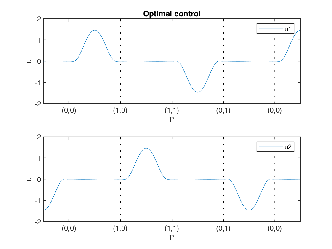
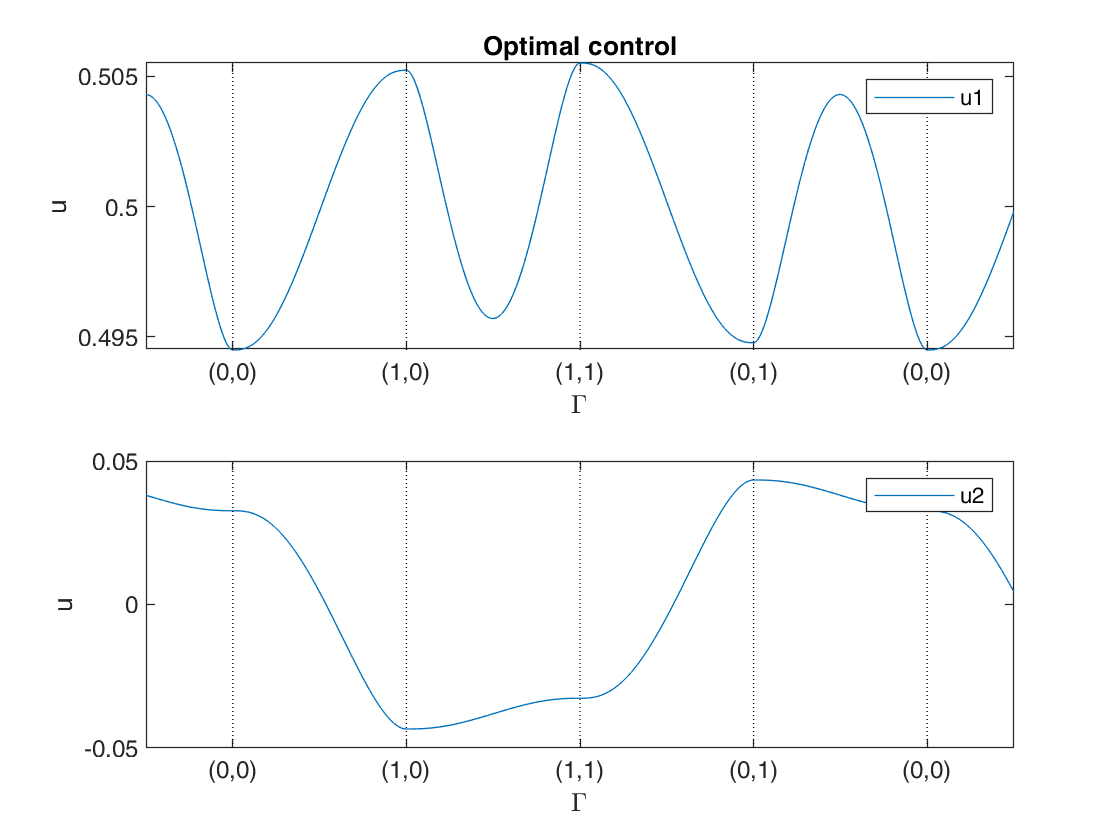
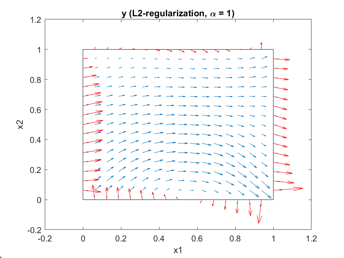
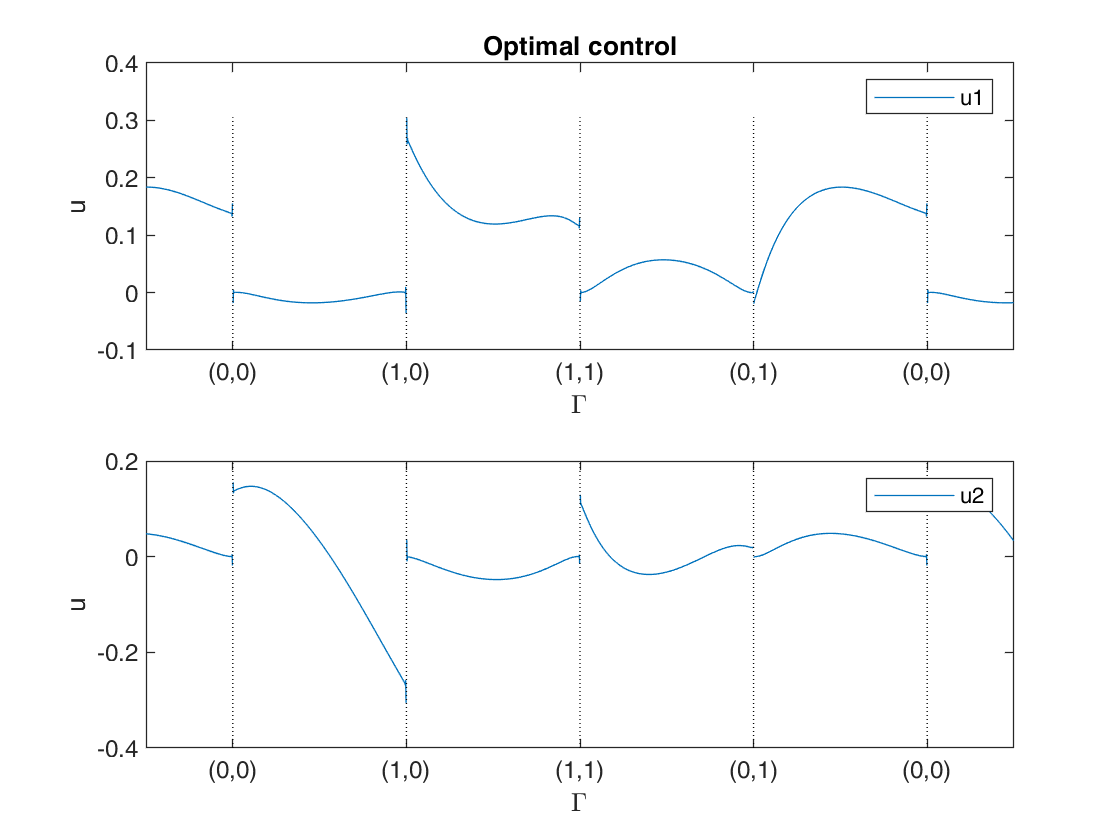
This regularity of the optimal control in a convex domain is essentially different from the regularity achieved by the optimal control of problems related to the Poisson equation. The solution of a problem governed by the Poisson equation must be a continuous function, which is also zero at the corners. In our case, the optimal control may show discontinuities. See Figure 2 for an example with a continuous control and Figure 3 for a problem example with discontinuous control.
Remark 3.3.
Notice that the pressure is determined up to a constant. We choose the pressure such that , but any other representative is of course possible. The value of would change accordingly, so that does not vary.
4 Stokes Dirichlet boundary control in the energy space
Next, we consider Stokes Dirichlet boundary control with a different regularization term:
| (4.1) |
where again we assume and .
There are different kinds of definitions for the -norm, e.g., one may use the Sobolev-Slobodeckii norm or the Fourier transform. The key point to the study of the optimization problem (4.1) is to find an appropriate representation for the -norm that enables us to derive the first order optimality condition. Here we follow the idea of [54] and introduce a Stokes version of the Steklov-Poincaré operator (cf. [3, 19]) associated with (2.10).
It follows from Theorem 2.4 that for any given control , there exists a unique state that satisfies
| (4.2) |
Given , we define by
| (4.3) |
where is any continuous extension operator from to .
Lemma 4.1.
The definition of is independent of the chosen extension and
| (4.4a) | ||||
| (4.4b) | ||||
Proof.
First of all, writing the partial differential equation in divergence form as
gives , and so this function has a well defined normal trace in . It is remarkable too that it is possible to define a variational normal derivative , cf. [7, Lemma A6], and hence is also a well defined element in .
Lemma 4.2.
is a seminorm in equivalent to the seminorm.
Proof.
Let be the projection of onto and set . Notice that and if then . By (4.3) we have
| (4.6) |
and thus we have that is a seminorm in equivalent to the seminorm. ∎
Proceeding similarly to the derivation of (3.2), the precise formulation of our control problem is given by
| (4.7) | ||||
where and
| (4.8) |
The functional being convex and coercive implies that problem (4.7) has a unique solution .
We also note that, by (4.6), an alternative way to write the functional for is
Lemma 4.3.
There exist constants such that for every
and
Proof.
The first property follows immediately from the definition of . Notice that maps into which is continuously embedded in by duality.
Next, we give more insights into the structure of the solution to problem (). The functional in problem (4.7) is Frechét differentiable with respect to . Furthermore, for all , by (4.7) and (4.8) we have
Now we are in the position to derive the regularity of the solution to the minimization problem (4.7).
Theorem 4.4.
Assume for some , and let be the optimal solution of problem (4.7). Then for all and there exist , , and for all such that that satisfy the state equation
the adjoint state equation
and the optimality condition
Moreover, there exists such that
| (4.9) |
Here, both the state equation and the adjoint state equation must be understood in the variational sense.
Proof.
The minimization problem, being a convex problem, is equivalent to the following Euler-Lagrange equation
| (4.10) |
The existence of a unique solution follows immediately from the Lax-Milgram theorem and Lemma 4.3. First order optimality conditions follow in a standard way. Taking , we deduce relation (4.9) as we did for the -regularized problem.
Since , by Theorem 2.4 we have that . From Theorems 2.1 and 2.2, we obtain and for all with . Using the trace theorem (see [30, Theorem 1.5.2.1]) we arrive at
From the trace theorem again on polygons, see [30, Theorem 1.5.2.1] and also [23, Remark 1.1, Chapter 1], we know that there exists some such that on . So we have that and . Using the state equation and the optimality condition (4.9), we deduce that the pair satisfies
This problem has a variational solution, which is unique up to a constant. Noticing that the singular exponents for the Stokes problem with Neumann boundary conditions are the same as those for Dirichlet boundary conditions, see e.g. [55, pp. 191–192], we deduce from Theorem 2.1 that . From the standard trace theorem, we have that . ∎
Remark 4.5.
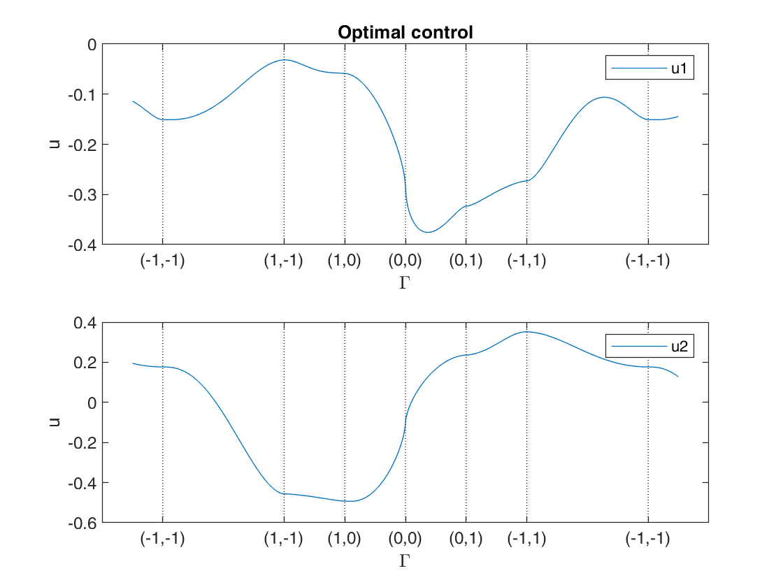
In this case, the optimal control is a continuous function even for problems posed on nonconvex domains; see the second subfigure of Figure 4 in Example 6.3 below.
In order to use the Aubin-Nitsche technique to obtain error estimates in for the control variable, we are also going to study, for any given , the regularity of the unique solution of the problem
A straightforward computation using the definitions of , and , gives
for all . So we have that there exists some such that solves the following Neumann problem
Now we can follow the reasoning of Theorem 4.4. In this case
so we are in the same situation as before, but with , which leads to . Notice that we do not need convexity to obtain this result.
5 FEM for the Stokes Dirichlet energy space control problem
In this section, we consider finite element approximations to the optimal control problem (4.7). We also briefly mention finite element approximations to the problem (3.1) in Remarks 5.4, 5.5, 5.11.
First, we assume that the finite dimensional spaces and satisfy the inf-sup condition: For each there exists a such that
It is well known that the bubble - “Mini” element or the , , “Taylor-Hood” element satisfy the inf-sup condition.
Let , and be the trace of . Let the discrete control space be given by
| (5.1) |
Next, we define the discrete optimization problem:
| (5.2) |
where is a suitable approximation of in the sense that , and the discrete operators and are given below. Here, and in the rest of the paper, is the exponent obtained in Theorem 4.4.
We define the operators and by
| (5.3) |
Here is the finite element approximation of , i.e., satisfies
| (5.4) | ||||
where is the projection of onto . We note for later that satisfies the following standard estimate
| (5.5) |
Next, we give the discrete approximation of the stress force on the boundary, as introduced in [33, Section 3]. For any , we define to be the unique solution of
For and , let and . We define as the approximation of the stress force on the boundary of the pair :
| (5.6) |
Notice that this is exactly the concept of discrete normal derivative; see [8] or, better suited for our purposes, [58]. It is also important to notice that, for , we have that
| (5.7) |
for any linear extension operator . For instance, could be the discrete harmonic extension, the operator , or the zero extension.
For we define as the approximation of the stress force on the boundary of the pair :
| (5.8) |
Lemma 5.1.
is a seminorm in equivalent to the norm.
Proof.
Lemma 5.2.
For every and , we have that
and the adjoint of the restriction of to is given by
| (5.9) |
Proof.
We define as the discrete approximation of the negative stress force on the boundary of the pair :
Consider , notice that and by definition it equals on the boundary. Using the definition of approximate stress force on the boundary, the facts that both and , and also , we obtain
and the proof is complete. ∎
Lemma 5.3.
Problem (5.2) has a unique solution .
Proof.
Following the same notation in Section 4, we define
| (5.10) |
Then the problem (5.2) can be rewritten as:
| (5.11) |
and the unique solution of the discrete problem satisfies the first order optimality condition
| (5.12) |
Remark 5.4.
5.1 Matrix representation of (5.2)
Let and , where are nodal basis functions for ordered so that the first basis functions all vanish on the boundary and the remaining basis functions do not. Then we have . Let , where are nodal basis functions for . For any , , , , we write
We denote , , , , and . Instead of imposing the condition , we choose such that and denote ; see Remark 3.3.
We also let denote the mass matrix representing the standard inner product in , and let denote the stiffness matrix representing the vector Laplace operator on the finite element space . Additionally, denotes the matrix representation of the divergence operator on the involved finite element spaces and . We have
We also use the following submatrices
Since we impose the condition , instead of , we use
Now, we give the implementation details for the discrete optimization problem (5.2). By (5.11), it is equivalent to solve the following equality constrained quadratic programming problem:
| (5.13) |
Let . Define to be the matrix representation of , i.e., for all and , to be the vector representation of , i.e., for all , and to be the vector representation of the constraint, i.e., for all . Then the problem (5.13) can be rewritten as
| (5.14) |
Next, we show how to get the vector representations of and . To do this, we first compute . Consider the discrete extension operator such that on and in the interior nodes of . By the definition of in (5.10) and using (5.9) and (5.7) we have
Now we are in the position to derive the matrix representation of the perturbed Steklov-Poincaré operator . Using (5.8) and (5.7) we have
The problem (5.14) can be easily transformed into an unconstrained problem following the so-called null space method; see e.g. [52, page 462]. We denote and assume, without loss of generality, that . The columns of the null space of form the matrix such that and for . We solve
and then recover . The Lagrange multiplier related to the constraint can also be recovered by means of
We can also write the “big” optimality system. Noticing that
using that and , and taking into account that , we have
where
The above system is not symmetric. There exist alternative symmetric formulations, at the price of the inversion of the stiffness matrix; see e.g. [54, eq. (3.32)] for an antisymmetric version.
Remark 5.5.
To solve the -regularized problem, the procedure is very similar. The only difference, cf. [48], is the computation of , which is done in the following way
where is the mass matrix on the boundary,
An approximation of the quantity can be done using the Lagrange multiplier by means of .
5.2 Error analysis
First, we state the main result in this section.
Theorem 5.6.
Let , with , be the unique solution of problem (4.7) and let be the solution of (5.2). If the conditions in Theorem 4.4 are all fulfilled, then
To prove Theorem 5.6, we assume that the following approximation properties are satisfied (see [23, Chapter II. Section 1.3]):
- (H1)
(Approximation property of ). There exists an operator such that
preserves the boundary conditions, and
- (H2)
(Approximation property of ). There exists an operator such that
These assumptions are satisfied by typical finite element spaces used to solve the Stokes equation, such as the bubble - “Mini” element or the , , “Taylor-Hood” element; see [23, Chap. II, Secs. 4.1 and 4.2], where we take to be the corresponding Lagrange interpolation operator and the projection.
Lemma 5.7.
There exists a constant independent of such that for any and we have
Moreover, if , we have the error estimate
Proof.
The error estimate follows directly from [33, Proposition 17] and Theorems 2.2 and 2.4. ∎
In the next lemma, we collect the approximation properties of , and that will be used to obtain the final error estimate.
Lemma 5.8.
The approximate solution operators , , are bounded, i.e., there exists a constant independent of such that
| (5.15a) | ||||
| (5.15b) | ||||
| (5.15c) | ||||
Moreover, for and , the following error estimates hold:
| (5.16a) | ||||
| (5.16b) | ||||
| (5.16c) | ||||
Proof.
Next, we introduce the following auxiliary problem: find such that
| (5.17) |
where .
Lemma 5.9.
Let , with , be the unique solution of problem (4.7) and be the solution of (5.17). If the conditions in Theorem 4.4 are all fulfilled, then
| (5.18) |
Proof.
First, by (4.10), (5.17), and , we have
| (5.19) |
Next, by Lemma 4.3, we know that is -elliptic and continuous. For any , the error estimate follows in a standard way:
Therefore, there exists such that
The result follows by interpolation (see e.g. [5, Theorem (14.3.3)]), where we take from (H1) and use the regularity of stated in Theorem 4.4.
∎
Now we give the proof of Theorem 5.6.
Proof of Theorem 5.6.
Due to Lemma 5.9, it is enough to obtain the error estimate for .
By the definition of in (5.10) and Lemma 5.1, we know that is coercive on . By the first order conditions satisfied by and in (5.17) and (5.12) and by Young’s inequality, we know that there exists a constant independent of such that
Hence, by the definitions of and in (4.8) and (5.10) we have
For the first term , using the approximation properties of , (4.8), (5.10), (5.16b) and (5.15b), we get
Remark 5.10.
The application of the Aubin-Nitsche technique to the intermediate problem leads easily to
However, using this to obtain error estimates in for is not immediate because satisfies a problem with a perturbed operator and perturbed second member. Following [14, Remark 26.1], the error would be of the same order as
Using the improved error estimate for the discrete approximation of the stress force on the boundary for regular solutions in [33, Proposition 17], we find that the convergence order for those terms can be achieved under the following two assumptions: first, that , which is quite reasonable; but also that is bounded in . But this second assumption requires a higher regularity of the optimal solution; in such a case the order of convergence in would be increased by another .
In numerical experiments, this is the behavior usually observed with the “Mini” finite element: order in and order in .
Remark 5.11.
Although the discretizations of the regularized problem and the regularized problem are very similar, the error analysis performed for the second case cannot be carried out for the first because of the lack of regularity of the solution for , where .
Using the general discretization error estimate of [2, Theorem 3.2], we see that the error is bounded by the best approximation error in the space, the error related to the discretization of the state equation, and the error related to the discrete approximation of the stress force on the boundary. While we have no results for the last two ones, the first one is determined by the Sobolev exponent , so one cannot expect more than for the error.
6 Numerical experiments
In this section we carry out some numerical experiments to compare the solutions of the two control problems (3.1) and (4.7), and also illustrate how the convergence orders can vary due to the shape of the domain and the problem data. We present two examples in a square domain, the first one having a very regular solution, and one example in an L-shaped domain. We discretize each problem using the “Mini” finite element [42] and a family of meshes of size obtained by regular refinement of an initial coarse mesh of size . For one problem, we also discretize using Taylor-Hood elements. Since we do not have the exact solution, we compare the obtained solutions for with the reference solution obtained for , where for the square (a mesh with elements) and for the L-shaped domain (a mesh with elements). For we can solve the “big” optimality system using Matlab’s mldivide. For we run out of memory and solve the reduced optimality system using Matlab’s pcg.
Let , we report the -norm error and the -seminorm error, both computed using the equivalent mesh-independent discrete norms obtained in [9].
Example 6.1.
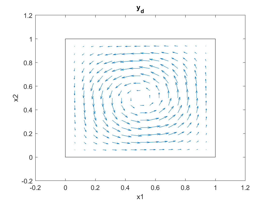
We consider the unit square domain and set the regularization parameter . We choose the forcing , and for the target state we choose the large vortex given in [39],
see the left of Figure 1. For a related example using tangential boundary control, see [25]. The data size in terms of the tracking functional can be measured as . Notice that and on , but it cannot be the solution of the Stokes problem with data since is not a conservative field.
For the regularization, we obtain a value for the tracking term of , while for the regularization we obtain a slightly smaller value . A graph of the state, the optimal control in the energy space, and the solution of the regularized problem can be found in Figure 2. In this case, is a continuous function. Numerically, we find that for all four corners .


The value of the singular exponent for this domain is ; see [16, Table 1]. This means that the exponent giving the order of convergence of the energy regularized problem in the -norm is and the exponent giving the best possible order of convergence of the regularized problem in the norm is . We obtain the results summarized in Table 1 for the optimal control problem with regularization and with regularization. In this case the solution is very regular, the results are similar for both approaches and better than predicted by the general theory. This high regularity can also be noticed in the orders of convergence found for the other variables using higher order Taylor-Hood elements; see Table 2.
| regularization | regularization | ||||||||
| Rate | Rate | Rate | Rate | ||||||
| 4.93E+0 | - | 8.37E-01 | - | 6.17E+0 | - | 9.78E-01 | - | ||
| 1.62E+0 | 1.61 | 2.56E-01 | 1.71 | 2.01E+0 | 1.62 | 3.03E-01 | 1.69 | ||
| 4.82E-01 | 1.75 | 6.80E-02 | 1.91 | 6.37E-01 | 1.65 | 8.00E-02 | 1.92 | ||
| 1.39E-01 | 1.79 | 1.75E-02 | 1.96 | 1.87E-01 | 1.77 | 2.01E-02 | 1.93 | ||
| 4.07E-02 | 1.78 | 4.37E-03 | 2.00 | 5.54E-02 | 1.75 | 5.31E-03 | 1.98 | ||
| Error | Rate | Error | Rate | Error | Rate | ||
| 1.73E-03 | - | 2.36E-02 | - | 2.03E-03 | - | ||
| 2.76E-04 | 2.65 | 8.14E-03 | 1.54 | 3.79E-04 | 2.42 | ||
| 3.69E-05 | 2.90 | 2.20E-03 | 1.89 | 5.13E-05 | 2.89 | ||
| 5.12E-06 | 2.85 | 6.16E-04 | 1.83 | 6.61E-06 | 2.95 | ||
| 7.36E-07 | 2.80 | 1.81E-04 | 1.76 | 1.81E-07 | 2.98 | ||
| 4.54E-04 | - | 9.56E-02 | - | 6.28E-03 | - | ||
| 4.17E-05 | 3.45 | 1.70E-03 | 2.49 | 5.67E-04 | 3.47 | ||
| 4.39E-06 | 3.25 | 3.98E-03 | 2.10 | 4.45E-05 | 3.67 | ||
| 6.50E-07 | 2.75 | 1.26E-04 | 1.65 | 3.75E-06 | 3.57 | ||
| 9.61E-08 | 2.76 | 3.85E-04 | 1.72 | 3.20E-07 | 3.55 | ||
Example 6.2.
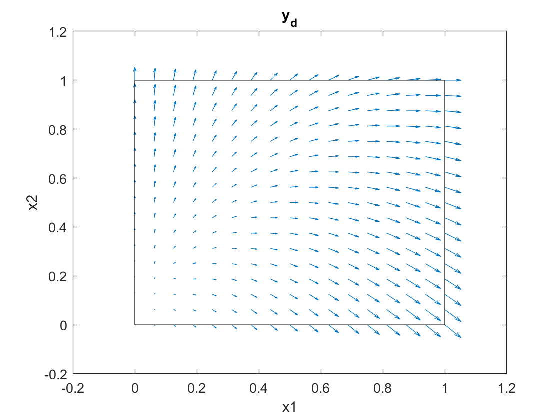
Set , , and . The data size is , and the target does not belong to . A graph of the target field is sketched in the middle of Figure 1.
For the energy regularization, we find ; see the first two subfigures of Figure 3. For the -regularized problem, we have that . The control is discontinuous at the corners, see the last subfigure of Figure 3, and hence is not in . Finite element error results are summarized in Table 3. Again we have and . In this case, the observed experimental order of convergence for the error of the -regularized problem is quite close to .

| regularization | regularization | ||||||
| Rate | Rate | Rate | |||||
| 2.80E-02 | - | 3.77E-03 | - | 1.29E-01 | - | ||
| 9.88E-03 | 1.50 | 1.05E-03 | 1.85 | 8.90E-02 | 0.53 | ||
| 3.34E-03 | 1.57 | 2.81E-04 | 1.90 | 6.22E-02 | 0.52 | ||
| 1.10E-03 | 1.60 | 7.32E-05 | 1.94 | 4.37E-02 | 0.51 | ||
| 3.67E-04 | 1.59 | 1.86E-05 | 1.98 | 3.08E-02 | 0.51 | ||
Example 6.3.
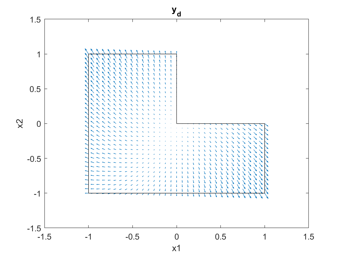
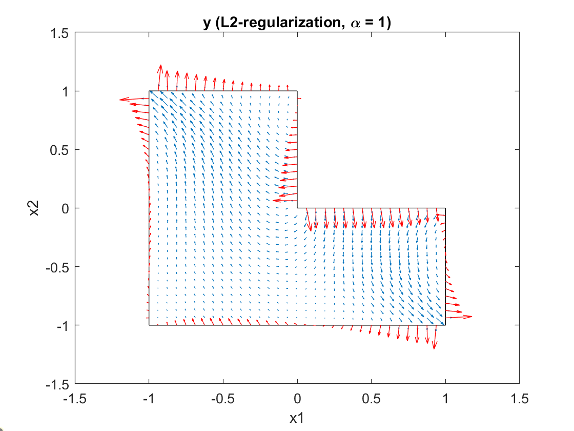
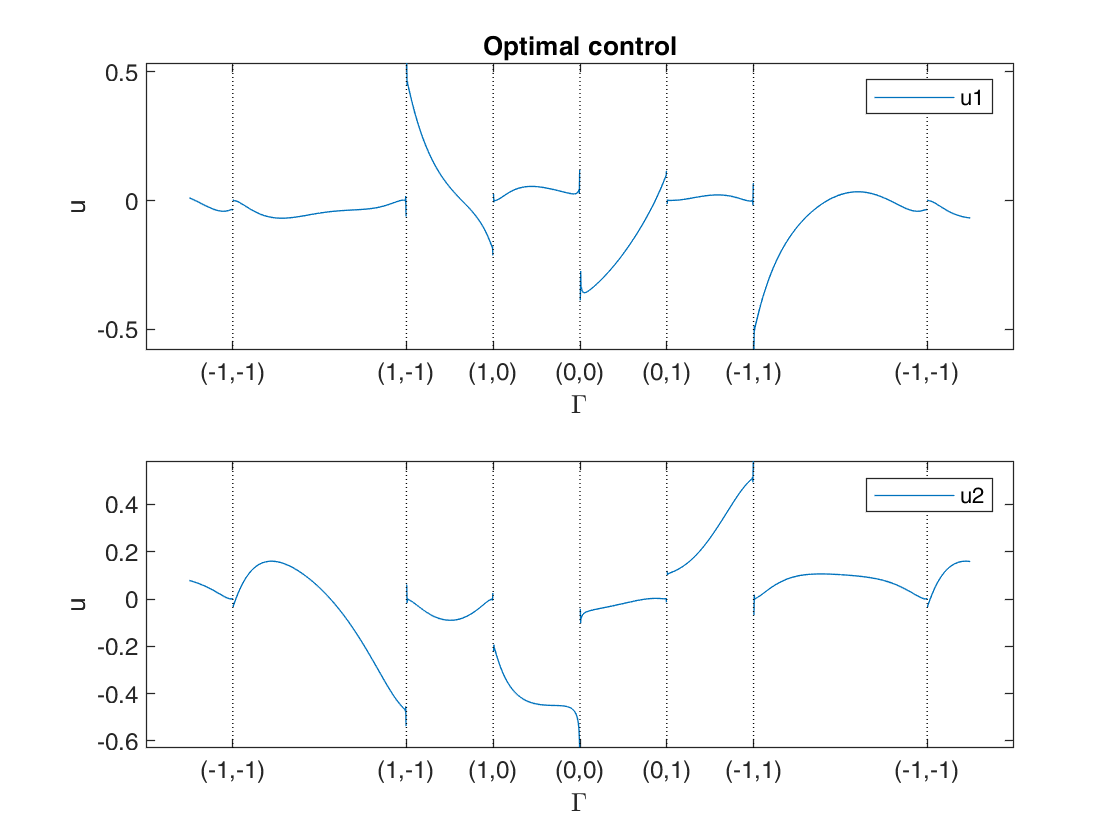
We take the same data as Example 6.2, but now consider the L-shaped domain . The results on this domain are , , . Graphs of the data and the solutions can be found in the right Figure 1 and the first two subfigures of Figure 4. Experimental orders of convergence are in Table 4. The singular exponent for this domain is , so and . The observed orders of convergence are higher.
One remarkable fact is that for the -regularized problem the optimal control need not tend to at a nonconvex corner, as happens with Dirichlet optimal control problems governed by the Poisson equation in a nonconvex polygonal domain.

| regularization | regularization | ||||||
| Rate | Rate | Rate | |||||
| 4.11E-01 | - | 7.40E-02 | - | 3.40E-01 | - | ||
| 2.49E-01 | 0.72 | 3.42E-02 | 1.12 | 2.38E-01 | 0.51 | ||
| 1.53E-01 | 0.71 | 1.55E-02 | 1.14 | 1.71E-01 | 0.48 | ||
| 9.12E-02 | 0.74 | 6.86E-03 | 1.18 | 1.24E-01 | 0.46 | ||
| 5.07E-02 | 0.85 | 2.83E-03 | 1.28 | 8.95E-02 | 0.47 | ||
References
- [1] T. Apel, M. Mateos, J. Pfefferer, and A. Rösch, On the regularity of the solutions of Dirichlet optimal control problems in polygonal domains, SIAM J. Control Optim., 53 (2015), pp. 3620–3641, https://doi.org/10.1137/140994186.
- [2] T. Apel, M. Mateos, J. Pfefferer, and A. Rösch, Error estimates for Dirichlet control problems in polygonal domains: Quasi-uniform meshes, Math. Control Relat. Fields, 8 (2018), pp. 217–245, https://doi.org/10.3934/mcrf.2018010.
- [3] L. Badea, M. Discacciati, and A. Quarteroni, Numerical analysis of the Navier-Stokes/Darcy coupling, Numer. Math., 115 (2010), pp. 195–227, https://doi.org/10.1007/s00211-009-0279-6.
- [4] M. Berggren, Approximations of very weak solutions to boundary-value problems, SIAM J. Numer. Anal., 42 (2004), pp. 860–877, https://doi.org/10.1137/S0036142903382048.
- [5] S. C. Brenner and L. R. Scott, The mathematical theory of finite element methods, vol. 15 of Texts in Applied Mathematics, Springer, New York, third ed., 2008, https://doi.org/10.1007/978-0-387-75934-0.
- [6] E. Casas and M. Mateos, Optimal control of partial differential equations, in Computational mathematics, numerical analysis and applications, vol. 13 of SEMA SIMAI Springer Ser., Springer, Cham, 2017, pp. 3–59.
- [7] E. Casas, M. Mateos, and J.-P. Raymond, Penalization of Dirichlet optimal control problems, ESAIM Control Optim. Calc. Var., 15 (2009), pp. 782–809, https://doi.org/10.1051/cocv:2008049.
- [8] E. Casas and J.-P. Raymond, Error estimates for the numerical approximation of Dirichlet boundary control for semilinear elliptic equations, SIAM J. Control Optim., 45 (2006), pp. 1586–1611, https://doi.org/10.1137/050626600.
- [9] E. Casas and J.-P. Raymond, The stability in spaces of -projections on some convex sets, Numer. Funct. Anal. Optim., 27 (2006), pp. 117–137, https://doi.org/10.1080/01630560600569940.
- [10] G. Chen, G. Fu, J. R. Singler, and Y. Zhang, A Class of Embedded DG Methods for Dirichlet Boundary Control of Convection Diffusion PDEs, J. Sci. Comput., 81 (2019), pp. 623–648, https://doi.org/10.1007/s10915-019-01043-9.
- [11] G. Chen, P. Monk, and Y. Zhang, norm error estimates for hdg methods applied to the poisson equation with an application to the dirichlet boundary control problem, arXiv preprint arXiv:2005.07805, (2020).
- [12] G. Chen, J. R. Singler, and Y. Zhang, An HDG method for Dirichlet boundary control of convection dominated diffusion PDEs, SIAM J. Numer. Anal., 57 (2019), pp. 1919–1946, https://doi.org/10.1137/18M1208708.
- [13] S. Chowdhury, T. Gudi, and A. K. Nandakumaran, Error bounds for a Dirichlet boundary control problem based on energy spaces, Math. Comp., 86 (2017), pp. 1103–1126, https://doi.org/10.1090/mcom/3125.
- [14] P. Ciarlet, Basic error estimates for elliptic problems, in Handbook of Numerical Analysis, P. Ciarlet and J. Lions, eds., vol. II. Finite Element Methods (Part 1), North-Holland, 1991, pp. 17–352.
- [15] C. Conca, Étude d’un fluide traversant une paroi perforée. II. Comportement limite loin de la paroi, J. Math. Pures Appl. (9), 66 (1987), pp. 45–70.
- [16] M. Dauge, Stationary Stokes and Navier-Stokes systems on two- or three-dimensional domains with corners. I. Linearized equations, SIAM J. Math. Anal., 20 (1989), pp. 74–97, https://doi.org/10.1137/0520006.
- [17] J. C. de los Reyes and K. Kunisch, A semi-smooth Newton method for control constrained boundary optimal control of the Navier-Stokes equations, Nonlinear Anal., 62 (2005), pp. 1289–1316, https://doi.org/10.1016/j.na.2005.04.035.
- [18] K. Deckelnick, A. Günther, and M. Hinze, Finite element approximation of Dirichlet boundary control for elliptic PDEs on two- and three-dimensional curved domains, SIAM J. Control Optim., 48 (2009), pp. 2798–2819, https://doi.org/10.1137/080735369.
- [19] M. Discacciati and A. Quarteroni, Analysis of a domain decomposition method for the coupling of Stokes and Darcy equations, in Numerical mathematics and advanced applications, Springer Italia, Milan, 2003, pp. 3–20.
- [20] D. A. French and J. T. King, Approximation of an elliptic control problem by the finite element method, Numer. Funct. Anal. Optim., 12 (1991), pp. 299–314, https://doi.org/10.1080/01630569108816430.
- [21] A. V. Fursikov, M. D. Gunzburger, and L. S. Hou, Boundary value problems and optimal boundary control for the Navier-Stokes system: the two-dimensional case, SIAM J. Control Optim., 36 (1998), pp. 852–894, https://doi.org/10.1137/S0363012994273374.
- [22] A. V. Fursikov, M. D. Gunzburger, and L. S. Hou, Optimal boundary control for the evolutionary Navier-Stokes system: the three-dimensional case, SIAM J. Control Optim., 43 (2005), pp. 2191–2232, https://doi.org/10.1137/S0363012904400805.
- [23] V. Girault and P.-A. Raviart, Finite element methods for Navier-Stokes equations, vol. 5 of Springer Series in Computational Mathematics, Springer-Verlag, Berlin, 1986, https://doi.org/10.1007/978-3-642-61623-5. Theory and algorithms.
- [24] W. Gong, M. Hinze, and Z. Zhou, Finite element method and a priori error estimates for Dirichlet boundary control problems governed by parabolic PDEs, J. Sci. Comput., 66 (2016), pp. 941–967, https://doi.org/10.1007/s10915-015-0051-2.
- [25] W. Gong, W. Hu, M. Mateos, S. J., and Y. Zhang, Analysis of an hybridizable discontinuous Galerkin scheme for the tangential control of the Stokes system, M2AN Math. Model. Numer. Anal., (2020), https://doi.org/10.1051/m2an/2020015,2020.
- [26] W. Gong, W. Hu, M. Mateos, J. Singler, X. Zhang, and Y. Zhang, A New HDG Method for Dirichlet Boundary Control of Convection Diffusion PDEs II: Low Regularity, SIAM J. Numer. Anal., 56 (2018), pp. 2262–2287, https://doi.org/10.1137/17M1152103.
- [27] W. Gong and B. Li, Improved error estimates for semidiscrete finite element solutions of parabolic Dirichlet boundary control problems, IMA Journal of Numerical Analysis, (2019), https://doi.org/10.1093/imanum/drz029.
- [28] W. Gong, W. Liu, Z. Tan, and N. Yan, A convergent adaptive finite element method for elliptic Dirichlet boundary control problems, IMA J. Numer. Anal., 39 (2019), pp. 1985–2015, https://doi.org/10.1093/imanum/dry051.
- [29] W. Gong and N. Yan, Mixed finite element method for Dirichlet boundary control problem governed by elliptic PDEs, SIAM J. Control Optim., 49 (2011), pp. 984–1014, https://doi.org/10.1137/100795632.
- [30] P. Grisvard, Elliptic problems in nonsmooth domains, vol. 24 of Monographs and Studies in Mathematics, Pitman (Advanced Publishing Program), Boston, MA, 1985.
- [31] M. D. Gunzburger, L. Hou, and T. P. Svobodny, Boundary velocity control of incompressible flow with an application to viscous drag reduction, SIAM J. Control Optim., 30 (1992), pp. 167–181, https://doi.org/10.1137/0330011.
- [32] M. D. Gunzburger, L. S. Hou, and T. P. Svobodny, Analysis and finite element approximation of optimal control problems for the stationary Navier-Stokes equations with Dirichlet controls, RAIRO Modél. Math. Anal. Numér., 25 (1991), pp. 711–748, https://doi.org/10.1051/m2an/1991250607111.
- [33] M. D. Gunzburger and S. L. Hou, Treating inhomogeneous essential boundary conditions in finite element methods and the calculation of boundary stresses, SIAM J. Numer. Anal., 29 (1992), pp. 390–424, https://doi.org/10.1137/0729024.
- [34] M. Hinze, R. Pinnau, M. Ulbrich, and S. Ulbrich, Optimization with PDE constraints, vol. 23 of Mathematical Modelling: Theory and Applications, Springer, New York, 2009.
- [35] L. S. Hou and S. S. Ravindran, A penalized Neumann control approach for solving an optimal Dirichlet control problem for the Navier-Stokes equations, SIAM J. Control Optim., 36 (1998), pp. 1795–1814, https://doi.org/10.1137/S0363012996304870.
- [36] L. S. Hou and S. S. Ravindran, Numerical approximation of optimal flow control problems by a penalty method: error estimates and numerical results, SIAM J. Sci. Comput., 20 (1999), pp. 1753–1777, https://doi.org/10.1137/S1064827597325153.
- [37] W. Hu, J. Shen, J. R. Singler, Y. Zhang, and X. Zheng, A superconvergent hybridizable discontinuous Galerkin method for Dirichlet boundary control of elliptic PDEs, Numer. Math., 144 (2020), pp. 375–411, https://doi.org/10.1007/s00211-019-01090-2.
- [38] C. John and D. Wachsmuth, Optimal Dirichlet boundary control of stationary Navier-Stokes equations with state constraint, Numer. Funct. Anal. Optim., 30 (2009), pp. 1309–1338, https://doi.org/10.1080/01630560903499001.
- [39] V. John, A. Linke, C. Merdon, M. Neilan, and L. G. Rebholz, On the divergence constraint in mixed finite element methods for incompressible flows, SIAM Rev., 59 (2017), pp. 492–544, https://doi.org/10.1137/15M1047696.
- [40] M. Karkulik, A Finite Element Method for Elliptic Dirichlet Boundary Control Problems, Comput. Methods Appl. Math., 20 (2020), pp. 827–843, https://doi.org/10.1515/cmam-2019-0104.
- [41] R. B. Kellogg and J. E. Osborn, A regularity result for the Stokes problem in a convex polygon, J. Functional Analysis, 21 (1976), pp. 397–431, https://doi.org/10.1016/0022-1236(76)90035-5.
- [42] J. Koko, KSTOK. MATLAB Central File Exchange., 2020. https://www.mathworks.com/matlabcentral/fileexchange/70996-kstok.
- [43] A. Kunoth, Fast iterative solution of saddle point problems in optimal control based on wavelets, Comput. Optim. Appl., 22 (2002), pp. 225–259, https://doi.org/10.1023/A:1015441724875.
- [44] A. Kunoth, Adaptive wavelet schemes for an elliptic control problem with Dirichlet boundary control, Numer. Algorithms, 39 (2005), pp. 199–220, https://doi.org/10.1007/s11075-004-3630-0.
- [45] A. Kunoth, Optimized wavelet preconditioning, in Multiscale, nonlinear and adaptive approximation, Springer, Berlin, 2009, pp. 325–378, https://doi.org/10.1007/978-3-642-03413-8_10.
- [46] J.-L. Lions, Optimal control of systems governed by partial differential equations, Translated from the French by S. K. Mitter. Die Grundlehren der mathematischen Wissenschaften, Band 170, Springer-Verlag, New York-Berlin, 1971.
- [47] E. Marušić-Paloka, Solvability of the Navier-Stokes system with boundary data, Appl. Math. Optim., 41 (2000), pp. 365–375, https://doi.org/10.1007/s002459911018.
- [48] M. Mateos, Optimization methods for Dirichlet control problems, Optimization, 67 (2018), pp. 585–617, https://doi.org/10.1080/02331934.2018.1426578.
- [49] M. Mateos and I. Neitzel, Dirichlet control of elliptic state constrained problems, Comput. Optim. Appl., 63 (2016), pp. 825–853, https://doi.org/10.1007/s10589-015-9784-y.
- [50] S. May, R. Rannacher, and B. Vexler, Error analysis for a finite element approximation of elliptic Dirichlet boundary control problems, SIAM J. Control Optim., 51 (2013), pp. 2585–2611, https://doi.org/10.1137/080735734.
- [51] M. Moussaoui and A. M. Zine, Existence and regularity results for the Stokes system with non-smooth boundary data in a polygon, Math. Models Methods Appl. Sci., 8 (1998), pp. 1307–1315, https://doi.org/10.1142/S0218202598000603.
- [52] J. Nocedal and S. J. Wright, Numerical optimization, Springer Series in Operations Research, Springer-Verlag, New York, 1999, https://doi.org/10.1007/b98874.
- [53] G. Of, T. X. Phan, and O. Steinbach, Boundary element methods for Dirichlet boundary control problems, Math. Methods Appl. Sci., 33 (2010), pp. 2187–2205, https://doi.org/10.1002/mma.1356.
- [54] G. Of, T. X. Phan, and O. Steinbach, An energy space finite element approach for elliptic Dirichlet boundary control problems, Numer. Math., 129 (2015), pp. 723–748, https://doi.org/10.1007/s00211-014-0653-x.
- [55] M. Orlt and A.-M. Sändig, Regularity of viscous Navier-Stokes flows in nonsmooth domains, in Boundary value problems and integral equations in nonsmooth domains (Luminy, 1993), vol. 167 of Lecture Notes in Pure and Appl. Math., Dekker, New York, 1995, pp. 185–201.
- [56] S. S. Ravindran, Finite element approximation of Dirichlet control using boundary penalty method for unsteady Navier-Stokes equations, ESAIM Math. Model. Numer. Anal., 51 (2017), pp. 825–849, https://doi.org/10.1051/m2an/2016040.
- [57] J.-P. Raymond, Stokes and Navier-Stokes equations with nonhomogeneous boundary conditions, Ann. Inst. H. Poincaré Anal. Non Linéaire, 24 (2007), pp. 921–951, https://doi.org/10.1016/j.anihpc.2006.06.008.
- [58] M. Winkler, Error estimates for variational normal derivatives and Dirichlet control problems with energy regularization, Numer. Math., 144 (2020), pp. 413–445, https://doi.org/10.1007/s00211-019-01091-1.