MS-TP-20-42 Xenon-1T excess as a possible signal of a sub-GeV hidden sector dark matter

Recently the Xenon-1T experiment [1] has analyzed events in the low-energy region of 1–30 keV of electron recoil energy with an exposure of 0.65 tonne-years, while claiming a low background rate of $76\pm 2_{\,\mathrm{stat}}$ events/(tonne-year-keV). The experiment observed an excess of recoil electrons over the background in the 2$-$3 keV range. The collaboration analyzed the axion couplings to electrons, photons and nucleons, and the neutrino magnetic moment as possible sources for the signal. However, these models appear to be in strong tension with stellar constraints [2, 3, 4, 5]. Another possible source of this excess is traces of tritium in xenon of size $(6.2\pm 2.0)\times 10^{-25}$ mol/mol. The experiment currently can neither confirm nor exclude such a possibility. Since the publication of the Xenon-1T results, a variety of models have been proposed which include light sterile neutrinos [6, 7, 8, 9], a goldstino [10], an inflaton [11], string-motivated models [12, 13], boosted dark matter [14, 15, 16], and a variety of other models [17, 18, 19, 20, 21, 22, 23, 24, 25, 26, 27, 28, 29, 30, 31, 32, 33, 34, 35, 36, 37, 38, 39, 40, 41].

In this work we discuss the possibility that the observed effect is a signal from dark matter in the hidden sector. While there are models in the literature where the hidden sector is used for the explanation of the Xenon-1T excess, our analysis differs from them in several ways. In our analysis we use the Stueckelberg extension of the Standard Model where the Stueckelberg sector consists of an additional $U(1)$ gauge boson interacting via kinetic mixing with the visible sector. In many previous works a single Dirac fermion is used which is then split into two Majoranas which are given different masses [32, 30]. In our analysis we consider two Dirac fermions in the hidden sector carrying $U(1)$ charges with a small mass splitting and interacting with the dark photon generated by the Stueckelberg mechanism. In the analysis, both the freeze-in and freeze-out mechanisms operate to generate the desired relic density. The analysis given here satisfies all the relevant constraints on kinetic mixing between the hidden sector and the visible sector and on the dark photon mass from the CRESST 2019 DM-nucleon scattering cross section, from the neutrino experiment CHARM [42] whose results are reinterpreted as limits on the dark photon [43] as well as from the Planck relic density experiment. The outline of the rest of the paper is as follows: In section 2 we discuss the model to explain the Xenon-1T result. In section 3 an analysis of the dark matter relic density is given. A discussion of the inelastic dark matter-electron scattering is given in section 4. Event detection rates in the Xenon-1T detector are discussed in section 5. Constraints on the model and a fit to the Xenon-1T data is given in section 6. Our conclusions are given in section 7. Several details of the calculation are given in the Appendix.

We extend the Standard Model (SM) gauge group by an extra $U(1)_{X}$ under which the SM is neutral. The extra gauge field $C^{\mu}$ mixes with the SM $U(1)_{Y}$ hypercharge $B^{\mu}$ via kinetic mixing [44]. Further, we use the Stueckelberg mechanism [45] to generate mass for the gauge boson of the hidden sector. The total Lagrangian is then given by

$$\mathcal{L}=\mathcal{L}_{\rm SM}+\Delta\mathcal{L},$$

(1)

with

$\displaystyle\Delta\mathcal{L}\supset$

$\displaystyle-\frac{1}{4}C_{\mu\nu}C^{\mu\nu}-\frac{\delta}{2}C_{\mu\nu}B^{\mu\nu}+g_{X}J^{\mu}_{X}C_{\mu}-\frac{1}{2}(\partial_{\mu}\sigma+M_{1}C_{\mu}+M_{2}B_{\mu})^{2},$

(2)

where $g_{X}$ is the gauge coupling in the hidden sector, $J_{X}$ is the hidden sector current and $\sigma$ is a pseudoscalar field which is absorbed in a gauge-invariant way via the Stueckelberg mechanism to give mass to the extra neutral gauge boson which we call $\gamma^{\prime}$ (the dark photon). Further one may introduce matter in the hidden sector which is neutral under $U(1)_{Y}$ but charged under $U(1)_{X}$ [45, 46]. More generally one may have both kinetic mixing and mass mixing [47].

The kinetic energy terms in Eqs. (1) and (2) can be diagonalized by a $GL(2,\mathbb{R})$ transformation

$\displaystyle\left(\begin{matrix}C^{\mu}\cr B^{\mu}\end{matrix}\right)=\left(\begin{matrix}c_{\delta}&0\cr-s_{\delta}&1\end{matrix}\right)\left(\begin{matrix}C^{\prime\mu}\cr B^{\prime\mu}\end{matrix}\right),$

(3)

where $c_{\delta}=1/(1-\delta^{2})^{1/2}$ and $s_{\delta}=\delta/(1-\delta^{2})^{1/2}$.

In the Standard Model the neutral gauge boson sector arises from the hypercharge gauge boson $B^{\mu}$ and the third component of the $SU(2)_{L}$ gauge field $A^{\mu}_{a}$ ($a=$ 1$-$3), which leads to a $2\times 2$ mass squared matrix after spontaneous symmetry breaking. It contains one massless mode, the photon, and a massive mode, the $Z$-boson. Inclusion of the Stueckelberg gauge field $C_{\mu}$ enlarges the $2\times 2$ mass squared matrix of the neutral gauge boson sector in the standard model to a $3\times 3$ mass squared matrix in the Stueckelberg extended model. Thus after spontaneous electroweak symmetry breaking and the Stueckelberg mass growth, and on including the $GL(2,\mathbb{R})$ transformation to obtain a diagonal and a normalized kinetic energy for the gauge bosons, the $3\times 3$ mass squared matrix of neutral vector bosons in the basis $(C^{\prime}_{\mu},B^{\prime}_{\mu},A^{3}_{\mu})$ is given by

$\displaystyle\mathcal{M}^{2}_{V}=\left(\begin{matrix}M_{1}^{2}\kappa^{2}+\frac{1}{4}g^{2}_{Y}v_{H}^{2}s^{2}_{\delta}&\kappa\epsilon M_{1}^{2}-\frac{1}{4}g^{2}_{Y}v_{H}^{2}s_{\delta}&\frac{1}{4}g_{Y}g_{2}v_{H}^{2}s_{\delta}\cr\kappa\epsilon M_{1}^{2}-\frac{1}{4}g^{2}_{Y}v_{H}^{2}s_{\delta}&\epsilon^{2}M_{1}^{2}+\frac{1}{4}g^{2}_{Y}v_{H}^{2}&-\frac{1}{4}g_{Y}g_{2}v_{H}^{2}\cr\frac{1}{4}g_{Y}g_{2}v_{H}^{2}s_{\delta}&-\frac{1}{4}g_{Y}g_{2}v_{H}^{2}&\frac{1}{4}g^{2}_{2}v_{H}^{2}\cr\end{matrix}\right),$

(4)

where $g_{2}$ is the $SU(2)_{L}$ gauge coupling, $\kappa=(c_{\delta}-\epsilon s_{\delta})$, $\epsilon=M_{2}/M_{1}$ and $v_{H}$ is the Higgs VEV. The mass-squared matrix of Eq. (4) has one zero eigenvalue which is the photon, while the other two eigenvalues are

$$M^{2}_{\pm}=\frac{1}{2}\left\{M^{2}_{0}\pm\sqrt{M_{0}^{4}-M_{1}^{2}v_{H}^{2}\Big[(\kappa^{2}+\epsilon^{2})g_{2}^{2}+g^{2}_{Y}c^{2}_{\delta}\Big]}~\right\},$$

(5)

where $M^{2}_{0}=(\kappa^{2}+\epsilon^{2})M_{1}^{2}+\dfrac{1}{4}v_{H}^{2}(g_{Y}^{2}c^{2}_{\delta}+g_{2}^{2})$. Here $M_{-}$ is identified as the $\gamma^{\prime}$ boson mass, while $M_{+}$ as the $Z$ boson. The diagonalization of the mass-squared matrix of Eq. (4) can be done via two orthogonal transformations, where the first is given by [47]

$\displaystyle\mathcal{O}=\left(\begin{matrix}1/c_{\delta}&-s_{\delta}/c_{\delta}&0\cr s_{\delta}/c_{\delta}&1/c_{\delta}&0\cr 0&0&1\cr\end{matrix}\right),$

(6)

which transforms the mass matrix to $\mathcal{M^{\prime}}^{2}_{V}=\mathcal{O}^{T}\mathcal{M}^{2}_{V}\mathcal{O}$,

$\displaystyle\mathcal{M^{\prime}}^{2}_{V}=\left(\begin{matrix}M_{1}^{2}&M_{1}^{2}\bar{\epsilon}&0\cr M_{1}^{2}\bar{\epsilon}&M_{1}^{2}\bar{\epsilon}^{2}+\frac{1}{4}g^{2}_{Y}v_{H}^{2}c^{2}_{\delta}&-\frac{1}{4}g_{Y}g_{2}v_{H}^{2}c_{\delta}\cr 0&-\frac{1}{4}g_{Y}g_{2}v_{H}^{2}c_{\delta}&\frac{1}{4}g^{2}_{2}v_{H}^{2}\cr\end{matrix}\right),$

(7)

where $\bar{\epsilon}=\epsilon c_{\delta}-s_{\delta}$. The gauge eigenstates of $\mathcal{M^{\prime}}^{2}_{V}$ can be rotated into the corresponding mass eigenstates $(\gamma^{\prime},Z,\gamma)$ using the second transformation such that $\mathcal{R}^{T}\mathcal{M^{\prime}}^{2}_{V}\mathcal{R}=\text{diag}(m^{2}_{\gamma^{\prime}},m^{2}_{Z},0)$ where the rotation matrix is given by

$\displaystyle\mathcal{R}=\left(\begin{matrix}\cos\psi\cos\phi-\sin\theta\sin\phi\sin\psi&\sin\psi\cos\phi+\sin\theta\sin\phi\cos\psi&-\cos\theta\sin\phi\cr\cos\psi\sin\phi+\sin\theta\cos\phi\sin\psi&\sin\psi\sin\phi-\sin\theta\cos\phi\cos\psi&\cos\theta\cos\phi\cr-\cos\theta\sin\psi&\cos\theta\cos\psi&\sin\theta\cr\end{matrix}\right).$

(8)

Here the mixing angles are given by

$$\tan\phi=\bar{\epsilon},~~~\tan\theta=\frac{g_{Y}}{g_{2}}c_{\delta}\cos\phi,$$

(9)

and

$$\tan 2\psi\simeq\frac{2\bar{\epsilon}m^{2}_{Z}\sin\theta}{m^{2}_{\gamma^{\prime}}-m^{2}_{Z}+(m^{2}_{\gamma^{\prime}}+m^{2}_{Z}-m^{2}_{W})\bar{\epsilon}^{2}},$$

(10)

where $m_{W}=g_{2}v_{H}/2$, $m_{\gamma^{\prime}}\equiv M_{-}$ and $m_{Z}\equiv M_{+}$. Since the dark photon mixes with the SM gauge bosons, it will couple with the SM fermions and so

$$\mathcal{L}_{\rm SM}=\frac{g_{2}}{2\cos\theta}\bar{\psi}_{f}\gamma^{\mu}\Big[(v_{f}-\gamma_{5}a_{f})Z_{\mu}+(v^{\prime}_{f}-\gamma_{5}a^{\prime}_{f})A^{\gamma^{\prime}}_{\mu}\Big]\psi_{f}+e\bar{\psi}_{f}\gamma^{\mu}Q_{f}A_{\mu}\psi_{f},$$

(11)

where $f$ runs over all SM fermions and the vector and axial couplings are given by

	$\displaystyle v_{f}$	$\displaystyle=\cos\psi[(1-\bar{\epsilon}\tan\psi\sin\theta)T_{3f}-2\sin^{2}\theta(1-\bar{\epsilon}\csc\theta\tan\psi)Q_{f}],$		(12)
	$\displaystyle a_{f}$	$\displaystyle=\cos\psi(1-\bar{\epsilon}\tan\psi\sin\theta)T_{3f},$
	$\displaystyle v^{\prime}_{f}$	$\displaystyle=-\cos\psi[(\tan\psi+\bar{\epsilon}\sin\theta)T_{3f}-2\sin^{2}\theta(\bar{\epsilon}\csc\theta+\tan\psi)Q_{f}],$
	$\displaystyle a^{\prime}_{f}$	$\displaystyle=-\cos\psi(\tan\psi+\bar{\epsilon}\sin\theta)T_{3f}.$

Here $T_{3f}$ is the third component of the isospin and $Q_{f}$ is the electric charge.

We assume that the hidden sector where $C^{\mu}$ resides contains two mass degenerate Dirac fermions $D_{1}$ and $D_{2}$ with the common mass $\mu$ which, however, carry different charges $Q_{1}$ and $Q_{2}$ under the $U(1)_{X}$ gauge group. The interaction Lagrangian for the hidden sector is then given by

$\displaystyle\mathcal{L}^{\rm int}_{D}=$

$\displaystyle-g^{\gamma^{\prime}}_{X}Q_{1}\bar{D}_{1}\gamma^{\mu}D_{1}A_{\mu}^{\gamma^{\prime}}-g^{\gamma^{\prime}}_{X}Q_{2}\bar{D}_{2}\gamma^{\mu}D_{2}A_{\mu}^{\gamma^{\prime}}-g^{Z}_{X}Q_{1}\bar{D}_{1}\gamma^{\mu}D_{1}Z_{\mu}-g^{Z}_{X}Q_{2}\bar{D}_{2}\gamma^{\mu}D_{2}Z_{\mu},$

(13)

with $g^{\gamma^{\prime}}_{X}=g_{X}(\mathcal{R}_{11}-s_{\delta}\mathcal{R}_{21})$ and $g^{Z}_{X}=g_{X}(\mathcal{R}_{12}-s_{\delta}\mathcal{R}_{22})$, where $\mathcal{R}_{ij}$ are elements of the matrix in Eq. (8). To generate inelastic scattering we need to split the masses of the $D$-fermions. To this end we add a $U(1)_{X}$ gauge violating mass terms $\Delta\mu(\bar{D}_{1}D_{2}+\text{h.c.})$ so that the Lagrangian for the $(D_{1},D_{2})$ mass terms is given by

$\displaystyle\mathcal{L}^{\rm mass}_{D}=-\mu(\bar{D}_{1}D_{1}+\bar{D}_{2}D_{2})-\Delta\mu(\bar{D}_{1}D_{2}+\bar{D}_{2}D_{1}),$

(14)

We can now go to the mass diagonal basis with Dirac fermions $D_{1}^{\prime}$ with mass $m_{1}=\mu-\Delta\mu$ and $D_{2}^{\prime}$ with mass $m_{2}=\mu+\Delta\mu$ and we assume $m_{2}>m_{1}$ so $D_{2}^{\prime}$ is the heavier of the two dark fermions. In this basis, Eq. (13) takes the form

	$\displaystyle-\mathcal{L}^{\rm int}_{D}$	$\displaystyle=\frac{1}{2}g^{\gamma^{\prime}}_{X}(Q_{1}+Q_{2})\left(\bar{D}_{1}^{\prime}\gamma^{\mu}D_{1}^{\prime}+\bar{D}_{2}^{\prime}\gamma^{\mu}D_{2}^{\prime}\right)A_{\mu}^{\gamma^{\prime}}$		(15)
		$\displaystyle+\frac{1}{2}g^{\gamma^{\prime}}_{X}(Q_{1}-Q_{2})(\bar{D}_{1}^{\prime}\gamma^{\mu}D_{2}^{\prime}+\bar{D}_{2}^{\prime}\gamma^{\mu}D_{1}^{\prime})A_{\mu}^{\gamma^{\prime}}$
		$\displaystyle+\frac{1}{2}g^{Z}_{X}(Q_{1}+Q_{2})\left(\bar{D}_{1}^{\prime}\gamma^{\mu}D_{1}^{\prime}+\bar{D}_{2}^{\prime}\gamma^{\mu}D_{2}^{\prime}\right)Z_{\mu}$
		$\displaystyle+\frac{1}{2}g^{Z}_{X}(Q_{1}-Q_{2})(\bar{D}_{1}^{\prime}\gamma^{\mu}D_{2}^{\prime}+\bar{D}_{2}^{\prime}\gamma^{\mu}D_{1}^{\prime})Z_{\mu}.$

From Eq. (11) and Eq. (15) we note that the dark photon has couplings with both the visible sector and the hidden sector. Thus from Eq. (11) we find that the dark photon couples with quarks and leptons in the visible sector while from Eq. (15) we find that the dark photon has couplings with $D_{1}^{\prime},D_{2}^{\prime}$ in the dark sector. These couplings allow for an inelastic scattering process to occur where a dark fermion hits a bound electron in a xenon atom producing, in an exothermic process, a recoil electron with excess energy, i.e.,

$\displaystyle e+D_{2}^{\prime}\to e^{\prime}+D_{1}^{\prime},$

(16)

where the final electron receives an extra boost in energy from the mass difference $\Delta m=m_{2}-m_{1}=2\Delta\mu$.

Since the hidden sector matter has feeble couplings with the Standard Model particles, they are never in thermal equilibrium with the visible sector and the usual freeze-out analysis for the computation of the relic density does not apply. However, the hidden sector particles can be produced via the annihilation of the Standard Model particles into dark photons and dark fermions via these feeble interactions and the computation of the relic density in this case is computed using the freeze-in mechanism [48]. Within the dark sector itself the dark fermions and the dark photons interact via normal size interactions and are in thermal equilibrium up to a certain freeze-out temperature $T_{f}$ via the process $D\bar{D}\to\gamma^{\prime}\gamma^{\prime}$. However, below the dark sector freeze-out temperature $T_{f}$, the dark fermions and the dark photons decouple and the dark photons decay to the visible sector much before the big bang nucleosynthesis, which leaves the dark fermions as the only DM candidates. In our model we assume that the visible and hidden sectors have the same temperature. One can consider sectors with different temperatures in the early universe, but it has been shown that the two sectors will eventually thermalize and that the effect on the relic density is minimal [49].

For calculating the DM relic density of $D^{\prime}_{1}$ and $D^{\prime}_{2}$, we assume $m_{1}\simeq m_{2}\simeq m_{D}$ and write only one Boltzmann equation for the dark fermion. In this limit, we have

$$\frac{dY_{D}}{dx}\approx-1.32M_{\rm Pl}\frac{h_{\rm eff}(T)}{g^{1/2}_{\rm eff}(T)}\frac{m_{D}}{x^{2}}\left(-\langle\sigma v\rangle_{D\bar{D}\to i\bar{i}}Y_{D}^{\rm eq^{2}}+\langle\sigma v\rangle_{D\bar{D}\to\gamma^{\prime}\gamma^{\prime}}Y^{2}_{D}\right),$$

(17)

where $Y_{D}=n/s$ is the comoving number density (or yield) of DM, $h_{\rm eff}$ and $g_{\rm eff}$ are the entropy and energy density numbers of degrees of freedom, $M_{\rm Pl}$ is the reduced Planck mass ($M_{\rm Pl}\sim 2.4\times 10^{16}$ GeV) and $x=m_{D}/T$. The first term on the right-hand-side of Eq. (17) is the production of dark matter particles via the freeze-in mechanism and the second term produces DM depletion. Here the thermally averaged cross-section is given by

$$\langle\sigma v\rangle^{D\bar{D}\to ab}(x)=\frac{x}{8m^{5}_{D}K^{2}_{2}(x)}\int_{4m_{D}^{2}}^{\infty}ds~\sigma(s)\sqrt{s}\,(s-4m_{D}^{2})K_{1}\left(\frac{\sqrt{s}}{m_{D}}x\right),$$

(18)

while the equilibrium yield is given by

$$Y_{D}^{\rm eq}(x)=\frac{45}{4\pi^{4}}\frac{g_{D}}{h_{\rm eff}(T)}x^{2}K_{2}(x).$$

(19)

Here $g_{D}$ is the dark fermion number of degrees of freedom, $K_{1}$ and $K_{2}$ are the modified second order Bessel functions of degree one and two. The Boltzmann equation Eq. (17) is solved numerically to determine the yield at the present time $Y_{\infty}$ which gives us the relic density

$$\Omega h^{2}=\frac{m_{D}Y_{\infty}s_{0}h^{2}}{\rho_{c}},$$

(20)

where $s_{0}$ is today’s entropy density, $\rho_{c}$ is the critical density and $h=0.678$ denotes the present Hubble expansion rate in units of 100 km s^-1 Mpc^-1.

We select three benchmarks with different masses for the dark photon and for the dark fermions. The benchmarks are listed in Table 1 along with the couplings, the relic density and the inelastic DM-electron scattering cross-section. In the analysis, we set $\epsilon=0$, i.e. we assume no mass mixing.

The DM relic density satisfies, within theoretical uncertainties, the experimental value from the Planck Collaboration [50]

$$(\Omega h^{2})_{\rm Planck}=0.1198\pm 0.0012.$$

(21)

Following the dark freeze-out of DM in the hidden sector, conversion processes $D^{\prime}_{2}\bar{D}^{\prime}_{2}\longleftrightarrow D^{\prime}_{1}\bar{D}^{\prime}_{1}$ remain active. The ratio of the number densities of $D^{\prime}_{1}$ and $D^{\prime}_{2}$ is Boltzmann suppressed, i.e., $n_{2}/n_{1}\sim\exp(-\Delta m/T_{c})$, where $T_{c}$ is the temperature below which conversion processes shut off. One can safely assume that $n_{2}\sim n_{1}$ as long as $T_{c}\gg\Delta m$. Focusing on the process $D^{\prime}_{2}\bar{D}^{\prime}_{2}\longrightarrow D^{\prime}_{1}\bar{D}^{\prime}_{1}$, we determine $T_{c}$ for which

$$n_{2}\langle\sigma v\rangle_{D^{\prime}_{2}\bar{D}^{\prime}_{2}\longrightarrow D^{\prime}_{1}\bar{D}^{\prime}_{1}}/H\sim 1,$$

(22)

where $H$ is the Hubble parameter. In Fig. 1 we plot $n\langle\sigma v\rangle$ versus $x$ for benchmarks (a) (left panel) and (c) (right panel). The figure shows the conversion process (blue) along with two other processes, $D\bar{D}\to i\bar{i}$ (red) and $D\bar{D}\to\gamma^{\prime}\gamma^{\prime}$ (yellow) and the Hubble parameter (purple). For benchmark (a), one finds that for the value of the kinetic mixing chosen the DM remains out of equilibrium with the SM for the entire $x$ range, while increasing the kinetic mixing causes such a process to enter in equilibrium for a range of $x$ as shown for benchmark (c). This process, however, decouples before other decoupling processes.

As also shown in Fig. 1, dark freeze-out occurs for $x\sim 20$ for all benchmarks. Turning to the conversion process, for benchmark (a), such a process shuts off at $x\sim 1.12\times 10^{4}$, which for the DM mass of benchmark (a) corresponds to $T_{c}\sim 90$ keV. The mass gap of interest here is $\Delta m\sim 2.8$ keV which makes the number densities of $D^{\prime}_{1}$ and $D^{\prime}_{2}$ almost equal. One can see that the conversion process shuts off much later than the other ones. This is also observed for benchmark (b). Unlike (a) and (b), benchmark (c) shows the freeze-out and conversion process shutting off occur at the same $x\sim 20$ which corresponds to a temperature much larger than $\Delta m$. Thus for practical purposes hereafter, we assume that the DM density is divided equally between $D^{\prime}_{1}$ and $D^{\prime}_{2}$.

After the conversion process terminates, the dark fermion $D_{2}^{\prime}$ can decay to $D_{1}^{\prime}$. The only decay channel would be $D_{2}^{\prime}\to D_{1}^{\prime}\bar{\nu}\nu$, which is further suppressed by the dark photon coupling to the neutrinos which is proportional to the kinetic mixing, and further the decay is phase-space suppressed because of the small mass gap $\Delta m\sim\mathcal{O}$(keV). The total 3-body decay width is (including three neutrino generations)

$$\Gamma_{D_{2}^{\prime}\to D_{1}^{\prime}\nu\bar{\nu}}=\frac{x_{\nu}^{2}}{256\pi^{3}m^{4}_{\gamma^{\prime}}}\left[\frac{f(m_{1},m_{2})}{m_{2}^{3}}+24m_{1}^{3}(m_{1}^{2}+m_{1}m_{2}+m^{2}_{2})\log\left(\frac{m_{2}}{m_{1}}\right)\right],$$

(23)

where

$$f(m_{1},m_{2})=(m_{2}^{2}-m_{1}^{2})(m_{1}^{6}-2m_{2}m_{1}^{5}-7m_{2}^{2}m_{1}^{4}-20m_{2}^{3}m_{1}^{3}-7m_{2}^{4}m_{1}^{2}-2m_{2}^{5}m_{1}+m_{2}^{6}).$$

(24)

Since $m_{1}=m_{2}-\Delta m$ and expanding in $\Delta m$, we get to lowest order in $\Delta m$

$$\Gamma_{D_{2}^{\prime}\to D_{1}^{\prime}\nu\bar{\nu}}\simeq\frac{x_{\nu}^{2}(\Delta m)^{5}}{40\pi^{3}m^{4}_{\gamma^{\prime}}},$$

(25)

where for a small gauge kinetic mixing, $g_{X}^{\gamma^{\prime}}\approx g_{X}$ and

$$x_{\nu}\sim g_{X}g_{Y}(Q_{1}-Q_{2})\left(\frac{m_{\gamma^{\prime}}}{m_{Z}}\right)\delta.$$

(26)

In this work we are interested in $\Delta m\sim 3$ keV and $\delta\sim 10^{-5}$ which results in a decay lifetime of $D_{2}^{\prime}$ order $10^{13}$ years which means that $D_{2}^{\prime}$ is stable over the lifetime of the universe. Thus, in this model dark matter is constituted of two dark fermions with essentially degenerate masses which are of order 1 GeV.

A DM particle can undergo an elastic scattering with a bound electron in a xenon atom, but such a scattering can deliver only a few eV to the electron which is not sufficient to explain the Xenon-1T excess. However, an inelastic exothermic down-scattering can impart a recoil energy to the electron equivalent to the mass difference between the incoming and outgoing DM particles. The model considered here allows for the desired small mass splitting between the two Dirac fermions $D^{\prime}_{1}$ and $D^{\prime}_{2}$ so that the heavier fermion $D^{\prime}_{2}$ down-scatters to $D^{\prime}_{1}$. Next, we compute the inelastic scattering cross-section of the process described $D_{2}^{\prime}(\vec{p}_{1})+e(\vec{p}_{2})\to D_{1}^{\prime}(\vec{p}_{3})+e^{\prime}(\vec{p}_{4})$. Assuming the dark photon mass is much greater than the momentum transfer, the averaged matrix element squared for this process is given by

	$\displaystyle\overline{|\mathcal{M}|^{2}}$	$\displaystyle=\frac{2\bar{g}_{X}^{2}g_{2}^{2}}{m^{4}_{\gamma^{\prime}}\cos^{2}\theta}\Bigg\{\frac{1}{2}(a_{f}^{\prime 2}-v_{f}^{\prime 2})\Big[(m_{1}-m_{2})^{2}-(t+2m_{1}m_{2})\Big]m^{2}_{e}+\frac{1}{4}(v_{f}^{\prime 2}+a_{f}^{\prime 2})\Big[(m_{2}^{2}+m_{e}^{2}-u)$
		$\displaystyle\times(m_{1}^{2}+m_{e}^{2}-u)+(s-m_{1}^{2}-m_{e}^{2})(s-m_{2}^{2}-m_{e}^{2})-2m_{1}m_{2}(2m_{e}^{2}-t)\Big]\Bigg\},$		(27)

where $\bar{g}_{X}=\frac{1}{2}g_{X}(Q_{1}-Q_{2})$ and $s,t,u$ are the Mandelstam variables. The directional matrix element for free electron-DM scattering is given by

$$\overline{|\mathcal{M}(\vec{q})|^{2}}=\overline{|\mathcal{M}(q)|^{2}}\times|F_{DM}(q)|^{2},$$

(28)

where the form factor $F_{DM}(q)$ can be taken as 1 for a small momentum transfer. The electron-DM scattering differential cross-section is given by

$\displaystyle\frac{d\bar{\sigma}_{e}}{d\Omega}$

$\displaystyle=\frac{1}{64\pi^{2}s}\frac{|\vec{p}_{3}|}{|\vec{p}_{1}|}\overline{|\mathcal{M}(\vec{q})|^{2}}.$

(29)

Keeping the velocity dependence in the Mandelstam variables, we have

$$t=-q^{2}\simeq-\Delta m\left(1-\sqrt{\frac{2m_{e}v^{2}}{\Delta m}}\cos\theta_{\rm CM}\right),~~~s\sim(m_{2}+m_{e})^{2}\left(1+\frac{\mu_{De}}{m_{2}+m_{e}}v^{2}\right),$$

(30)

and integrating over $\theta_{\rm CM}$, the scattering angle in the CM frame, and $\phi$, we get for the DM-e scattering cross-section

$$\bar{\sigma}_{e}\simeq\frac{\bar{g}_{X}^{2}g_{2}^{2}}{16\pi m^{4}_{\gamma^{\prime}}\cos^{2}\theta}\left(\frac{4\mu^{2}_{De}}{1+\frac{\mu_{De}}{m_{2}+m_{e}}v^{2}}\right)\left[v^{\prime 2}_{f}+(a_{f}^{\prime 2}+v^{\prime 2}_{f})v^{2}\right],$$

(31)

where $\mu_{De}=\frac{m_{2}m_{e}}{m_{2}+m_{e}}$ is the dark matter-electron reduced mass. For $v\sim 10^{-3}$, one can discard the velocity-dependent piece and get

$$\bar{\sigma}_{e}\simeq\frac{\bar{g}_{X}^{2}g_{2}^{2}}{4\pi\cos^{2}\theta}\frac{\mu^{2}_{De}}{m^{4}_{\gamma^{\prime}}}v_{f}^{\prime 2}.$$

(32)

The values of the cross-section for the three benchmarks are shown in Table 1. One finds that the cross-section depends on the gauge coupling in the dark sector and on kinetic mixing which enters in the expression of $v^{\prime}_{f}$. Such quantities are constrained by experiments which we discuss in section 6.

We give here a quantitative analysis of the excess seen in the event rate in the Xenon-1T experiment arising from $D_{2}^{\prime}$ with mass $m_{2}$ scattering inelastically off an electron into $D_{1}^{\prime}$ with mass $m_{1}$ delivering a recoil energy $E_{R}$ to the electron. Energy conservation for this process gives

$$\frac{q^{2}}{2m_{2}}-vq\cos\eta=\Delta m-E_{R},$$

(33)

where $\eta$ is the angle between the incoming $D_{2}^{\prime}$ momentum and the momentum transfer $\vec{q}$. Taking $m_{1}\approx m_{2}$, the range of momentum transfer is given by

$$q_{\pm}=\begin{cases}m_{2}v\pm\sqrt{m_{2}^{2}v^{2}-2m_{2}(E_{R}-\Delta m)},&\text{for }E_{R}>\Delta m\\ \pm m_{2}v+\sqrt{m_{2}^{2}v^{2}-2m_{2}(E_{R}-\Delta m)},&\text{for }E_{R}<\Delta m.\end{cases}$$

(34)

The recoil energy can be expressed in terms of the mass difference and in the limit $\Delta m\ll m_{e}\ll m_{2}$, we have [51]

$$E_{R}\simeq\Delta m\left(1-\sqrt{\frac{2m_{e}v^{2}}{\Delta m}}\cos\theta_{\rm CM}\right),$$

(35)

with $q^{2}\simeq 2m_{e}E_{R}$, where $\theta_{\rm CM}$ is the scattering angle in the CM frame. The velocity-averaged differential cross-section for inelastic DM scattering is

$$\frac{d\langle\sigma v\rangle}{dE_{R}}=\int_{v_{\rm min}}^{v_{\rm max}}\frac{f(v)}{v}dv\frac{\bar{\sigma}_{e}}{2m_{e}}\int_{q_{-}}^{q_{+}}dq\,a_{0}^{2}qK(E_{R},q),$$

(36)

where the Bohr radius $a_{0}=1/(\alpha_{\rm em}m_{e})$ $(\alpha_{\rm em}\simeq 1/137)$ and $K(E_{R},q)$ is the atomic factorization factor (shown in Fig. 2) and $f(v)$ is the standard Boltzmann velocity distribution after integrating the angular part. In Eq. (36) the integral on $dq$, i.e.,

$$K^{\prime}(E_{R})\equiv\int_{q_{-}}^{q_{+}}dq\,a_{0}^{2}qK(E_{R},q),$$

(37)

can be directly evaluated by using Fig. 2.

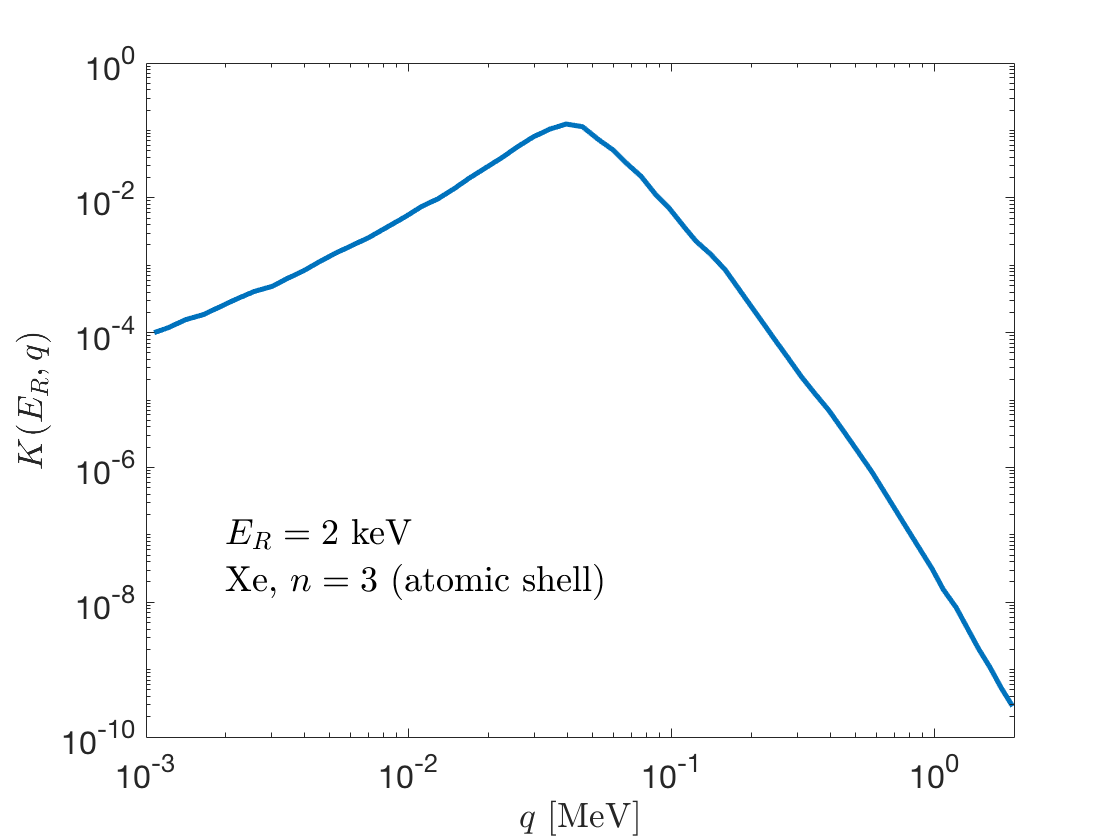
From Eq. (35), the range of the electron recoil energy is

$$E_{R}^{\pm}\simeq\Delta m\left(1\pm\sqrt{\frac{2m_{e}v^{2}}{\Delta m}}\right),$$

(38)

and the differential cross-section in this range becomes

$$\frac{d\langle\sigma v\rangle}{dE_{R}}=\frac{\bar{\sigma}_{e}}{2m_{e}}K^{\prime}(E_{R})\int_{0}^{v_{\rm max}}\frac{f(v)}{v}dv~\Theta(E_{R}-E_{R}^{-})\Theta(E_{R}^{+}-E_{R}),$$

(39)

where for $E_{R}^{+}-E_{R}^{-}\ll E_{R}^{\pm}$, and where $\Theta(E_{R}-E_{R}^{-})\Theta(E_{R}^{+}-E_{R})\simeq(E_{R}^{+}-E_{R}^{-})\delta(E_{R}-\Delta m)$. Thus we have

$$\frac{d\langle\sigma v\rangle}{dE_{R}}=\sqrt{\frac{2\Delta m}{m_{e}}}\bar{\sigma}_{e}K^{\prime}(E_{R})\delta(E_{R}-\Delta m)\int_{0}^{v_{\rm max}}f(v)dv.$$

(40)

Note that for $v_{\rm max}=\sqrt{2\Delta m/m_{e}}\gg v_{0}$ (the most probable velocity), we get $\int_{0}^{v_{\rm max}}f(v)dv\simeq 1$. In practice, the electron recoil energy is not manifested as a Dirac delta function but rather smeared by the detector resolution. This can be modeled by [1]

$$\sigma_{r}=a\sqrt{E_{R}}+b~E_{R},$$

(41)

with $a=(0.310\pm 0.004)\sqrt{\text{keV}}$ and $b=0.0037\pm 0.0003$. We assume the resolution function is a Gaussian of the form

$$R_{S}(E,E_{R})=\frac{1}{\sqrt{2\pi}\sigma_{r}}\exp\left[-\frac{(E-E_{R})^{2}}{\sigma^{2}_{r}}\right]~\alpha(E),$$

(42)

where $\alpha(E)$ is the efficiency given in Fig. 2 of Ref. [1] which we take to be 0.8 for our purposes. As a result, the DM detection rate is

	$\displaystyle\frac{dR}{dE}$	$\displaystyle=n_{\rm Xe}\frac{\rho_{2}}{m_{2}}\int\frac{d\langle\sigma v\rangle}{dE_{R}}R_{S}(E,E_{R})dE_{R}$
		$\displaystyle=n_{\rm Xe}~\rho_{2}\sqrt{\frac{2\Delta m}{m_{e}}}\frac{\bar{\sigma}_{e}}{m_{2}}K^{\prime}(\Delta m)R_{S}(E,\Delta m),$		(43)

where $n_{\rm Xe}\simeq 4.2\times 10^{27}/$ton is the number of xenon atoms in the detector and $\rho_{2}\simeq 0.15$ GeV/cm³ assuming that $D_{2}^{\prime}$ makes half the amount of the observed relic density. At the recoil energy of interest, $E_{R}\simeq\Delta m\simeq 2.5$ keV and $K^{\prime}(\Delta m)\simeq 19.4$. The event detection rate becomes

$$\frac{dR}{dE}\simeq(1.5\times 10^{45}~\text{GeV/cm}^{2})\frac{\bar{\sigma}_{e}}{m_{2}}R_{S}(E,\Delta m),$$

(44)

which has units of $(\text{t}\cdot\text{yr}\cdot\text{keV})^{-1}$.

Using Eq. (44) we attempt to fit the theory predictions of the model based on the benchmarks (a), (b) and (c) of Table 1 to the Xenon-1T data. But before doing so, let us discuss the stringent experimental constraints that must be satisfied.

Those constraints are summarized in Fig. 3. Here CRESST-III (2019) [53] gives the most sensitive limits on the DM-nucleon scattering for the light mass range, 0.1$-$10 GeV. The DM-nucleon scattering cross-section against a nucleus with mass number $A$ and proton number $Z$ can be written as

$$\sigma_{N}=\frac{g_{X}^{2}(Q_{1}+Q_{2})^{2}g_{2}^{2}v_{f}^{\prime 2}}{16\pi\cos^{2}\theta}\frac{\mu^{2}_{DN}}{m^{4}_{\gamma^{\prime}}}\left(\frac{Z}{A}\right)^{2},$$

(45)

where $\mu_{DN}$ is the DM-nucleon reduced mass and $Z/A\sim 0.5$.

Dark photon experiments [54] such as CHARM set limits on visible and invisible decays of the dark photon. These limits are shown in the kinetic mixing-dark photon mass plane in the top panels of Fig. 3 for benchmarks (a) (left), (b) (center) and (c) (right) recast to our model parameters. Also shown are the SuperCDMS [55] sensitivity projections for benchmarks (a) and (b) while (c) remains out of reach of SuperCDMS. In the bottom panels, we present the recast limits from the Planck experiment [56, 57] for the same benchmarks in the gauge coupling $g_{X}$-dark photon mass plane. These limits pertain to the annihilation of DM to two new vector bosons followed by their decay to two $e^{+}e^{-}$ pairs. The benchmarks of Table 1 satisfy all of the above constraints. There is a larger parameter space than the benchmarks of Table 1 where the experimental limits can be evaded while satisfying the relic density and producing the correct fit to the Xenon-1T excess. We exhibit those regions in the top panels of Fig. 3. The green patches show the parts of the parameter space giving the correct DM relic density for a specific choice of the dark coupling $g_{X}$ and the grey stripes indicate the regions producing the correct fit to the Xenon-1T excess.

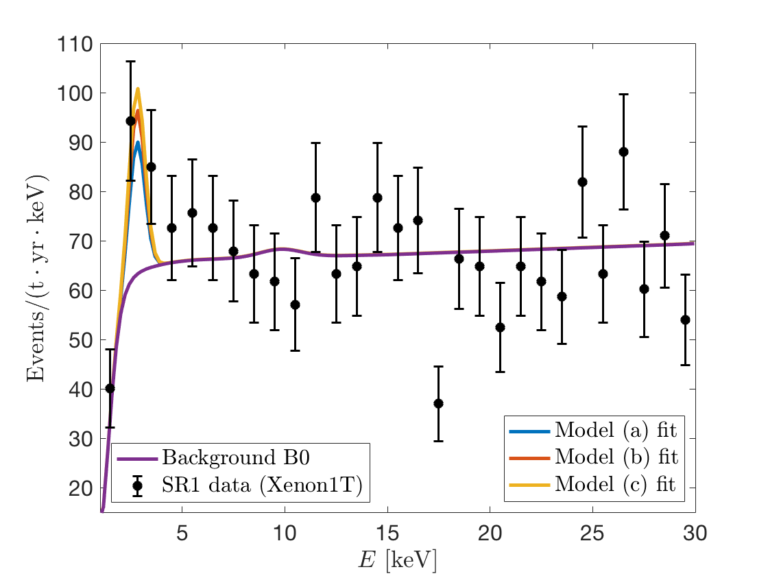
We exhibit in Fig. 4 the Xenon-1T data points (SR1) for the electron recoil events in the detector along with the background-only hypothesis (B0). The event rates for the three benchmarks in our model are plotted over the background showing a clear enhancement near 2.5$-$2.8 keV as expected. Lighter DM particles give a larger event rate since the latter is dependent on $\bar{\sigma}_{e}/m_{2}$. Thus more data in the future which can measure the height of the peak more accurately can determine more precisely the allowed range of the dark matter mass.

In this work we have investigated the Xenon-1T signal as arising from sub-GeV hidden sector dark matter. Specifically we consider a $U(1)$ Stueckelberg extension of the Standard Model with two dark Dirac fermions degenerate in mass charged under the $U(1)$ gauge group. The fermion mass degeneracy is broken by a small mass mixing term which removes the degeneracy and produces two Dirac fermions $D_{1}^{\prime},D_{2}^{\prime}$ where $D_{2}^{\prime}$ is heavier than $D_{1}^{\prime}$ with a mass splitting size $\sim$ 3 keV. The observed effect is explained by the exothermic inelastic scattering $eD_{2}^{\prime}\to eD_{1}^{\prime}$. The scattering occurs via exchange of a dark photon which is the massive gauge boson of the hidden sector. The coupling of the dark photon to the electron arises from gauge kinetic mixing of the $U(1)$ gauge boson of the hidden sector with the gauge boson of the $U(1)_{Y}$ hypercharge. In the work here we have given a detailed analysis of the dark matter relic density constituted of dark fermions while the dark photons decay before the BBN time. As noted above there are two dark fermions in the system $D_{1}^{\prime}$ and $D_{2}^{\prime}$ where $D_{2}^{\prime}$ has a mass slightly greater than that of $D_{1}^{\prime}$ and decays to $D_{1}^{\prime}$ via the channel $D^{\prime}_{2}\to D_{1}^{\prime}+\nu\bar{\nu}$. However, the lifetime for this decay is larger than the age of the universe and so for all practical purposes dark matter is constituted of two dark fermions $D_{2}^{\prime}$ and $D_{1}^{\prime}$ in essentially equal amount. In the analysis of the relic density one encounters stringent constraints on kinetic mixing and on the dark photon mass from CRESST 2019 DM-nucleon scattering cross section, and from the CHARM experiment. We have translated these constraints for our analysis for the model points considered in Table 1 and show that the model parameters of Table 1 are consistent with these constraints (Fig. 3). We note in passing that these constraints, i.e., on the kinetic mixing and on the dark photon mass, are projected to become more stringent from future data from SuperCDMS as shown in Fig. 3 putting further constraints on the allowed parameter space of GeV size dark matter models. Further, the Planck experiment gives constraints on the $U(1)_{X}$ gauge coupling and the dark photon mass from the dark matter annihilation to $4e$ which arise in our case from the annihilation channel $D^{\prime}\bar{D}^{\prime}\to\gamma^{\prime}\gamma^{\prime}\to 4e$. Here again we show that our model is consistent with these constraints as exhibited in Fig. 3.

In Fig. 4 we showed that the models listed in Table 1, which satisfy all the known constraints on kinetic mixing, on the gauge coupling of the $U(1)_{X}$ of the dark sector, on the dark photon mass, and generate relic density of dark matter consistent with the Planck experiment, can explain the Xenon-1T excess. We noted that the size of the peak for the excess events is model-dependent and more data in the future from the Xenon-1T collaboration will help delineate the nature of the dark sector more accurately. Further checks on the model can also come from additional data from the direct detection experiments that focus on the low mass region of dark matter in the GeV region.

In this appendix we give further details of the analysis presented in the main body of the paper. Thus in appendix A we discuss the generation of the mass term for the $D_{1}$ and $D_{2}$ quarks and of the mixing term involving $\bar{D}_{1}D_{2}+\bar{D}_{2}D_{1}$ from a Higgs mechanism. In appendix B we give the cross-sections for the annihilation of $D\bar{D}$ into $q\bar{q},\ell\bar{\ell}$, $\nu\bar{\nu}$ and $\gamma^{\prime}\gamma^{\prime}$ and the cross section for the conversion process $D_{2}\bar{D}_{2}\to D_{1}\bar{D}_{1}$. In appendix C details of the partial decay widths of the dark photon $\gamma^{\prime}$ are given, i.e., $\gamma^{\prime}\to\ell\bar{\ell},q\bar{q},\nu\bar{\nu}$.

References

- [1] E. Aprile et al. [XENON], Phys. Rev. D 102, no.7, 072004 (2020) doi:10.1103/PhysRevD.102.072004 [arXiv:2006.09721 [hep-ex]].
- [2] N. Viaux, M. Catelan, P. B. Stetson, G. Raffelt, J. Redondo, A. A. R. Valcarce and A. Weiss, Phys. Rev. Lett. 111, 231301 (2013) doi:10.1103/PhysRevLett.111.231301 [arXiv:1311.1669 [astro-ph.SR]].
- [3] M. M. Miller Bertolami, B. E. Melendez, L. G. Althaus and J. Isern, JCAP 10, 069 (2014) doi:10.1088/1475-7516/2014/10/069 [arXiv:1406.7712 [hep-ph]].
- [4] T. Battich, A. H. Córsico, L. G. Althaus, M. M. Miller Bertolami and M. M. M. Bertolami, JCAP 08, 062 (2016) doi:10.1088/1475-7516/2016/08/062 [arXiv:1605.07668 [astro-ph.SR]].
- [5] M. Giannotti, I. G. Irastorza, J. Redondo, A. Ringwald and K. Saikawa, JCAP 10, 010 (2017) doi:10.1088/1475-7516/2017/10/010 [arXiv:1708.02111 [hep-ph]].
- [6] S. Shakeri, F. Hajkarim and S. S. Xue, [arXiv:2008.05029 [hep-ph]].
- [7] V. V. Khruschov, [arXiv:2008.03150 [hep-ph]].
- [8] G. Arcadi, A. Bally, F. Goertz, K. Tame-Narvaez, V. Tenorth and S. Vogl, [arXiv:2007.08500 [hep-ph]].
- [9] A. N. Khan, Phys. Lett. B 809, 135782 (2020) doi:10.1016/j.physletb.2020.135782 [arXiv:2006.12887 [hep-ph]].
- [10] J. Cao, X. Du, Z. Li, F. Wang and Y. Zhang, [arXiv:2007.09981 [hep-ph]].
- [11] F. Takahashi, M. Yamada and W. Yin, [arXiv:2007.10311 [hep-ph]].
- [12] A. Karozas, S. F. King, G. K. Leontaris and D. K. Papoulias, [arXiv:2008.03295 [hep-ph]].
- [13] L. A. Anchordoqui, I. Antoniadis, K. Benakli and D. Lust, Phys. Lett. B 810, 135838 (2020) doi:10.1016/j.physletb.2020.135838 [arXiv:2007.11697 [hep-th]].
- [14] Y. Jho, J. C. Park, S. C. Park and P. Y. Tseng, Phys. Lett. B 811, 135863 (2020) doi:10.1016/j.physletb.2020.135863 [arXiv:2006.13910 [hep-ph]].
- [15] B. Fornal, P. Sandick, J. Shu, M. Su and Y. Zhao, Phys. Rev. Lett. 125, no.16, 161804 (2020) doi:10.1103/PhysRevLett.125.161804 [arXiv:2006.11264 [hep-ph]].
- [16] L. Delle Rose, G. Hütsi, C. Marzo and L. Marzola, [arXiv:2006.16078 [hep-ph]].
- [17] M. Millea, [arXiv:2007.05659 [astro-ph.CO]].
- [18] F. Arias-Aragon, F. D’Eramo, R. Z. Ferreira, L. Merlo and A. Notari, [arXiv:2007.06579 [hep-ph]].
- [19] H. N. Long, D. V. Soa, V. H. Binh and A. E. Cárcamo Hernández, [arXiv:2007.05004 [hep-ph]].
- [20] P. Athron, C. Balázs, A. Beniwal, J. E. Camargo-Molina, A. Fowlie, T. E. Gonzalo, S. Hoof, F. Kahlhoefer, D. J. E. Marsh and M. T. Prim, et al. [arXiv:2007.05517 [astro-ph.CO]].
- [21] T. Li, [arXiv:2007.00874 [hep-ph]].
- [22] C. Cai, H. H. Zhang, M. T. Frandsen, M. Rosenlyst and G. Cacciapaglia, Phys. Rev. D 102, no.7, 075018 (2020) doi:10.1103/PhysRevD.102.075018 [arXiv:2006.16267 [hep-ph]].
- [23] C. Gao, J. Liu, L. T. Wang, X. P. Wang, W. Xue and Y. M. Zhong, Phys. Rev. Lett. 125, no.13, 131806 (2020) doi:10.1103/PhysRevLett.125.131806 [arXiv:2006.14598 [hep-ph]].
- [24] C. W. Chiang and B. Q. Lu, [arXiv:2007.06401 [hep-ph]].
- [25] G. Choi, T. T. Yanagida and N. Yokozaki, Phys. Lett. B 810, 135836 (2020) doi:10.1016/j.physletb.2020.135836 [arXiv:2007.04278 [hep-ph]].
- [26] N. Okada, S. Okada, D. Raut and Q. Shafi, Phys. Lett. B 810, 135785 (2020) doi:10.1016/j.physletb.2020.135785 [arXiv:2007.02898 [hep-ph]].
- [27] S. Baek, J. Kim and P. Ko, Phys. Lett. B 810, 135848 (2020) doi:10.1016/j.physletb.2020.135848 [arXiv:2006.16876 [hep-ph]].
- [28] Y. Gao and T. Li, [arXiv:2006.16192 [hep-ph]].
- [29] M. Lindner, Y. Mambrini, T. B. d. Melo and F. S. Queiroz, [arXiv:2006.14590 [hep-ph]].
- [30] J. Bramante and N. Song, Phys. Rev. Lett. 125, no.16, 161805 (2020) doi:10.1103/PhysRevLett.125.161805 [arXiv:2006.14089 [hep-ph]].
- [31] D. Aristizabal Sierra, V. De Romeri, L. J. Flores and D. K. Papoulias, Phys. Lett. B 809, 135681 (2020) doi:10.1016/j.physletb.2020.135681 [arXiv:2006.12457 [hep-ph]].
- [32] K. Harigaya, Y. Nakai and M. Suzuki, Phys. Lett. B 809, 135729 (2020) doi:10.1016/j.physletb.2020.135729 [arXiv:2006.11938 [hep-ph]].
- [33] N. F. Bell, J. B. Dent, B. Dutta, S. Ghosh, J. Kumar and J. L. Newstead, Phys. Rev. Lett. 125, no.16, 161803 (2020) doi:10.1103/PhysRevLett.125.161803 [arXiv:2006.12461 [hep-ph]].
- [34] M. Du, J. Liang, Z. Liu, V. Tran and Y. Xue, [arXiv:2006.11949 [hep-ph]].
- [35] S. Chakraborty, T. H. Jung, V. Loladze, T. Okui and K. Tobioka, [arXiv:2008.10610 [hep-ph]].
- [36] D. Borah, S. Mahapatra, D. Nanda and N. Sahu, [arXiv:2007.10754 [hep-ph]].
- [37] A. Bally, S. Jana and A. Trautner, Phys. Rev. Lett. 125, no.16, 161802 (2020) doi:10.1103/PhysRevLett.125.161802 [arXiv:2006.11919 [hep-ph]].
- [38] J. Kim, T. Nomura and H. Okada, Phys. Lett. B 811, 135862 (2020) doi:10.1016/j.physletb.2020.135862 [arXiv:2007.09894 [hep-ph]].
- [39] Y. Farzan and M. Rajaee, [arXiv:2007.14421 [hep-ph]].
- [40] D. Choudhury, S. Maharana, D. Sachdeva and V. Sahdev, Phys. Rev. D 103, no.1, 015006 (2021) doi:10.1103/PhysRevD.103.015006 [arXiv:2007.08205 [hep-ph]].
- [41] K. S. Babu, S. Jana and M. Lindner, JHEP 10, 040 (2020) doi:10.1007/JHEP10(2020)040 [arXiv:2007.04291 [hep-ph]].
- [42] F. Bergsma et al. [CHARM], Phys. Lett. B 166, 473-478 (1986) doi:10.1016/0370-2693(86)91601-1
- [43] S. N. Gninenko, Phys. Lett. B 713, 244-248 (2012) doi:10.1016/j.physletb.2012.06.002 [arXiv:1204.3583 [hep-ph]].
- [44] B. Holdom, Phys. Lett. B 166, 196-198 (1986) doi:10.1016/0370-2693(86)91377-8; Phys. Lett. B 259, 329 (1991). doi:10.1016/0370-2693(91)90836-F
- [45] B. Kors and P. Nath, Phys. Lett. B 586, 366-372 (2004) doi:10.1016/j.physletb.2004.02.051 [arXiv:hep-ph/0402047 [hep-ph]]; JHEP 07, 069 (2005) doi:10.1088/1126-6708/2005/07/069.
- [46] K. Cheung and T. C. Yuan, JHEP 03, 120 (2007) doi:10.1088/1126-6708/2007/03/120 [arXiv:hep-ph/0701107 [hep-ph]].
- [47] D. Feldman, Z. Liu and P. Nath, Phys. Rev. D 75, 115001 (2007) doi:10.1103/PhysRevD.75.115001 [arXiv:hep-ph/0702123 [hep-ph]]; Phys. Rev. D 79, 063509 (2009) doi:10.1103 /PhysRevD.79.063509.
- [48] L. J. Hall, K. Jedamzik, J. March-Russell and S. M. West, JHEP 03, 080 (2010) doi:10.1007/JHEP03(2010)080 [arXiv:0911.1120 [hep-ph]].
- [49] A. Aboubrahim, W. Z. Feng, P. Nath and Z. Y. Wang, [arXiv:2008.00529 [hep-ph]].
- [50] N. Aghanim et al. [Planck], Astron. Astrophys. 641, A6 (2020) doi:10.1051/0004-6361/201833910 [arXiv:1807.06209 [astro-ph.CO]].
- [51] H. M. Lee, [arXiv:2006.13183 [hep-ph]].
- [52] B. M. Roberts and V. V. Flambaum, Phys. Rev. D 100, no.6, 063017 (2019) doi:10.1103/PhysRevD.100.063017 [arXiv:1904.07127 [hep-ph]].
- [53] A. H. Abdelhameed et al. [CRESST], Phys. Rev. D 100, no.10, 102002 (2019) doi:10.1103/PhysRevD.100.102002 [arXiv:1904.00498 [astro-ph.CO]].
- [54] R. Essig, J. A. Jaros, W. Wester, P. Hansson Adrian, S. Andreas, T. Averett, O. Baker, B. Batell, M. Battaglieri and J. Beacham, et al. [arXiv:1311.0029 [hep-ph]].
- [55] R. Agnese et al. [SuperCDMS], Phys. Rev. D 95, no.8, 082002 (2017) doi:10.1103/PhysRevD.95.082002 [arXiv:1610.00006 [physics.ins-det]].
- [56] P. A. R. Ade et al. [Planck], Astron. Astrophys. 594, A13 (2016) doi:10.1051/0004-6361/201525830 [arXiv:1502.01589 [astro-ph.CO]].
- [57] T. R. Slatyer, Phys. Rev. D 93, no.2, 023527 (2016) doi:10.1103/PhysRevD.93.023527 [arXiv:1506.03811 [hep-ph]].