Probing Saraswati’s heart: evaluating the dynamical state of the massive galaxy cluster A2631 through a comprehensive weak-lensing and dynamical analysis2018Probing Saraswati’s heart: evaluating the dynamical state of the massive galaxy cluster A2631 through a comprehensive weak-lensing and dynamical analysis–References
Abstract
In this work, we investigate the dynamical state of the galaxy cluster Abell 2631, a massive structure located at the core of the Saraswati supercluster. To do this, we first solve a tension found in the literature regarding the weak-lensing mass determination of the cluster. We do this through a comprehensive weak-lensing analysis, exploring the power of the combination of shear and magnification data sets. We find M⊙. We also determined the mass based on the dynamics of spectroscopic members, corresponding to M⊙, consistent within a 68 per cent CL with the weak-lensing estimate. The scenarios provided by the mass distribution and dynamics of galaxies are reconciled with those provided by X-ray observations in a scenario where A2631 is observed at a late stage of merging.
Keywords:
gravitational lensing: weak – dark matter – clusters: individual: Abell 2631 – large-scale structure of Universe1 Introduction
At the largest scales, the matter distribution of the Universe matches a web-like structure surrounded by voids where the density is particularly low (Springel et al. 2018, e.g.). This picture has been designed across time by the gravitational interaction within the context of the hierarchical scenario, where the largest structures are formed late through the merger of the smallest. In this context, superclusters of galaxies constitute the next generation of the most massive large-scale structures in the Universe (Lacey & Cole 1993; Kravtsov & Borgani 2012, e.g.).
The supercluster Saraswati was discovered by Bagchi et al. 2017 in the Stripe 82 region of the Sloan Digital Sky Survey (York et al. 2000, SDSS;). It forms a wall-like structure covering 200 Mpc at . The main body of the supercluster comprises at least 43 galaxy clusters or groups with a total mass of , which includes at least 23 massive galaxy clusters of according to the mass-richness relation. This implies a peculiar high-mass concentration since only massive galaxy clusters are expected within Saraswati’s whole volume according to the excursion set approach (Sheth et al. 2001). The bound core ( Mpc) is composed of five high-mass galaxy clusters. These properties place Saraswati among the few largest and most massive superclusters known, comparable to the most massive ‘Shapley Concentration’ or ‘Shapley Attractor’ () in the nearby universe (Melnick & Moles 1987; Scaramella et al. 1989; Raychaudhury 1989).
Due to a whole range of matter overdensities present in the cosmic web, ranging from rarified voids, intermediate-mass filaments and groups to highly overdense massive galaxy clusters, this supercluster offers exciting possibilities for several promising studies, and one such method is the gravitational weak-lensing mapping of dark matter distributed in the vast supercluster environment, which has rarely been attempted. Such studies provide a good understanding of what physical processes were involved in the growth of such enormous cosmic structures in the distant universe ( Gyr lookback time) when mysterious dark energy had just started to dominate structure formation.
At the very centre of the bound core, or the ‘heart’ of Saraswati, is located the most massive cluster member, Abell 2631 (), which is an extremely rich (Abell richness class ), massive () and hot ( KeV) galaxy cluster (Bagchi et al. 2017). This cluster is the subject matter of our present paper.
Abell 2631, also known as RXCJ 2337.6+0016 (hereafter A2631), has been studied through several wavelengths. For example, using XMM-Newton data, Finoguenov et al. 2005 noticed that the intracluster medium (ICM) shows elongated innermost X-ray isophotes, although they appear symmetric at larger radii. They observed a relatively high central entropy for the ICM, suggesting that A2631 is a galaxy cluster in the late stage of a merger. Similar conclusions were drawn by Zhang et al. 2006 that classified A2631 as an “offset centre” cluster due to the non-concentric X-ray isophotes. They also confirmed the high mass of A2631, estimating M⊙. All previous statements were also endorsed by high-resolution data observed by Chandra (Mann & Ebeling 2012; Marrone et al. 2012).
Considering now the other end of the electromagnetic spectrum, observations taken by the Giant Metrewave Radio Telescope (Swarup et al. 1991, GMRT;) at 610 MHz did not reveal any signal of extended radio emission in A2631 (Venturi et al. 2007), which was subsequently ratified by Knowles et al. 2019. Radio halos are expected to appear as signatures of massive cluster mergers (Feretti et al. 2002). A2631 was also observed with the Sunyaev–Zel’dovich Array (SZA) by Reese et al. 2012, which estimated M⊙. Also using Chandra images, they corroborate the scenario of an elongated core both in X-ray and SZA data. However, the authors did not found any signals of substructures, which are proxies for disturbed systems (Andrade-Santos et al. 2012) nor a cool core, which is expected in relaxed clusters (Soja et al. 2018, e.g.). The dynamical state of A2631 so far remains an unsolved puzzle.
Despite X-ray and radio exhibiting the most dramatic signatures of a cluster merger (Feretti et al. 2002; Markevitch & Vikhlinin 2007), this process leaves few imprints in the cluster optical properties (Pinkney et al. 1996, e.g.). Within this context, Wen & Han 2013 developed a new methodology to attest to a cluster’s dynamical state based only on the brightness distribution of member galaxies. They defined a relaxation parameter cut-off that satisfactorily separates the relaxed () and unrelaxed () systems with a success rate of 94 per cent. Unfortunately, they found an inconclusive classification for A2631 ().
The mass of a galaxy cluster is a fundamental parameter to probe theoretical models of large-scale structure formation and evolution as well as to constrain cosmological parameters (Kravtsov & Borgani 2012; Pratt et al. 2019, e.g.). Due to its unusual high mass, A2631 has been a popular target for mass surveys based on gravitational lensing. We can cite the Local Cluster Substructure Survey (Zhang et al. 2008; Haines et al. 2009, LoCuSS11 1 http://www.sr.bham.ac.uk/locuss/; e.g.) that has been analysing 50 of the most massive galaxy clusters in the local universe aiming to determine their masses as accurately as possible. Another remarkable example is the project Weighing the Giants (von der Linden et al. 2014; Applegate et al. 2014, WtG;). The main advantage of lensing-based mass determinations is that they do not assume any prior about the cluster dynamical state, in contrast to other techniques do. For example, X-ray hydrostatic mass estimators rely on the assumption of hydrostatic equilibrium in the innermost cluster region (). Therefore the masses obtained will be highly biased in merging systems.
We present the multiwavelength mass estimates of A2631 in Table 1. A comparison of masses obtained from different techniques is an important tool to probe the dynamical state of a galaxy cluster (Cypriano et al. 2004, e.g.). However, we observe a tension among the weak-lensing masses available in the literature. The values vary within a range of [4–17] M⊙ (disregarding the error bars) leading to a discrepancy of a factor of . Such inconsistency can bias the statistic of cluster masses to cosmological purposes and affect the scaling relations with observables (e.g. SZ, X-ray, richness).
| Method | Reference | ||
| M | (Mpc) | ||
| caustic | Geller et al. 2013 | ||
| caustic | Maughan et al. 2016 | ||
| dynamic | Sifón et al. 2016 | ||
| MRR | Bagchi et al. 2017 | ||
| WGL | Okabe et al. 2010 | ||
| WGL | Applegate et al. 2014 | ||
| WGL | Okabe & Smith 2016 | ||
| WGL | Klein et al. 2019 | ||
| SZ | Hasselfield et al. 2013 | ||
| SZ | Planck Collaboration & Ade 2013 | ||
| X–ray | Zhang et al. 2006 | ||
| X–ray | Landry et al. 2013 | ||
| X-ray | Maughan et al. 2016 |
These inconsistencies encouraged us to conduct a comprehensive optical study of A2631 with the aim of (1) solving the discrepancy in the weak-lensing mass determination and (2) evaluating its current dynamical status. To reach these goals, we resorted to existing large field-of-view multiband images (, , and ) taken from the Subaru telescope archive as well as available redshift catalogues. With this wealth of data, we mapped the spatial distribution of the cluster’s dark matter and its galaxy content. We reconstructed the cluster mass field combining two different probes of the gravitational lensing effect, the shape distortion induced on the background galaxies and the change in their number counts. This combination contributed to a more precise determination of the cluster’s total mass. We also quantified the statistical significance among the spatial distribution of the cluster components, dark matter, galaxies, and gas. This piece of information works as a proxy for the dynamical state since a highly disturbed system can present a spatial detachment among these quantities (Massey et al. 2011; Merten et al. 2011; Pandge et al. 2019; Monteiro-Oliveira et al. 2020; Moura et al. 2021, e.g.). Additionally, we determined the dynamical-based mass and searched for substructures as a probe for the cluster’s dynamical state (Ribeiro et al. 2013, e.g.).
The paper is organized as follows. In Section 2, we present the cluster photometric analysis. The weak-lensing mass reconstruction is performed in Section 3. Next, we describe A2631 from the dynamical point of view in Section 4. The main findings of this work are discussed in Section 5 and summarized in Section 6.
Throughout this paper, we adopt the standard CDM cosmology, represented by , , and . At the mean cluster redshift of , we have a plate-scale of 1 arcsec equals 4.23 kpc (Wright 2006).
2 Photometric analysis
2.1 Imaging data
The galaxy cluster A2631 was observed in multifilters , , by the SuprimeCam22 2 https://www.subarutelescope.org/Observing/Instruments/SCam/index.html mounted at the Subaru telescope33 3 https://www.nao.ac.jp/en/research/telescope/subaru.html on 2004 July 18 ( and ) and 2005 November 30 ()44 4 smoka.nao.ac.jp. Details about the final products can be found in Table 2.
| Band | Exposure time | Seeing |
|---|---|---|
| (min) | (arcsec) | |
| 12 | 1.0 | |
| 18 | 0.8 | |
| 24 | 0.8 |
The image reduction was done with the standard semi-automated code SDFRED1 (Ouchi et al. 2004). The steps consisted of bias and overscan subtraction55 5 These auxiliary images are also available at the SMOKA Science Archive., flat-fielding, atmospheric and dispersion correction, sky subtraction, auto-guide masking, and alignment (which was done simultaneously in all filters). Then, single images were combined and mosaicked into a final image for each filter. To ensure the exact correspondence among their Cartesian components (, ), we performed their joint registration with IRAF. The size of the final images was arcmin2, sufficient to map large projected distances from the centre of A2631 as required to perform a safe weak-lensing analysis.
Astrometric calibration was done based on the comparison of precise positions of bright and unsaturated stars from the “Fourth US Naval Observatory CCD Astrograph Catalog” (Zacharias et al. 2013, UCAC4;) and in our images. After this process, we found a positional rms of arcsec, thus ensuring a satisfactory accuracy for our forthcoming analysis.
In order to perform the photometric calibration, i.e., to transform the measured fluxes into the AB magnitude system (Oke 1974), we need to observe some standard field (stars with known AB magnitudes) over several (or at least two) air masses on the same date as the science observations. For our data set, only the filter matches this requirement. We determined the extinction coefficients and through the following relation,
| (1) |
with being the reference AB magnitude, the instrumental magnitude, the airmass, the AB index colour (e.g. ), and a calibration constant. Then a low-exposure science image was calibrated also taking into account the factor where is the ratio between the time exposure of the science (240 s) and the standard star (10 s) images. To estimate , we adopted the index colour of the galaxy type located at (Fukugita et al. 1995). Then we compared this calibrated image with the co-added image. We found the magnitude zero-point .
To calibrate the filter , we turn to SDSS DR12 (Alam et al. 2015) to find the calibration coefficients and for the single standard field observed, as given by the linear fit
| (2) |
Following this, and were applied to calibrate a low-exposure science image that served as the base to the photometric calibration of the co-added image. The magnitude zero-point obtained is . A similar procedure was done for filter, except that we did not have any standard field from the same date as the science observations. We overcome this issue obtaining and by comparing the SDSS DR12 catalogue with the catalogue of A2034 (Monteiro-Oliveira et al. 2018). We found .
Photometric catalogues were created using SExctractor (Bertin & Arnouts 1996) in double mode with the deepest image as a base. Galaxies were identified according to two complementary criteria. For the brightest objects () galaxies will correspond to whereas for their full width at half-maximum (FWHM) should be greater than arcsec. This value is arcsec larger than the seeing to ensure the selection of well resolved objects.
2.2 Identification of the red-sequence
The central region of rich galaxy clusters is inhabited preferentially by red members (Dressler 1980). As a result of the homogeneous photometric properties, these galaxies occupy a well defined locus in a colour-colour map (Medezinski et al. 2018, CC; e.g.). Here, we identified the red-sequence locus of A2631 on the versus space applying the statistical subtraction method (see Monteiro-Oliveira et al. 2017b, for more details).
We selected 964 photometric members over the field within . This corresponds to the faintest limit where galaxy counts in the innermost region are higher than those in the outskirts, where field counts are expected to dominate. The red-sequence projected density weighted by the flux is shown in Fig. 1. The map shows the results of the smoothing of photometric members inside a arcsec2 cell by an Epanechnikov kernel with a scale of 70 arcsec.

The luminosity spatial distribution is dominated by the brightest cluster galaxy (BCG) and some luminous neighbours. A2631 is well described by a single structure just as the majority of relaxed clusters are (Wen & Han 2013). Next, we will recover the cluster projected mass distribution in order to check if this scenario is supported.
3 weak-lensing analysis
3.1 Basic concepts
We can approach the effects of the gravitational lens from the projection of its scalar potential,
| (3) |
This is conveniently defined so that we can directly write
| (4) |
with
| (5) |
being the projected mass density of the lens also known as convergence. It is written in units of the lensing critical density
| (6) |
where , , and are, respectively, the angular diameter distances to the source, between the lens and the source, and to the lens.
Besides the scalar convergence, the gravitational lensing field can be described by a spin-2 tensor, the shear
| (7) |
whose components are both second derivatives of the projected gravitational potential (Equation 3). An alternative way to define these quantities is in terms of their tangential component to the lens centre and another one in relation to that, .
In the absence of any gravitational lens, the value of the averaged ellipticities of background66 6 With respect to the targeted galaxy cluster. galaxies is expected to be zero. However, the lens effect acts to induce a coherent distortion whose averaged ellipticity will tend to the effective shear :
| (8) |
As , the full ellipticity, and the effective shear are both a spin-2 tensor. Mathematically the weak regime corresponds to . In this case, we have .
During the passage through the gravitational lens, there is conservation of the angular momentum and energy of the photons coming from the background galaxies. Considering also the absence of emitters and absorbers in the path of the light beam from the source to the observer, we conclude that there is numeric conservation of the photons. From Liouville’s theorem, we can enunciate an important characteristic of the phenomenon of gravitational lensing: the conservation of surface brightness. Due to the amplification of the image size, the observed flux (superficial brightness the image’s solid angle) will be increased by the same factor implying that the lensed image will be brighter than its source. This increase is quantified by the magnification :
| (9) |
Parallel to the reconstruction of the mass distribution of the measured lens from the measurement of the distortion caused in the background galaxies, it is possible to do the same work from the measurement of the magnification effect caused locally in the spatial distribution of background galaxies.
The so-called “magnification bias” is the joint manifestation of two effects of the magnification phenomenon: at the same time that it increases the flux from the source, thus allowing the detection of intrinsically weaker objects, it also magnifies by the same value the element of the projected area of the sky acting to decrease the apparent density of objects.
The magnification bias value is related to both the magnification factor (Equation 9) and the slope
| (10) |
of the intrinsic relationship between the logarithm of the galaxy counts as a function of their magnitudes, measured in a field unaffected by the effect of the lens.
When approaching for a circular lens, the numerical radial density of background galaxies can be written as
| (11) |
where is the intrinsic density of objects measured in a region far enough away to not be affected by the gravitational lens.
The magnification bias is present only if , in which case the numerical increase of the magnified sources is exactly compensated by the apparent expansion of space. For we will see an increase in the density of galaxies while in the regime there will be a decrease in this amount compared to .
Since the magnification bias is not based on any measurement of shape in the galaxies nor does it require knowledge about the original shape, its use instead of the technique based on the measurement of distortion would be obvious. However, in the weak-lens regime (), the ratio between the signal and the noise of both extensions, considering and ,
| (12) |
favours analysis based on distortion in the shape of galaxies (Mellier 1999).
Despite this limitation, mass reconstruction through magnification bias constitutes a test to check consistency in the measurement of masses as this approach to the phenomenon of gravitational lenses is not susceptible to systematic effects from the measurement of the shape of galaxies and point spread function (PSF) correction.
3.2 Shear data set
3.2.1 Source selection
We refer to the background, i.e. those galaxies located at higher redshift than A2631, as the sources because they are the basis for shape and/or numerical density measurements required by the weak gravitational lensing technique. Despite the source galaxies being spatially spread along the field, we can resort to the CC map to identify the loci where the contamination by both foreground and red-sequence galaxies is lower (Capak et al. 2007; Medezinski et al. 2010, e.g.).
Before identifying the source locus in the versus space, we need to draw the foreground location. According to synthetic models of galaxy evolution (Medezinski et al. 2018, e.g.), they tend to be bluer than the red-sequence and form a dense cloud in the CC map. We show, in Fig. 2, the position of the foreground locus after a visual inspection. As a sanity check, we overlaid our spectroscopic sample, which we will describe in more detail in Sec. 4.

We then selected the background locus excluding both red-sequence and foreground regions. Background galaxies are usually classified into blue () or red populations (Medezinski et al. 2018, ; e.g.). This taxonomy is relevant when we are interested in the magnification bias effect, i.e the change in the source counts caused by the gravitational lens (Monteiro-Oliveira et al. 2017a, e.g.). For a shear-based analysis, both samples are indistinguishable.
3.2.2 Shape measurements
The PSF is the combined effect of the atmospheric blurring plus the response of the telescope optics and instrumentation on the image. Fortunately, these effects can be described mathematically leading to an analytical expression of the PSF effects. To build this expression, we identified and analysed the shape of bright and unsaturated stars across the image. They should be exact point-like sources in the absence of the PSF effects and they are, without doubt, unlensed objects.
In order to model the shape parameters (ellipticity components and plus the FWHM), we resort to the Bayesian code im2shape (Bridle et al. 1998). It models star profiles as single Gaussians and, in this case, it does not do any PSF deconvolution. Following this, the discrete values of parameters were spatially interpolated to create a continuous function across the image. This is done by thin plate regression (Nychka et al. 2014, tps;) in the R environment. Aiming to remove obvious outliers, we reapplied tps three times; in each iteration, we removed the objects with the 10 per cent largest absolute residuals. We present, in Fig. 3, the measured stellar ellipticities and their respective residuals.

The averaged ellipticity is and . As in practice, stars are not point sources, all deviations from null values are due to the PSF effect. As illustrated by Fig. 3, our model showed a good match with the data as attested by the very low residuals, for and for .
Now, we should measure the shape parameters of the source galaxies and perform PSF deconvolution to extract the weak-lensing signal. There is also the effect of the unknown original shapes, but this will be treated later. We again use the code im2shape but now it models the galaxies as a sum of Gaussians with an elliptical basis and performs local PSF deconvolution. The final result is a PSF-free catalogue of the galaxy ellipticities and and the respective uncertainties . In addition, we removed all source galaxies with or those showing evidence of blending. Our final source catalogue is composed of 15153 galaxies, leading to a projected density of 13.6 galaxies per arcmin2.
In the weak-lensing context, observational parameters are translated into physical quantities through the critical surface density . As pointed out by Equation 6, we need to know the distribution of the source’s redshift. So, we applied the same colour and magnitude cuts (Sec. 3.2.1) in the photometric redshift catalogue of the Cosmic Evolution Survey (Ilbert et al. 2009, COSMOS;). We found M⊙ kpc-2 and a mean redshift of .
3.2.3 The projected mass distribution
Source galaxies have an intrinsic unknown ellipticity that makes them noisy tracers of the shear field. To take this fact into account, we averaged the quadratic sum of the ellipticity components and in the image outskirts where we suppose the lensing signal is insignificant. We found and therefore consider it as the intrinsic error on the ellipticities.
The field projected mass distribution was recovered by the maximum entropy algorithm (Seitz et al. 1998) implemented in the Bayesian code LensEnt2 (Marshall et al. 2002). The code finds the best solution through the maximization of the evidence based on the comparison between the shear field sampled by source ellipticities with those predicted by the model. Since each galaxy ellipticity induced by the gravitational lens is correlated with the neighbourhood, we should adopt a smoothing scale. This also takes into account the fact that each galaxy is a noisy probe of the shear field. The smoothing is implemented in the code by the intrinsic correlation function (ICF), chosen as a Gaussian filter by us.
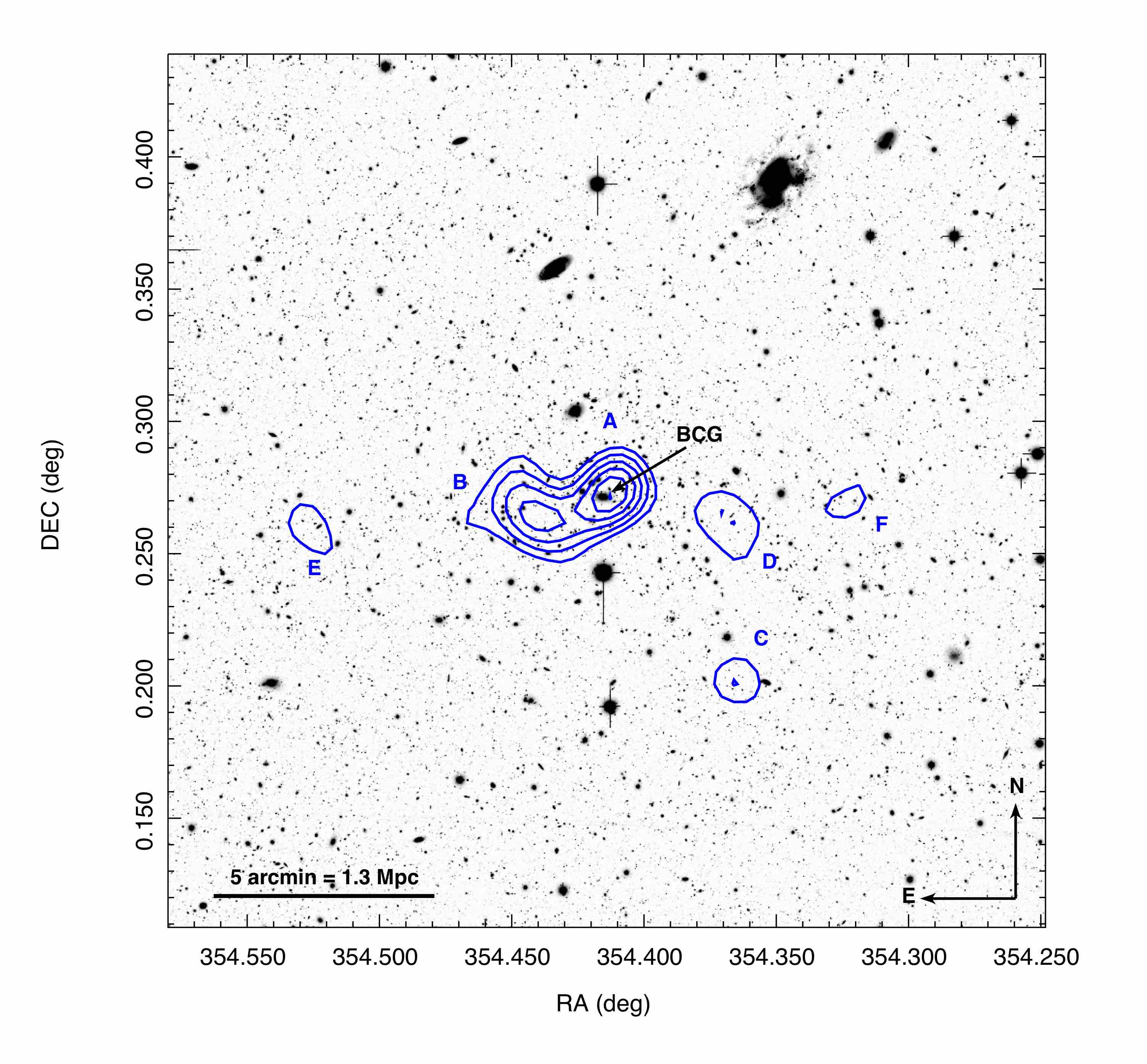
To find the optimized , we made mass reconstructions within the interval [60,120] arcsec. For each, we searched for peaks in mass to compute the statistic of the numeric detections in the function of their significance. We found that peak detections above remain almost constant for arcsec; therefore this value was adopted. The noise level in the convergence map, , was obtained after performing 100 realizations of the shear field without the cluster lens signal. For that, each galaxy ellipticity was rotated by a random angle in the interval [0,180[. We present our fiducial convergence map in Fig. 4. The main characteristics of the convergence map are shown in Table 3.
| (gal. arcmin-2) | 13.6 |
|---|---|
| ICF FWHM (arcsec) | 80 |
| 0.035 |
⋆ Noise level in the convergence map.
The most noticeable feature in the convergence map is the presence of a significant halo matching the BCG position (halo A in Fig. 4). This structure is nearly aligned with the red-sequence spatial distribution (Fig. 1) which allows us to recognize it as the halo of A2631. Also remarkable is the presence of a structure located 1.5 arcmin east of the BCG (halo B). Checking Fig. 1, we did not see any relevant members related to it suggesting that this structure does not belong to our target cluster. Anyway, we will consider this “companion” structure in our forthcoming mass modelling.
3.3 Magnification bias data set
3.3.1 Source selection and counts
Following Monteiro-Oliveira et al. 2017a, we considered only red sources to describe the lens-induced magnification bias. This subsample has a logarithmic slope (Equation 10) computed at the image outskirts 77 7 At least 10 arcmin away from the cluster centre traced by the BCG. near the completeness limit (). Thus, we expect the lensing effect to cause a depletion of the number counts. For this sample, the critical surface density for this sample was estimated in the same way as for the shear data set (Sec. 3.2.1) leading to M⊙ kpc-2 and a mean redshift of .
To map the magnification bias effect, we used the “count-in-cells” technique. We divided our image into squared cells with 1 arcsec per side. Additionally, we masked out regions occupied by large objects as saturated stars and galaxies (including the BCG). Then, we computed the area of each cell after discounting the masked regions. Finally, the counts in regions away from the BCG ( arcmin) yielded a baseline number count of galaxies per arcmin-2.
3.4 Mass modelling
The lensing observables (shear and galaxy counts) were modelled as if they were induced by mass halos following an NFW profile (Navarro et al. 1996; Navarro et al. 1997). For a given set of NFW profile parameters, the shear field was built following Wright & Brainerd 2000 prescriptions. The theoretical profile is defined by four parameters: the lens centre coordinates , the mass enclosed within a radius where the density is 200 the critical density of the Universe88 8 , , and the dimensionless halo concentration . To focus on the determination of the halo centre and its mass, we opt to fix the concentration by adopting the relation presented by Duffy et al. 2008,
| (13) |
where is the cluster redshift.
We are looking for the best model to describe the observed mass distribution in the A2631 field. For this, we computed three different models, described in Table 4. These models were designed to confirm or not whether the other mass clumps found (see in Fig. 4) correspond to substructures of A2631.
| Model | Haloes | |
|---|---|---|
| #1 | 1 (A) | , , |
| #2 | 2 (A, B) | , , , , , |
| #3 | 6 (A–F) | , , , , , , , , , |
We should consider that each source galaxy is simultaneously affected by the computed halos. In this case, we write the effective quantities for a considered galaxy as
| (14) |
with .
For the shear data set we can write the statistic:
| (15) |
where is the predicted reduced shear (Equation 8), is the measured ellipticity and is the shape error given by im2shape.
The log-likelihood for the shear data set can be written as
| (16) |
From the magnification bias view, we can measure the lensing signal by comparing the measured counts with the theoretical prediction as
| (17) |
where corresponds to the cumulative counts in each cell corrected by the unmasked cell area and is a weight that penalizes cells with small effective areas. Then, the log-likelihood is
| (18) |
Following a Bayesian approach, we considered two additional “nuisance parameters” in the models, and , related to the counts of the unlensed population (Sec. 3.3.1). They will be fitted along with the halo-related parameters, but we established normal priors for both based on our measurements. For the masses, we applied a flat prior M⊙, which avoids the consideration of unrealistic values and thus accelerate the convergence of the model. The same strategy was adopted for the halo centres with a prior arcsec (344 kpc), where are the halo centre coordinates.
After these considerations, we can write the posterior of our problem as
| (19) |
where is the vector of parameters.
3.5 Results
The source galaxies considered in our models were restricted to those contained in an area of arcmin2 centred on the BCG. Then, the posterior described in Equation 19 was sampled for each model by the MCMC algorithm with a Metropolis sampler MCMCmetrop1R (Martin et al. 2011). We generated four chains with elements allowing an additional chain of first points in each as “burn-in”.
For the best model selection, we computed the Bayesian information criterion (BIC),
| (20) |
with being the number of model parameters, the number of data points, and is the maximized value of the model’s likelihood. Among a finite number of models, those with the lowest BIC will be preferred. In Table 5, we present a statistical comparison of the models considered.
| Model | Parameters | BIC with respect to model #1 | ||
|---|---|---|---|---|
| s | m | s+m | ||
| #1 | 3 | 0 | 0 | 0 |
| #2 | 6 | 22 | 21 | 20 |
| #3 | 10 | 48 | 55 | 43 |
Concerning the BIC criterion, the lowest index is presented by the simplest model that describes a single-halo at A2631’s location. This description is strongly preferred in relation to the others as indicated by the large value of BIC (Kass & Raftery 1995). Consequently, this will be our fiducial model hereafter.
The parameter estimation based on the analysis of the combined shear and magnification data sets is presented in Table 6. For the sake of comparison, we also show the estimation based on the individual data sets. We considered at face value the median of the respective posterior marginalized over all other parameters (Fig. 5). The error bars correspond to the 68 per cent range of the MCMC samples.
| ( M⊙) | (Mpc) | (deg) | (deg) | |
|---|---|---|---|---|
| s | ||||
| m | ||||
| s+m |

According to our modelling, the galaxy cluster A2631 has a mass of M⊙. From Table 6, we confirm that the analyses based on independent shear and magnification data sets are consistent with each other, having a significant overlap within 1. The combination of both decreased the error bars by 20 per cent in comparison to the shear data set only.
An important proxy for the dynamical state is the detection of possible spatial detachments among the cluster components, dark matter, galaxies, and the ICM. In Fig. 6, we present a close view of A2631 where we can better compare the BCG position (tracer of galaxies distribution), X-ray clump (Ge et al. 2019, tracer of the ICM;) and mass-centre location (tracer of dark matter). The position of the BCG, X-ray, and dark matter clumps are all consistent within the 68 per cent CL. The mass centre is arcsec ( kpc) away from the BCG location and arcsec ( kpc) from the X-ray clump. The BCG and the X-ray peak are 21 arcsec (90 kpc) apart, which is comparable with the Mann & Ebeling 2012 measurement. Therefore, we conclude that all cluster components are centred at a common position within the uncertainties.

4 Dynamical analysis
4.1 Spectroscopic data
A2631 was intensively observed by SDSS (Alam et al. 2015) and the Hectospec Cluster Survey (Rines et al. 2013, HeCS,). In fact, a search on a circular region centred on the BCG and with a radius of 18 arcmin revealed 418 galaxies with available spectroscopic redshifts and with correspondence in our photometric catalogue.
The respective spectroscopic members were selected after application of the clipping method (Yahil & Vidal 1977). This consists of removal of all galaxies beyond the interval , as they are most probably outliers (Wojtak et al. 2007).
The 143 spectroscopic members of A2631 have with a standard deviation of km s-1, corresponding to the inset panel in Fig. 7. According to the Anderson-Darling test (Gross & Ligges 2012) this sample follows, within the 95 % CL, a normal distribution (). This conclusion is also supported by the Hellinger distance estimator (Ribeiro et al. 2013) within the 92 per cent CL The sample extends up to .

4.2 Search for substructures
Even the Gaussianity of the overall redshift distribution does not necessarily mean that the sample is free of substructures. More subtle examples of them (e.g. infalling groups) can pass unscathed through the clipping because they have velocities consistent with those of the general cluster population. To scrutinize the sample, we applied the Dressler-Shectman test (Dressler & Shectman 1988, or -test;). This consists in quantifying the deviation of the local99 9 This means that we consider only the closest neighbours, where is the total number of galaxies in the sample. systemic velocity and dispersion with those of the overall structure,
| (21) |
and computing the statistic
| (22) |
It is expected that (Dressler & Shectman 1988) with a (Hou et al. 2012) for substructured clusters. We found with a (95 % CL) pointing to an absence of substructures in A2631.
The search for substructures based on multidimensional normal mixture modelling was also fruitless. We applied the R-based package MCLUST (Scrucca et al. 2016; Lourenço et al. 2020) in 1D (), 2D ( and ) and 3D (, and ) modes for the spectroscopic members. All of them returned a single group as the best solution, with in relation to the second-best model with two groups. This means that, according to the dynamical view, A2631 is undoubtedly a unimodal structure. The results remain consistent when we consider smaller radii ( and ).
4.3 Dynamical mass
The gravitational potential of the cluster drives the dynamics of its galaxy content. So, we can get the inverse path and estimate the cluster mass from the one-dimensional velocity dispersion since this is an easily measurable observable. In the scope of a virialized system, the virial theorem predicts a theoretical scaling relation in the form with . This scaling relation has been a matter of intense study from the point of view of computational simulations in order to understand the behaviour of “real” systems and then provide a reliable way to determine the cluster mass.
We can rewrite the scaling relation within a radius in a more functional form (Biviano et al. 2006; Evrard et al. 2008; Munari et al. 2013, e.g.),
| (23) |
being 1010 10 Hereafter, and the constants and to be determined. Based on realistic baryon (including cooling, star formation and AGN feedback) plus dark matter simulations, Munari et al. 2013 suggest km s-1 and .
Firstly, we should estimate the unbiased velocity dispersion of cluster members. The “biased” standard deviation is obtained from galaxies inside the projected radius equal to (see Fig. 8). We can correct this for the statistical bias induced by the finite number of galaxies as follows (Ferragamo et al. 2020):
| (24) |
with , , and .

Now, we should correct for the bias induced for three main physical effects: the aperture radius where is measured, the selected fraction of massive galaxies, and contamination by interlopers. In recent work, Ferragamo et al. 2020 presented a comprehensive study regarding statistical properties of velocity dispersion and mass estimators based on simulated galaxy cluster data. The authors suggest a set of multiplicative correction factors to turn , in fact, into an unbiased estimator. We adopted , since we are working with members enclosed within projected , , which corresponds to a fraction of 50%–100% of the massive galaxies in the cluster present in the sample and based on the assumption that the 3 clipping selected sample is contaminated by of interlopers (Wojtak et al. 2007). After these procedures, we found km s-1.
Due to the non-linearity of the relation (Equation 23), even considering an unbiased we will find dependence on in a biased mass estimation, especially for the low regime (Ferragamo et al. 2020, ;). So, we should correct for
| (25) |
with , , , and the “biased” mass given by Equation 23.
The dynamical mass of A2631 is M⊙. This corresponds to a face value per cent larger than the weak-lensing estimated mass (Table 6). However, both mass measurements are consistent within the 68 per cent level. We will resume this discussion in the next section.
5 Discussion
5.1 Weak-lensing mass of A2631
We present here a comprehensive weak-lensing analysis of the massive galaxy cluster A2631 () located at the centre of the Saraswati supercluster. In order to provide an unambiguous estimation of the cluster mass, we reconstructed the mass field combining measurements of shape distortion and magnification bias of the background galaxies. This is a powerful tool because it combines the strengths of both observables: whereas the distortion provides a high S/N, the magnification bias is insensitive to the mass-sheet degeneracy. We based our analysis on large field-of-view ( arcmin2) multiband () Subaru archival images. The source catalogue was carefully selected in the colour-colour space, aiming for a final catalogue as pure as possible (i.e. with minimal contamination by cluster/foreground galaxies). The purity of the source catalogue is essential to preserve the lens-induced signal and then obtain a credible determination of the original mass field.
Our MCMC-based model confirmed that A2631 is a very massive cluster having M⊙. Indeed, according to the Schechter cluster mass function for nearby clusters presented by Girardi et al. 1998, A2631 is among the per cent of most massive clusters with masses above M⊙. The cluster mass corresponds to a halo concentration of according to the relation proposed by Duffy et al. 2008. We also find that the BCG, X-ray emission peak, and mass centre are nearly concentric, all being coincident within the 68 per cent CL. The combination of distortion and magnification bias decreased the uncertainties on the masses to per cent of the distortion-only estimation.
A visual inspection of the convergence map (Fig. 4) can induce the reader to suppose the presence of a companion structure east of A2631. However, this scenario is not supported by either the luminosity-weighted spatial map of the red-sequence galaxies (Fig. 1) or the projected distribution of the spectroscopic members (Fig. 8). Lastly, our mass modelling statistics completely refute any evidence of additional halos in the field. So, what would be the nature of those apparent mass clumps? To answer this question, in Fig. 9 we compare our convergence map with Okabe et al. 2010 and the mass aperture map from von der Linden et al. 2014. The three maps show a dominant mass clump surrounding the BCG. However, a detailed comparison can only be done with Okabe et al. 2010 since von der Linden et al. 2014 shows only the highest-density regions.

Both maps show several structures across the field with most of them found in common (green crosses). Although suggesting a little elongation in the E–W direction when we consider the fewer significative contours, Okabe et al. 2010 did not find a relevant mass neighbour to A2631. So, we conjecture that it arises in our map from the association of small background halos ( M⊙) since they dominate the population in the field (Yang et al. 2013; Liu & Haiman 2016; Wei et al. 2018).
Now, we will compare quantitatively our results with previous weak-lensing-based works. They are presented in Fig. 10 by blue points. Our fiducial mass estimation shows, within the 68 per cent CL, a very good match with Okabe & Smith 2016 and Klein et al. 2019. However, within the same confidence level, the values of Okabe et al. 2010 and von der Linden et al. 2014 are inconsistent with ours.

Among the available weak-lensing mass estimates, Okabe et al. 2010 present the lowest value. Checking the work we found that the authors had only two bands ( and ) to select the sources. Despite their care, this could introduce a high degree of contamination leading to a biased increasing of the sample size. In fact, their final sample had a very high density of 31 galaxies per arcmin2 against galaxies per arcmin2 in this work. For the sake of comparison, in Monteiro-Oliveira et al. 2017a with an exposure time higher, we found a source density of galaxies per arcmin2 in the band for a cluster located at a similar redshift. Another important point is that, unlike our analysis, the authors left the halo concentration as a free parameter. To check the possible impact on the concentration in our results, we considered an additional model where we kept the centre fixed at the corresponding mass peak and modelled and . We found M⊙, a value still much higher than those provided by Okabe et al. 2010. The concentration is in agreement with those provided by Duffy et al. 2008 but is lower than Okabe et al. 20101111 11 In their work, Okabe et al. 2010 found corresponding to M⊙. It is known that the measurement of the concentration is more sensitive to the cluster centric region. At the same time, the source contamination becomes more dramatic in this region. In this sense, we speculate that the contamination of the source sample in Okabe et al. 2010 could be responsible for their low mass estimation, in spite of the mass maps being very similar as can be seen in Fig. 9.
Within the scope of the WtG project, Applegate et al. 2014 determined the mass of A2631, but their value corresponds to the largest available estimate in the literature. For comparison, their modelled mass corresponds to our face value. In addition to us, several other authors (Hoekstra et al. 2015; Umetsu et al. 2016; Okabe & Smith 2016) have also found a tension when comparing their masses with those from WtG. A general comparison shows that the WtG masses are biased higher than other mass surveys (Pratt et al. 2019, CCCP, CLASH and LoCuSS;), in agreement with our conclusion. One reason for this, according to Okabe & Smith 2016, could be the use of a pre-fixed and/or the construction of the WtG source catalogue which could have introduced a high degree of contamination by cluster/foreground galaxies.
After these considerations, we conclude that the mass estimate of A2631 presented in this work is comparable with those given by Okabe & Smith 2016 and Klein et al. 2019 and note that the estimations of Okabe et al. 2010 and Applegate et al. 2014 can be considered as outliers. We reinforce that the main strength of the present work is to provide a mass estimate based on two different observables (shear and magnification) leading to a confident constraint for the cluster mass and providing more accurate data for cosmological applications based on galaxy cluster masses.
5.2 Dynamic state of A2631
With the catalogue of spectroscopic members of A2631, we investigated the cluster structure from the dynamical point of view. Undisturbed clusters are expected to have a Gaussian distribution of member galaxy redshifts whereas non-Gaussian distributions are a tracer of disturbed systems (Ribeiro et al. 2013). However, some highly disturbed clusters (Einasto et al. 2015; Monteiro-Oliveira et al. 2017a; Monteiro-Oliveira et al. 2017b; Monteiro-Oliveira et al. 2018; Monteiro-Oliveira et al. 2020) have Gaussian distributions because most of the three-dimensional movement’s component is parallel to the plane of the sky.
We found that our sample follows, with a 95 per cent CL, a Gaussian distribution. A suite of substructuring tests has shown a scenario that supports that seen in the mass distribution, i.e., a unimodal halo. There are no signals of substructure up to a projected radius according to the multidimensional normal mixture modelling employed in 1D, 2D and 3D coordinates.
We estimate a dynamical mass of M⊙. Although 40 per cent larger than , both estimations are consistent within 1, as we can see from Fig. 10.
We can obtain additional insights about the disturbed state of galaxy clusters by a comparison between the measured velocity dispersion with that expected before a possible cluster interaction process. This assumption relies on the fact that the velocity dispersion is boosted during the merger process (Pinkney et al. 1996; Takizawa et al. 2010; Monteiro-Oliveira et al. 2020, e.g.). Considering a minor merger Martel et al. 2014, we can disregard as a first approximation the mass of the infalling subcluster. Then, we can estimate the pre-merger velocity dispersion with Equation 23. We found km s-1, leading to a boost factor . Despite a probability of 28 per cent that is lower than unity, the boost factor is consistant with unity, meaning that there is no significant signature of the merger process on the galaxy dynamics.
A comparison of the mass estimates at different wavelength provides of another useful piece of information to constrain the cluster dynamical state (Cypriano et al. 2004; Soja et al. 2018, e.g.). In disturbed clusters, the hydrostatic equilibrium is violated changing the scaling relations (Andrade-Santos et al. 2012, e.g. or ;) and biasing the X-ray and SZ-based mass estimation. Overall, according to Fig. 10 all mass estimations based on X-ray and Sunyaev-Zel’dovich data have a good match with our within the 1 level. An exception is the estimate of Zhang et al. 2006, despite its large error bars.
Based on the above statements, we can draw a general picture of the A2631 dynamical state. Considering only the dark matter distribution and galaxy dynamics, it is possible to affirm that the scenario found for A2631 is coherent with a non-disturbed system. The same picture is drawn after comparison with mass estimations at other wavelengths (X-ray and SZ). However, Finoguenov et al. 2005; Zhang et al. 2006; Mann & Ebeling 2012; Marrone et al. 2012 found strong evidence of disturbance in the innermost () region of ICM. How can we reconcile these two contrasting descriptions?
The cluster components interact with themselves differently during the merger process. This fact is quantified in terms of the self-interacting cross-section (Markevitch et al. 2004, ; e.g.). While galaxies have and dark matter has (Wittman et al. 2018; Drlica-Wagner et al. 2019; Sagunski et al. 2020, e.g.), the fluid nature of the gas makes its corresponding naturally larger. This means that the gas will suffer the most dramatic events during a cluster merger (Markevitch & Vikhlinin 2007, e.g.). In some extreme cases, the gas is stripped from its host halo (Harvey et al. 2015; Doubrawa et al. 2020, e.g.). As a consequence, the ICM can retain a memory of the merger process for greater intervals of time in comparison with dark matter and galaxies, and is therefore, the last component to reach a state of equilibrium.
We conclude this work stating that the scenario that reconciles the findings of our dynamical analysis with the previous observation of the ICM is that described by A2631 experiencing a late stage of the cluster merger process.
6 Concluding remarks
A2631 is a unimodal cluster as indicated by its red-sequence and dark matter projected spatial distributions. Through the use of the combined weak gravitational lensing signal from shear and magnification, we constrained the mass of A2631 as M⊙. We observed a spatial coincidence between the positions of the BCG, the peak of X-ray emission, and the centre of the dark matter distribution. The radial velocities of the spectroscopic members show no evidence of the presence of substructures in the cluster. We estimated the dynamical mass of A2631 as M⊙, which is comparable (within 1) with the weak-lensing mass. Finally, we concluded that the scenario found in A2631 is consistent with a galaxy cluster in a late merger stage.
Acknowledgements
RMO thanks Eduardo S. Cypriano for kindly sharing his computational resources that made this work possible. ALBR is grateful for the support of CNPq, grant 311932/2017-7.
This work is based on data collected by the Subaru Telescope and obtained from SMOKA, which is operated by the Astronomy Data Center, National Astronomical Observatory of Japan.
We made use of the NASA/IPAC Extragalactic Database, which is operated by the Jet Propulsion Laboratory, California Institute of Technology, under contract with NASA.
Data Availability
Raw data are currently available from the respective sources. The reduced data underlying this article will be shared on reasonable request to the corresponding author.
References
- Alam et al. (2015) Alam S., et al., 2015, The Astrophysical Journal Supplement Series, 219, 12
- Andrade-Santos et al. (2012) Andrade-Santos F., Lima Neto G. B., Laganá T. F., 2012, ApJ, 746, 139
- Applegate et al. (2014) Applegate D. E., et al., 2014, MNRAS, 439, 48
- Bagchi et al. (2017) Bagchi J., Sankhyayan S., Sarkar P., Raychaudhury S., Jacob J., Dabhade P., 2017, ApJ, 844, 25
- Bertin & Arnouts (1996) Bertin E., Arnouts S., 1996, A&AS, 117, 393
- Biviano et al. (2006) Biviano A., Murante G., Borgani S., Diaferio A., Dolag K., Girardi M., 2006, A&A, 456, 23
- Bridle et al. (1998) Bridle S. L., Hobson M. P., Lasenby A. N., Saunders R., 1998, MNRAS, 299, 895
- Capak et al. (2007) Capak P., et al., 2007, ApJS, 172, 99
- Cypriano et al. (2004) Cypriano E. S., Sodré Jr. L., Kneib J.-P., Campusano L. E., 2004, ApJ, 613, 95
- Doubrawa et al. (2020) Doubrawa L., Machado R. E. G., Laganá T. F., Lima Neto G. B., Monteiro-Oliveira R., Cypriano E. S., 2020, MNRAS, 495, 2022
- Dressler (1980) Dressler A., 1980, ApJ, 236, 351
- Dressler & Shectman (1988) Dressler A., Shectman S. A., 1988, AJ, 95, 985
- Drlica-Wagner et al. (2019) Drlica-Wagner A., et al., 2019, arXiv e-prints, p. arXiv:1902.01055
- Duffy et al. (2008) Duffy A. R., Schaye J., Kay S. T., Dalla Vecchia C., 2008, MNRAS, 390, L64
- Einasto et al. (2015) Einasto M., et al., 2015, A&A, 580, A69
- Evrard et al. (2008) Evrard A. E., et al., 2008, ApJ, 672, 122
- Feretti et al. (2002) Feretti L., Gioia I. M., Giovannini G., eds, 2002, Merging Processes in Galaxy Clusters Astrophysics and Space Science Library Vol. 272, doi:10.1007/0-306-48096-4.
- Ferragamo et al. (2020) Ferragamo A., Rubiño-Martín J. A., Betancort-Rijo J., Munari E., Sartoris B., Barrena R., 2020, A&A, 641, A41
- Finoguenov et al. (2005) Finoguenov A., Böhringer H., Zhang Y. Y., 2005, A&A, 442, 827
- Fukugita et al. (1995) Fukugita M., Shimasaku K., Ichikawa T., 1995, PASP, 107, 945
- Ge et al. (2019) Ge C., Sun M., Rozo E., Sehgal N., Vikhlinin A., Forman W., Jones C., Nagai D., 2019, MNRAS, 484, 1946
- Geller et al. (2013) Geller M. J., Diaferio A., Rines K. J., Serra A. L., 2013, ApJ, 764, 58
- Girardi et al. (1998) Girardi M., Borgani S., Giuricin G., Mardirossian F., Mezzetti M., 1998, ApJ, 506, 45
- Gross & Ligges (2012) Gross J., Ligges U., 2012, nortest: Tests for Normality. http://CRAN.R-project.org/package=nortest
- Haines et al. (2009) Haines C. P., Smith G. P., Egami E., Okabe N., Takada M., Ellis R. S., Moran S. M., Umetsu K., 2009, MNRAS, 396, 1297
- Harvey et al. (2015) Harvey D., Massey R., Kitching T., Taylor A., Tittley E., 2015, Science, 347, 1462
- Hasselfield et al. (2013) Hasselfield M., et al., 2013, J. Cosmology Astropart. Phys., 2013, 008
- Hoekstra et al. (2015) Hoekstra H., Herbonnet R., Muzzin A., Babul A., Mahdavi A., Viola M., Cacciato M., 2015, MNRAS, 449, 685
- Hou et al. (2012) Hou A., et al., 2012, MNRAS, 421, 3594
- Ilbert et al. (2009) Ilbert O., et al., 2009, ApJ, 690, 1236
- Kass & Raftery (1995) Kass R. E., Raftery A. E., 1995, Journal of the American Statistical Association, 90, 773
- Klein et al. (2019) Klein M., Israel H., Nagarajan A., Bertoldi F., Pacaud F., Lee A. T., Sommer M., Basu K., 2019, MNRAS, 488, 1704
- Knowles et al. (2019) Knowles K., et al., 2019, MNRAS, 486, 1332
- Kravtsov & Borgani (2012) Kravtsov A. V., Borgani S., 2012, ARA&A, 50, 353
- Lacey & Cole (1993) Lacey C., Cole S., 1993, MNRAS, 262, 627
- Landry et al. (2013) Landry D., Bonamente M., Giles P., Maughan B., Joy M., Murray S., 2013, MNRAS, 433, 2790
- Liu & Haiman (2016) Liu J., Haiman Z., 2016, Phys. Rev. D, 94, 043533
- Lourenço et al. (2020) Lourenço A. C. C., et al., 2020, MNRAS, 498, 835
- Mann & Ebeling (2012) Mann A. W., Ebeling H., 2012, MNRAS, 420, 2120
- Markevitch & Vikhlinin (2007) Markevitch M., Vikhlinin A., 2007, Phys. Rep., 443, 1
- Markevitch et al. (2004) Markevitch M., Gonzalez A. H., Clowe D., Vikhlinin A., Forman W., Jones C., Murray S., Tucker W., 2004, ApJ, 606, 819
- Marrone et al. (2012) Marrone D. P., et al., 2012, ApJ, 754, 119
- Marshall et al. (2002) Marshall P. J., Hobson M. P., Gull S. F., Bridle S. L., 2002, MNRAS, 335, 1037
- Martel et al. (2014) Martel H., Robichaud F., Barai P., 2014, ApJ, 786, 79
- Martin et al. (2011) Martin A. D., Quinn K. M., Park J. H., 2011, Journal of Statistical Software, 42, 22
- Massey et al. (2011) Massey R., Kitching T., Nagai D., 2011, MNRAS, 413, 1709
- Maughan et al. (2016) Maughan B. J., Giles P. A., Rines K. J., Diaferio A., Geller M. J., Van Der Pyl N., Bonamente M., 2016, MNRAS, 461, 4182
- Medezinski et al. (2010) Medezinski E., Broadhurst T., Umetsu K., Oguri M., Rephaeli Y., Benítez N., 2010, MNRAS, 405, 257
- Medezinski et al. (2018) Medezinski E., et al., 2018, PASJ, 70, 30
- Mellier (1999) Mellier Y., 1999, ARA&A, 37, 127
- Melnick & Moles (1987) Melnick J., Moles M., 1987, Rev. Mex. Astron. Astrofis., 14, 72
- Merten et al. (2011) Merten J., et al., 2011, MNRAS, 417, 333
- Monteiro-Oliveira et al. (2017a) Monteiro-Oliveira R., Cypriano E. S., Machado R. E. G., Lima Neto G. B., Ribeiro A. L. B., Sodré L., Dupke R., 2017a, MNRAS, 466, 2614
- Monteiro-Oliveira et al. (2017b) Monteiro-Oliveira R., Lima Neto G. B., Cypriano E. S., Machado R. E. G., Capelato H. V., Laganá T. F., Durret F., Bagchi J., 2017b, MNRAS, 468, 4566
- Monteiro-Oliveira et al. (2018) Monteiro-Oliveira R., Cypriano E. S., Vitorelli A. Z., Ribeiro A. L. B., Sodré L., Dupke R., Mendes de Oliveira C., 2018, MNRAS, 481, 1097
- Monteiro-Oliveira et al. (2020) Monteiro-Oliveira R., Doubrawa L., Machado R. E. G., Lima Neto G. B., Castejon M., Cypriano E. S., 2020, MNRAS, 495, 2007
- Moura et al. (2021) Moura M. T., Machado R. E. G., Monteiro-Oliveira R., 2021, MNRAS, 500, 1858
- Munari et al. (2013) Munari E., Biviano A., Borgani S., Murante G., Fabjan D., 2013, MNRAS, 430, 2638
- Navarro et al. (1996) Navarro J. F., Frenk C. S., White S. D. M., 1996, ApJ, 462, 563
- Navarro et al. (1997) Navarro J. F., Frenk C. S., White S. D. M., 1997, ApJ, 490, 493
- Nychka et al. (2014) Nychka D., Furrer R., Sain S., 2014, Fields: Tools for spatial data. http://CRAN.R-project.org/package=fields
- Okabe & Smith (2016) Okabe N., Smith G. P., 2016, MNRAS, 461, 3794
- Okabe et al. (2010) Okabe N., Takada M., Umetsu K., Futamase T., Smith G. P., 2010, PASJ, 62, 811
- Oke (1974) Oke J. B., 1974, ApJS, 27, 21
- Ouchi et al. (2004) Ouchi M., et al., 2004, ApJ, 611, 660
- Pandge et al. (2019) Pandge M. B., Monteiro-Oliveira R., Bagchi J., Simionescu A., Limousin M., Raychaudhury S., 2019, MNRAS, 482, 5093
- Pinkney et al. (1996) Pinkney J., Roettiger K., Burns J. O., Bird C. M., 1996, ApJS, 104, 1
- Planck Collaboration & Ade (2013) Planck Collaboration Ade P. A. R. e. a., 2013, A&A, 550, A129
- Pratt et al. (2019) Pratt G. W., Arnaud M., Biviano A., Eckert D., Ettori S., Nagai D., Okabe N., Reiprich T. H., 2019, Space Sci. Rev., 215, 25
- Raychaudhury (1989) Raychaudhury S., 1989, Nature, 342, 251
- Reese et al. (2012) Reese E. D., et al., 2012, ApJ, 751, 12
- Ribeiro et al. (2013) Ribeiro A. L. B., de Carvalho R. R., Trevisan M., Capelato H. V., La Barbera F., Lopes P. A. A., Schilling A. C., 2013, MNRAS, 434, 784
- Rines et al. (2013) Rines K., Geller M. J., Diaferio A., Kurtz M. J., 2013, ApJ, 767, 15
- Sagunski et al. (2020) Sagunski L., Gad-Nasr S., Colquhoun B., Robertson A., Tulin S., 2020, arXiv e-prints, p. arXiv:2006.12515
- Scaramella et al. (1989) Scaramella R., Baiesi-Pillastrini G., Chincarini G., Vettolani G., Zamorani G., 1989, Nature, 338, 562
- Scrucca et al. (2016) Scrucca L., Fop M., Murphy T. B., Raftery A. E., 2016, The R Journal, 8, 289
- Seitz et al. (1998) Seitz S., Schneider P., Bartelmann M., 1998, A&A, 337, 325
- Sheth et al. (2001) Sheth R. K., Mo H. J., Tormen G., 2001, MNRAS, 323, 1
- Sifón et al. (2016) Sifón C., et al., 2016, MNRAS, 461, 248
- Soja et al. (2018) Soja A. C., Sodré L., Monteiro-Oliveira R., Cypriano E. S., Lima Neto G. B., 2018, MNRAS, 477, 3279
- Springel et al. (2018) Springel V., et al., 2018, MNRAS, 475, 676
- Swarup et al. (1991) Swarup G., Ananthakrishnan S., Kapahi V. K., Rao A. P., Subrahmanya C. R., Kulkarni V. K., 1991, Current Science, 60, 95
- Takizawa et al. (2010) Takizawa M., Nagino R., Matsushita K., 2010, PASJ, 62, 951
- Umetsu et al. (2016) Umetsu K., Zitrin A., Gruen D., Merten J., Donahue M., Postman M., 2016, ApJ, 821, 116
- Venturi et al. (2007) Venturi T., Giacintucci S., Brunetti G., Cassano R., Bardelli S., Dallacasa D., Setti G., 2007, A&A, 463, 937
- Wei et al. (2018) Wei C., Li G., Kang X., Liu X., Fan Z., Yuan S., Pan C., 2018, MNRAS, 478, 2987
- Wen & Han (2013) Wen Z. L., Han J. L., 2013, MNRAS, 436, 275
- Wittman et al. (2018) Wittman D., Cornell B. H., Nguyen J., 2018, ApJ, 862, 160
- Wojtak et al. (2007) Wojtak R., Łokas E. L., Mamon G. A., Gottlöber S., Prada F., Moles M., 2007, A&A, 466, 437
- Wright (2006) Wright E. L., 2006, PASP, 118, 1711
- Wright & Brainerd (2000) Wright C. O., Brainerd T. G., 2000, ApJ, 534, 34
- Yahil & Vidal (1977) Yahil A., Vidal N. V., 1977, ApJ, 214, 347
- Yang et al. (2013) Yang X., Kratochvil J. M., Huffenberger K., Haiman Z., May M., 2013, Phys. Rev. D, 87, 023511
- York et al. (2000) York D. G., et al., 2000, AJ, 120, 1579
- Zacharias et al. (2013) Zacharias N., Finch C. T., Girard T. M., Henden A., Bartlett J. L., Monet D. G., Zacharias M. I., 2013, AJ, 145, 44
- Zhang et al. (2006) Zhang Y. Y., Böhringer H., Finoguenov A., Ikebe Y., Matsushita K., Schuecker P., Guzzo L., Collins C. A., 2006, A&A, 456, 55
- Zhang et al. (2008) Zhang Y. Y., Finoguenov A., Böhringer H., Kneib J. P., Smith G. P., Kneissl R., Okabe N., Dahle H., 2008, A&A, 482, 451
- von der Linden et al. (2014) von der Linden A., et al., 2014, MNRAS, 439, 2