Quantum polyspectra for modeling and evaluating quantum transport measurements: A unifying approach to the strong and weak measurement regime
Abstract
Quantum polyspectra of up to fourth order are introduced for modeling and evaluating quantum transport measurements offering a powerful alternative to methods of the traditional full counting statistics. Experimental time-traces of the occupation dynamics of a single quantum dot are evaluated via simultaneously fitting their 2nd-, 3rd-, and 4th-order spectra. The scheme recovers the same electron tunneling and spin relaxation rates as previously obtained from an analysis of the same data in terms of factorial cumulants of the full counting statistics and waiting-time distributions. Moreover, the evaluation of time-traces via quantum polyspectra is demonstrated to be feasible also in the weak measurement regime even when quantum jumps can no longer be identified from time-traces and methods related to the full counting statistics cease to be applicable. A numerical study of a double dot system shows strongly changing features in the quantum polyspectra for the transition from the weak measurement regime to the Zeno-regime where coherent tunneling dynamics is suppressed. Quantum polyspectra thus constitute a general unifying approach to the strong and weak regime of quantum measurements with possible applications in diverse fields as nano-electronics, circuit quantum electrodynamics, spin noise spectroscopy, or quantum optics.
I Introduction
Quantum measurements are at the heart of many fields in physics like quantum electronics, quantum optics, circuit quantum electrodynamics Blais et al. 2020, or the quickly developing field of quantum sensing Degen et al. 2017. In many cases, the detector output of a measurement scheme results in stochastic time-traces with information on the measured quantum system hidden in the data. Various schemes for recovering that information are employed depending on the specifics of both the quantum system and the measurement setup. In the field of quantum electronics, the dynamics of electron occupation of semiconductor quantum dots can, e.g., be measured via a so-called quantum point contact (QPC) in the vicinity of the quantum dot. The charge state of the quantum dot is immediately revealed by the strength of the probe current Ubbelohde et al. 2012. Alternatively, the occupation of an illuminated quantum dot has been measured via its resonance fluorescence Kurzmann et al. 2019 (see Fig. 1). The resulting time traces of the detector output exhibit for both schemes telegraph noise due to quantum jumps in the occupation dynamics (see inset of Fig. 2). Jumps relating to an electron leaving the dot are then often analyzed via the so-called full counting statistics (FCS) , where is the probability that electrons have left the quantum dot in the time interval Levitov et al. 1996; Bagrets and Nazarov 2003. The counting statistic is given for a simple tunnel-barrier and fixed by a Poisson-distribution. A deviating super-Poisson behavior has been reported e.g. in single-electron tunneling through quantum dots Fricke et al. 2007 and in single-electron tunneling at high magnetic fields Kurzmann et al. 2019. Early theory for the full counting statistics in the case of incoherent tunneling and without any coherent quantum dynamics was given by Belzig Belzig 2005. These examples considered the property of only one observable. The correlation of two observables, namely the single electron dynamics in a quantum dot and a probe current through an adjacent quantum point contact, was reported in 2007 Sukhorukov et al. 2007.

Depending on the problem, classical rate equations or the so-called -resolved master equation have been used to calculate cumulants of the counting statistics Flindt et al. 2009; Cook 1981, factorial cumulants Kambly et al. 2011; Stegmann et al. 2015, or second- and third-order spectra of the frequency-resolved counting statistics Emary et al. 2007. All these approaches to characterizing quantum transport dynamics assume and require a strong continuous quantum measurement where the quantum system is immediately forced to reveal its state of occupation. Consequently, coherent quantum mechanical superpositions of the two alternatives of an occupied and unoccupied quantum dot are always destroyed by the measurement.
The other limit of a quantum measurement, a weak continuous measurement, is, e.g., realized by spin noise spectroscopy which has been demonstrated on ensembles of spins in gases, semiconductors, and even on single spins Crooker et al. 2004; Oestreich et al. 2005; Dahbashi et al. 2014. Here, the Faraday-rotation of a probe laser beam is measured to reveal spin fluctuations Hübner et al. 2014. Owing to the weak measurement, the spins are not projected onto spin eigenstates but may coherently process in an external magnetic field. The power spectrum of the time-resolved Faraday-signal reveals a peak at the precession frequency and a broad background due to Gaussian shot noise of the probe laser. Spin noise theories of the power spectrum have been given in terms of the spin-spin correlation function Braun and König 2007, Langevin approaches Glazov and Ivchenko 2012, or path integral methods for weak quantum measurements Sinitsyn and Pershin 2016; Bednorz et al. 2012.
The purpose of this article is to demonstrate that the evaluation of both strong and weak measurement regimes can be unified in a common framework also including the intermediate regime. While transport experiments in the intermediate regime have been reported, their evaluation had been limited to second-order spectra and was lacking comparison with theory Küng et al. 2010. The framework here is based on frequency-resolved higher-order correlation functions (so-called polyspectra Brillinger 1965) of the detector output . Only recently, compact quantum mechanical expressions were found for quantum polyspectra up to fourth order from continuous measurement theory Hägele and Schefczik 2018; Hägele et al. 2020. We will treat a real-world example from nano-electronics where we use polyspectra to characterize the stochastic measurement traces and compare them with quantum polyspectra calculated from the stochastic master equation Jacobs and Steck 2006. As a result, we obtain important parameters of the system like tunneling times and spin relaxation rates. An efficient method for evaluating quantum mechanical expressions of quantum polyspectra is described in Appendix C. The formulas required for the calculation of higher-order spectra from experimental time traces can be found in Appendix B including cumulant estimators and correct usage of spectral window functions.
The stochastic master equation (SME) is an approach to continuous quantum measurements that provides a stochastic differential equation for both the system’s density matrix and the detector output Korotkov 1999; Korotkov 2001; Barchielli and Gregoratti 2009; Jacobs and Steck 2006. The coherent evolution, environment-induced damping in Markov approximation, the detector output, a stochastic measurement-induced backaction on the system, and a measurement-induced damping (Zeno-effect) are modeled. Thus, the SME is able to unify the full regime from weak to strong measurements. We, therefore, consider the SME a very general most direct link between the measurable quantity and the properties of the quantum system which enter the master equation. As can in principle be fully characterized in terms of multi-time moments , an uncompromising approach to its evaluation requires quantum mechanical expressions for such moments. While multi-time correlators of detector output had been derived in many different contexts of varying generality [see e.g. zol 1997; Bednorz et al. 2012 and discussion after Eq. (6)], a direct derivation of multi-time moments from the very general SME had been found by three different groups independently only in 2018 Atalaya et al. 2018; Tilloy 2018; Hägele and Schefczik 2018. This paved the way for finding compact expressions for second-, third-, and fourth-order cumulants as well as their corresponding quantum polyspectra and developing recipes for an efficient numerical evaluation Hägele and Schefczik 2018; Hägele et al. 2020. We use the term ”quantum polyspectra” as recently introduced by Wang for polyspectra of the detector output of continuous quantum measurements Wang and Clerk 2020. Roughly speaking, the polyspectra of can be interpreted as th order correlators of its Fourier-coefficients (see App. B for a strict definition). The usual powerspectrum is then given by the expectation value and thus by the average intensity of at frequency . The third-order spectrum (often called the bispectrum) is strongly related to and is sensitive to time-inversion (while is not) Efimov and Shokurov 2001. The fourth-order spectrum (trispectrum) usually depends on three frequencies. Below, we will only consider a two-dimensional cut which is related to . The spectrum may therefore be interpreted as a frequency-dependent intensity-intensity correlation. Emary et al. gave an early example of a bispectrum related to transport theory of quantum dots Emary et al. 2007. Their bispectrum for the current through a quantum dot follows from the -resolved master equation which requires the strong measurement limit. Moreover, most experiments do not access the current from the quantum dot but its occupation. A recent example of a measured bispectrum of a current was therefore reconstructed from an occupation measurement Ubbelohde et al. 2012. Here, we directly evaluate occupation measurements via their polyspectra.
II Telegraph Signal from a Single Quantum Dot
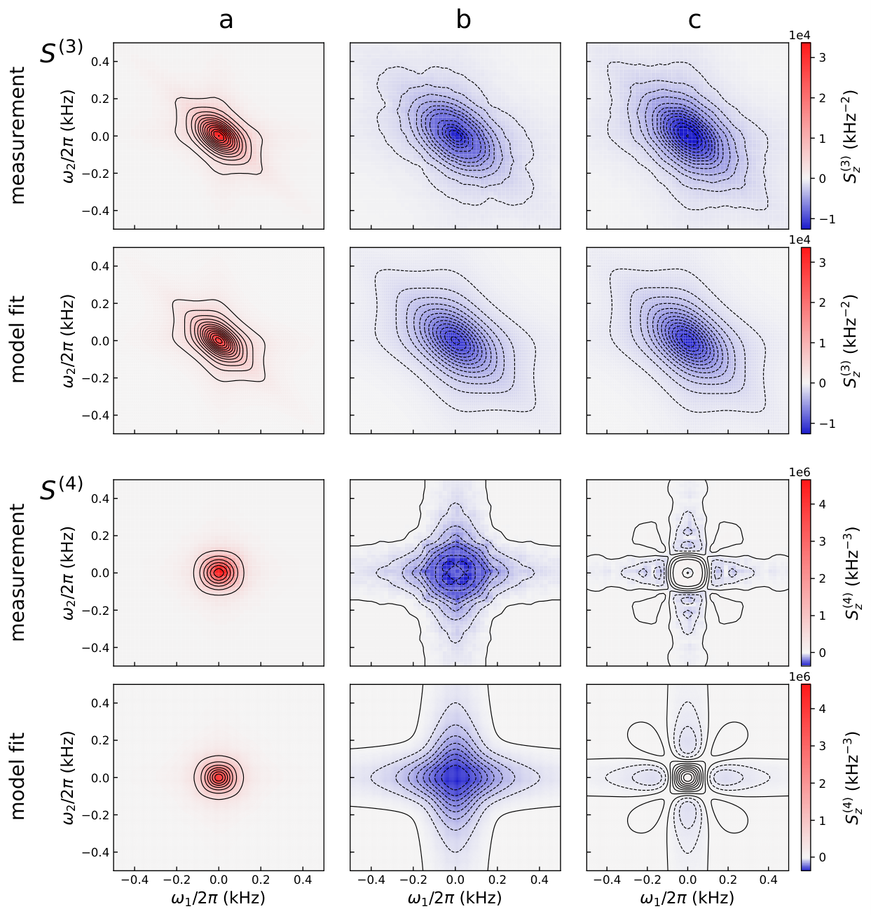
The time traces we are going to model and evaluate were recorded in an experiment by Kurzmann et al. Kurzmann et al. 2019. A single InAs quantum dot within an electrically biased quantum dot layer in a GaAs-based p-i-n diode structure is optically read out via resonance fluorescence (see Fig. 1). The fluorescence time traces exhibit telegraph noise due to the electron occupation dynamics of the quantum dot. The inset of Fig. 2 shows traces for an external magnetic field of 10 T and different gate voltages labeled with a) (360 mV), b) (380 mV), and c) (382 mV). The gate voltages shift the chemical potential of the electron reservoirs with respect to the single-electron level resulting in voltage-dependent tunnel rates. Corresponding power spectra were calculated from time traces of 6 minutes duration each (evaluation scheme see App. B). While the traces clearly show quantitative differences in, e.g., typical up- and down-times, the power spectra are all Lorentzian-shaped and differ only weakly in widths and overall height (see Fig. 2). This changes dramatically for the bispectrum and the fourth-order correlation spectrum (definitions see App. B). Now, clear differences become visible (see Fig. 3): The bispectrum is completely positive for case a) while it is negative for cases b) and c) showing a similar overall structure. Clear differences between cases b) and c) are, however, found in the trispectrum which exhibits a negative peak for case b) but an almost flat negative structure for case c).
In the following, we formulate the SME for the single dot experiment described by Kurzmann. The QD dynamics is modeled by an electron tunneling rate onto the dot and a rate from the dot. Spin-dependent effects can be neglected at high magnetic fields (see below). The quantum states related to the occupied and empty dot follow from each other via a fermionic creation operator and an annihilation operator , respectively. The number operator assumes the eigenvalues 1 and 0, respectively. The SME propagates the density matrix of the quantum dot while it is constantly monitored for its occupation by a continuous measurement given by the operator . This simple model will be extended to a spin-dependent version in Sec. III covering the case of external fields below 10 T. The stochastic master equation (Ito-calculus)
| (1) | |||||
| (2) |
with damping terms
| (3) |
and backaction term
| (4) |
describes the system dynamics and the resulting detector output
| (5) |
as it is monitored for the measurement operator with measurement strength . We use the notation for the measurement strength from Ref. Hägele and Schefczik 2018 and for damping and backaction from Ref. Tilloy 2018. The SME has been derived in various forms and varying generality and was rediscovered several times in literature Barchielli et al. 1982; Barchielli and Gregoratti 2009; Belavkin 1987; Diosi 1988; Gagen et al. 1993; Korotkov 1999; Korotkov 2001; Goan et al. 2001. An especially intuitive way of deriving the SME was given by Gross et al. Gross et al. 2018 and similarly by Atal et al. Attal and Pautrat 2006; Attal and Pellegrini 2010. They introduce a continuous sequence of two-level quantum systems (qubits) that each weakly interact for a short period with the system and are subsequently readout by a projection measurement. The projection measurements give some information on the system and at the same time result in Gaussian background noise as the measurement outcome is still highly stochastic. The interaction with the stream of probe systems also causes measurement-induced system damping. The first line of Eq. (1) is identical to a von-Neumann master equation in Lindblad form which correctly describes incoherent tunneling on and from the quantum dot Lindblad 1976. The Hamiltonian is set to zero since the model here disregards spin dynamics or other coherent behavior. The second line contains the differential of a stochastic Wiener process where with is delta-correlated Gaussian noise. Constant monitoring of occupation leads to overall damping towards an eigenstate of (first term of the second line) and a stochastic measurement backaction on the system which is correlated with the detector output [Eq. (5)] via the common Wiener process. The SME can in principle be solved numerically to simulate time traces (see Fig. 8) which can then be evaluated in terms of polyspectra. Instead, we will use general analytical expressions for the 2nd- to 4th-order multi-time cumulants of for general systems to obtain expressions for higher-order spectra of the quantum dot dynamics Hägele and Schefczik 2018; Hägele et al. 2020. The expressions are given in terms of the system Liouvillian where covers all RHS terms of Eq. (1) but the stochastic backaction term which is non-linear in . We define a system propagator with the Heaviside-stepfunction , a steady state , a measurement operator , and its corresponding super operator not . These definitions allow for a compact notation of multi-time moments Atalaya et al. 2018; Tilloy 2018; Hägele and Schefczik 2018
| (6) |
where time order is required and the system is assumed to be in its steady state . Consequently, the moments depend only on time differences but not on absolute times. Quantum mechanical expressions for multi-time moments in the form of Eq. (6) have been given in the literature before for several special cases. Zoller and Gardiner discuss moments of the photon counting statistics [see Ref. zol 1997, Eq. (98)]. Similarly, already in 1981 Srinivas gives an early theory for photon counting where expressions with very similar structure compared to Eq. (6) appear Srinivas and Davies 1981. Bednorz et al. derive a moment generating functional within a path integral theory assuming a weak measurement limit and evaluate the functional to arrive at Eq. (6) [see Ref. Bednorz et al. 2012, Eq. (17)]. Wang and Clerk find the same functional as Bednorz via a Keldysh approach and use it to calculate ”Keldysh-ordered” moments, cumulants, and spectra of quantum noise up to third order [Ref. Wang and Clerk 2020, Eq. (3)]. Nazarov’s full counting statistics is based on the Keldysh approach and uses a coupled ancilla system to derive a generating functional for moments that yields Keldysh order operators in the Heisenberg picture. The dependence of detector back-action on the measurement strength is however not regarded in that approach Nazarov and Kindermann 2003; Nazarov 2003.
Jordan and coworkers give a path integral framework for treating continuous quantum measurements and apply it to the simultaneous continuous measurement of two non-commuting observables of a single qubit Chantasri et al. 2013; Chantasri and Jordan 2015. They, however, derive ”self-correlators” only up to second order Chantasri et al. 2018. Jordan and coworkers also give an early example of a violation of a generalized Leggett-Garg inequality which is based on second-order moments of weak measurements Jordan et al. 2006; Williams and Jordan 2008. Below we will see that a polyspectrum of at least third order is required to extract tunneling rates from quantum dot measurements. The great advantage of using the SME is that it provides a solid foundation for deriving analytical expressions for higher-order multi-time moments without restrictions on the measurement strength as well as a way to simulate experiment-like time-traces (see Sec. IV).
Cumulants instead of moments are often used in statistics since cumulants of the sum of independent stochastic variables are simply the sum of the individual cumulants. Additive noise in a measurement can therefore be subtracted from cumulant-based quantities. Consequently, the cumulant-based polyspectra are the desired quantities for evaluating quantum noise time traces (App. B). A modified propagator and a modified measurement super operator allow for a compact notation of multi-time cumulants Hägele and Schefczik 2018; Hägele et al. 2020 despite their generally intricate representation in terms of moments (App. A). The expressions
| (7) | |||||
| (8) | |||||
| (9) | |||||
are also valid for equal times and hold without any restrictions on the time order Hägele and Schefczik 2018. The term under the sum yields a contribution if and only if the correct time order for to is fulfilled by one of the permutations. The delta-function in appears due to the Gaussian noise contribution to which is delta-correlated [Eq. (5)]. Unlike moments, cumulants beyond second order are not sensitive to Gaussian noise explaining the absence of delta-functions in and . Compact expressions for cumulants beyond the fourth order are still elusive.
Next, we calculate the multi-time cumulants and quantum polyspectra for the quantum dot model, Eq. (1). The Liouvillian of the quantum dot system can be represented as a matrix with a relatively simple structure acting on the density matrix which itself can be represented by a vector with four entries (compare Section XV of Ref. Hägele and Schefczik 2018). The quantities and can be expressed analytically with the help of computer algebra. Assuming time order , we find the cumulants
| (10) |
| (11) |
| (12) |
where we have introduced the positive time differences . Apart from the -prefactors and the delta-function contribution to , the expressions and agree with those derived from a classical rate equation model Li et al. 2013. The cumulants to show no further dependence on despite the fact that the Liouvillian contains a -dependent damping term. A dependence of cumulants on can be found, e.g., in systems where a large measurement strength leads to suppression of coherent dynamics (Zeno-effect) Misra and Sudarshan 1977; Korotkov 2001. The absence of a -dependence in our system is explained by the absence of coherent dynamics ().
The analytical expressions for the polyspectra follow after Fourier transformation of the cumulants with respect to [Eq. (27)]. In Sec. XIV of Ref. Hägele and Schefczik 2018 it is shown how in general the time order can be dealt with when performing a multi-dimensional Fourier transform. We obtain
| (13) | |||||
| (14) |
A cut through the trispectrum is given in the Appendix, Eq. (41). Alternatively, a direct evaluation of the quantum polyspectra in the frequency domain yields the same results (App. C). Similar to the cumulant expressions, the measurement strength leads for the present system only to a prefactor in the polyspectra and a variation of the spectrally flat background noise in . In contrast, we will treat in Section V a double-dot system where an increasing measurement strength leads to a clear suppression of coherent quantum oscillations and a corresponding overall change in the polyspectra.
The experimental time traces of the quantum dot occupation dynamics are evaluated for and by simultaneously fitting the analytical expression of the spectra , , and to the spectra of the measured time traces. A constant background contribution to the power spectrum is also regarded separately. Time traces of 6 min durations with a temporal resolution of 100 s were taken for each gate voltage. The measured traces and differ by a setup-dependent scaling factor that is regarded in the fitting procedure. In our case, the scaling factor is negative since the occupied quantum dot state results in absent fluorescence.
The polyspectra for cases a), b), and c) obtained from fitting are displayed for illustration along with the originally measured spectra in Fig. 3. The three sample traces of Fig. 2 can now be attributed to three regimes of the tunneling rates: a) , b) , and c) . Figure 4 compares as an important result the tunneling rates for different gate voltages and a magnetic field of 10 T obtained from polyspectra with those obtained from a previous analysis of the waiting-time distribution (WTD), i.e, of the full counting statistics Kurzmann et al. 2019; Kur.

The excellent agreement demonstrates that polyspectra are a powerful tool for evaluating transport measurements. The general weak variation in the power spectra is easily explained by Eq. (13) which does depend only on the sum of the tunnel rates. The prefactor can not be exploited to separate and since the measurement strength acts as an overall scaling parameter. In contrast, the prefactor of the bispectrum, Eq. (14), together with the prefactor of the power spectrum contain information on and are in principle sufficient to extract both parameters. We found more reliable results by simultaneously fitting also the fourth-order spectrum which is sensitive to and [see Eq. (12)]. We note that the second- and fourth-order spectrum do not change under exchange of and making the evaluation of the bispectrum mandatory.
III Spin-dependent quantum dot dynamics
Next, we apply our method to a quantum dot in magnetic fields below 10 T. Following Kurzmann et al. Kurzmann et al. 2019, the Zeeman spin splitting leads to spin-dependent tunneling rates
| (15) |
The tunnel-coupling strength characterizes the tunnel barrier, is the Fermi distribution function of the electron reservoir, the quantum dot level energy is given by , and the temperature by K. The prefactor regards a reduction of the tunneling due to the presence of the exciton whose fluorescence is detected by the measurement setup Kurzmann et al. 2019. After introduction of a spin relaxation rate to the down state, the system is fully described by an incoherent transition dynamics depicted schematically in Fig. 5. Spin flips to the up state are neglected as the spin down state is energetically favorable in magnetic fields Kurzmann et al. 2019.

The model in Kurzmann et al. can be formulated as a stochastic master equation
| (16) | |||||
with detector output
| (17) |
The measurement operator appears as a sum since the detection scheme does not distinguish between up and down spins, but is only sensitive to the mere presence of an electron in the quantum dot.
As an example, the power spectrum, bispectrum, and trispectrum were calculated from Eqs. (38) to (40) for tunneling rates kHz, kHz, and absent spin relaxation (see Fig. 6). Their structure is clearly different from the spectra of the simple quantum dot model discussed above. The power spectrum appears to be a superposition of two Lorentzian peaks. The bispectrum reveals a small dip at zero frequencies and the trispectrum displays positive maxima on the diagonals that were absent for the simple quantum dot model. Spin relaxation rates larger than the tunneling rate cause practically all electrons to tunnel from the QD via the spin-down level at the rate while electrons enter the empty dot at an effective rate . The dot dynamics, therefore, follow the simple quantum dot model and the spectra resume the appearance of spectra shown in Fig. 3. The dependence of the spectra on the spin relaxation rate suggests that the spin relaxation rate can be extracted from data measured at finite magnetic fields. This dependence will get weaker for similar tunneling rates of the two spin orientations, i.e. and . For exact agreement, the occupation dynamics will obviously not depended on the spin orientation and is therefore not sensitive to the spin relaxation rate.
In contrast to the simple model above, analytical expressions for the spectra are not available. The fitting procedure, therefore, relies on a numerical evaluation of the quantum polyspectra via Eqs. (38) to (40). The parameter space for the five relaxation rates is restricted by their dependence on and [compare Eqs. (15)]. Spin relaxation rates were determined for a gate voltage of 371 mV at a field of 2 T and for 376 mV at 4 T. We obtain an almost perfect agreement between data and model for both fits. Fig. 7 shows for a quantitative comparison cuts of all three spectra along the axes and cuts for the bi- and trispectra along their diagonal .
The 2 T-case yields kHz and tunneling rates kHz. For 4 T we obtain kHz and tunneling rates kHz. The discrepancy to the values given in Kurzmann et al. for 2 T kHz and 4 T kHz may be explained by a weak dependence of the tunneling rates on the spin orientation and a large spin relaxation (see previous paragraph). In both cases, the spin-relaxation rate has only little influence on the tunneling dynamics giving rise to large errors in the model fit.

IV Evaluating transport in the weak measurement regime
The experimental time-traces from above exhibit telegraph noise and a small amount of additional noise. This allows in principle for the evaluation of data in terms of waiting-time distributions of the FCS. Continuous measurement theory, however, states that telegraph noise does disappear for weaker measurements. Such a disappearance was recently reported for the case of gate-tunable quantum point contacts Küng et al. 2009. It was shown that a cross-correlation spectrum of two adjacent QPCs showed similar signatures as the spectra from the stronger measurement regime Küng et al. 2010. However, an analysis in terms of the full counting statistics as, e.g., previously required for separating in- from out-tunneling rates is no longer possible for vanishing telegraph behavior. Here we show that an evaluation of general time traces in terms of quantum polyspectra is possible even in the weak measurement regime without any restrictions.
We simulate a weak measurement ( kHz) on a quantum dot, Eq. (1), with parameters = 1 kHz and kHz. The integration of the SME with the QuTiP software package Johansson et al. 2013 yields the QD occupation (see Fig. 8, dark blue curve). It assumes values in the full regime between 0 and 1. Hence, the system is not being projected into one of its eigenstates. The actual detector time trace exhibits large background noise (see Fig. 8, light blue curve) that dramatically exceeds the interval from 0 to 1, an effect put forward by Aharonov et al. in their pioneering work on the notion of weak measurements Aharonov et al. 1988. Quantum jumps can no longer quantitatively be evaluated from the time trace and methods related to the FCS cannot be applied. Fig. 9 (left column) shows polyspectra calculated from the simulated measurement trace with a duration of 30 minutes. The polyspectra follow from a scheme based on multivariate cumulant estimators of Fourier coefficients of the time trace (App. B). We see excellent agreement between numerical spectra and the ones evaluated from the exact expressions for quantum polyspectra, Eqs. (38), (39), and (40). For comparison of spectra, no addition normalization was needed as prefactors arising, e.g., from the spectral window were correctly accounted for by our formulas. The simulated polyspectra exhibit increasing noise for increasing order which is a known feature for estimates of cumulant-based quantities McCullagh 2018. The negative bispectrum immediately reveals . A simultaneous fit of all spectra yields the predefined tunneling rate within an error of 10 %. Traces with even stronger background noise can be evaluated if spectra are averaged for sufficiently long measurement times.

Next, we shortly discuss the nature of the SME detector model in comparison with another model that was recently investigated by Li et al. in the context of a randomly flipping spin Li et al. 2013. The time trace in Figure 8 corresponds to the noisy current that traverses a quantum point contact and thereby probes the quantum dot occupation. In the above case of weak coupling, the probe current modulation due to the dot occupation is much weaker than the omnipresent shot-noise. Nevertheless, cumulants and spectra for order three or higher exhibit only signatures of the quantum system as they are not sensitive to Gaussian shot-noise. Li et al. give a different example of a continuous measurement on a two-level system Li et al. 2013. Their detector model yields a -1 or 1 for the two levels and 0 if no information could be gathered. For a slow telegraph dynamics of the system, the jump dynamics can be resolved in the detector stream and spectra similar to ours [Eqs. (13), (14), and (41)] were recovered. For system dynamics faster than the average appearance rate of 1 or -1 (a weak measurement in the terminology of Li) the authors find by a numerical simulation of the detector output that their fourth-order cumulant “quickly deteriorates” and no longer bears resemblance with the desired spectra. A full theory of their detector model that would be capable of predicting spectra in the spirit of our C1 to C3 for different measurement strength is, however, still elusive. A separation of detector-related and system-related contributions to polyspectra remains therefore as a challenge in the case of Li’s detector model.
V Zeno-transition in a double-dot system
The quantum system treated in the preceding section was completely dominated by incoherent tunneling dynamics and spin relaxation. Consequently, coherent quantum dynamics was neither expected to leave a signature in the experiment nor needed to be described by a Hamiltonian (i.e., so far ).
The SME is, however, capable of describing coherent quantum dynamics and the effect of a continuous measurement on the dynamics. Here, we investigate the transition from the weak to the strong measurement regime in a double-dot system where electrons can coherently oscillate between the dots due to tunnel coupling. The dynamics follows from the hopping term that quantifies the coupling of the dots
| (18) |
where is the coupling constant and () is the annihilation operator acting on the first (second) QD. We neglect the spin degree of the electrons. The stream of electrons between the leads through the system is modeled via incoherent tunneling as presented in Section II. The electrons can enter the system only via the first dot and leave it only via the second dot. The Hamiltonian allows for the simultaneous occupation of both dots with one electron each. A continuous measurement of the occupation of the second quantum dot is modeled by the operator , which corresponds to a measurement via a QPC in the vicinity of the second dot. The SME becomes
| (19) | |||||
with the detector output
| (20) |
The parameters , and are used for the calculation of system dynamics and quantum polyspectra. Fig. 10 shows the transition of the system from the weak measurement regime to the quantum Zeno regime. Each row depicts the occupation dynamics and the quantum polyspectra , , and for increasing measurement strengths [calculated from Eq. (38), (39), (40)]. The transients of the occupation dynamics start at with the first dot fully occupied. In the weak measurement case, the system relaxes towards the steady state where . The weak measurement is however causing non-vanishing oscillations in as the system is forced to reveal partly whether the second dot is empty or full. A subsequent oscillation dynamics towards or from the dot, respectively, needs then to occur. The polyspectra thus reveal a signature at frequency . The occupation number oscillates around a value that itself exhibits slow fluctuations in time. The reason being that the number of electrons in the system is not strictly conserved due to random tunneling events from and into the leads. Consequently, a clear peak at zero frequency appears in all spectra.
For low measurement strength (first and second row), we find sharp spectral lines in , , and . The lines in exhibits the same characteristic butterfly signature as display in Figure 14 of Smirnov et al. smi 2020. For increasing measurement strengths (third and fourth row) the oscillating dynamics become more and more suppressed. Telegraph-like switching is observed for the strongest measurement strength where all coherent dynamics is suppressed (so-called quantum Zeno regime). Consequently, all peaks in the spectra move towards zero frequency. The incomplete switching events seen in transient for the largest measurement strength are known as spikes and have been investigated in detail by Tilloy Tilloy et al. 2015. The white background noise in decreases as the expectation value in Eq. (20) dominates over the Gaussian noise term for large . The signatures in and are equally broadened as signals from a larger range of frequencies are getting correlated. The quantum Zeno effect had been previously studied theoretically by Korotkov in a double-dot system without leads. He found a damping of oscillation dynamics and a correspondingly broadened spectral line in his Korotkov 2001. As a consequence of leads, our exhibits an additional peak at zero frequency (see above). Korotkov finds an unrelated peak at zero frequency only after introducing an energy imbalance of the two dots. Suppression of coherent dynamics was recently observed in experiments on a superconducting qubit in a GHz-cavity (circuit quantum electrodynamics) where measurement strengths and observation operators were highly controllable Ficheux et al. 2018. The dynamics of the system was obtained from averaging many noisy time-traces for an identically prepared initial state, while here steady state fluctuations are observed and analyzed without the need for state preparation. While we are currently not fully able to interpret all features in the higher-order spectra, it is clear that they contain more information than usual power spectra. Our analysis of a real-world experiment in Sections II and III demonstrates that higher-order spectra can contribute substantially to the analysis of quantum systems.
VI conclusion
We presented quantum polyspectra within a stochastic master equation approach as a viable alternative to full counting statistics approaches for evaluating time-traces of transport measurements. The framework is applicable to general systems where both coherent evolution and incoherent coupling to the environment are important Jacobs and Steck 2006. The stochastic master equation has previously been shown to cover the whole regime from weak to strong measurements and allows for modeling of the weak measurement regime as well as investigating the transition to the Zeno regime Korotkov 2001. In quantum electronics, quantum polyspectra can in the future be used for evaluating weak quantum point contact measurements where background noise prevents a traditional analysis in terms of the full counting statistics, i.e. when quantum jumps can no longer be identified from time traces. Weakly coupled QPCs and polyspectra may be the key for fully characterizing coherent dynamics in transport measurements like, e.g., spin precession or tunnel dynamics between adjacent quantum dots Koppens et al. 2006. We also expect applications of quantum polyspectra in circuit quantum electrodynamics and quantum optics in general Norris et al. 2016; Ficheux et al. 2018; Minev et al. 2019; Wang and Clerk 2020.
Acknowledgements.
We acknowledge financial support by the Deutsche Forschungsgemeinschaft (DFG, German Research Foundation) Project No. 278162697— SFB 1242. D. H., M. G., and A.L. acknowledge financial support by the DFG by the individual research grants No. HA3003/7-1, No. GE2141/5-1, and No. LU2051/1-1.Appendix A Cumulants
The cumulants can be represented in terms of products of moments as Mendel 1991; Gardiner 2009
| (21) | |||||
| (22) | |||||
| (23) | |||||
Appendix B Polyspectra and their estimation from time traces
Starting from the auto-correlation function of the detector output
| (24) | |||||
where relates to the ideal infinite time average with respect to , the power spectrum
| (25) |
can be defined. Alternatively, the power spectrum can be expressed via the Fourier transform of the detector output as
| (26) |
Brillinger generalized this expression to define polyspectra of order (Ref. Brillinger 1965)
| (27) | |||||
Above, the bispectrum
| (28) |
and a cut through the trispectrum
| (29) |
are used for characterizing experimental time traces and comparison with quantum polyspectra. Polyspectra are estimated from experimental time traces in the following way: The detector output is discretized and divided into time frames leading to arrays of length with
| (30) |
where is the temporal length of the time frames. The coefficient of the discrete Fourier transformation (fast Fourier transformation can be used for evaluation) are obtained after applying a window function to
| (31) |
Window functions are routinely used in signal processing for improving the spectral resolution Harris 1978. Here we appy the approximated confined Gaussian window with window parameter (Figure 11) for its optimal RMS time-bandwidth product Starosielec and Hägele 2014.
The ideal polyspectra are then approximately (finite spectral resolution) given by Schefczik 2020
| (32) | |||||
| (33) | |||||
| (34) |
where for and for . The cumulants , , and (see App. A) are estimated from so-called cumulant estimators sch 2019
| (35) | |||||
| (36) | |||||
| (37) | |||||
where o.p. means ”other permutations”. The overline denotes an average of samples. Their structure is similar to that of the cumulants apart from -dependent prefactors [compare Eqs. (21)-(23)]. The estimators have the property for finite (unbiased estimators) and for (consistency). The estimators , , and are multivariate versions of the well-known k-statistics Fisher 1928; Kendall 1943; McCullagh 2018; Cook 1951. The estimator is identical with a frequently used estimator for the variance of . It exhibits the typical prefactor which is sometimes called the Bessel-correction Kenney and Keeping 1951.
Appendix C Quantum polyspectra
The polyspectra of detector output of the continuously monitored quantum system in the steady state follow from the SME without any approximations as
| (38) | |||||
| (39) | |||||
| (40) | |||||
Their derivation via multi-time cumulants of and an efficient method for their numerical evaluation are given in Refs. Hägele and Schefczik 2018; Hägele et al. 2020. All spectra are free from delta-function contributions because the time-dependent decays exponentially to zero for increasing as long as existence of a steady state for can be assumed.
Appendix D The fourth-order trispectrum of the SQD
Analytical expression for the trispectrum of the quantum dot system (neglecting spin-dependent dynamics):
| (41) | |||||
References
- Blais et al. (2020) A. Blais, S. A. Girvin, and W. D. Oliver, Quantum information processing and quantum optics with circuit quantum electrodynamics, Nat. Phys. 16, 247 (2020).
- Degen et al. (2017) C. L. Degen, F. Reinhard, and P. Cappellaro, Quantum sensing, Rev. Mod. Phys. 89, 035002 (2017).
- Ubbelohde et al. (2012) N. Ubbelohde, C. Fricke, C. Flindt, F. Hohls, and R. J. Haug, Measurement of finite-frequency current statistics in a single-electron transistor, Nat. Commun. 3, 612 (2012).
- Kurzmann et al. (2019) A. Kurzmann, P. Stegmann, J. Kerski, R. Schott, A. Ludwig, A. D. Wieck, J. König, A. Lorke, and M. Geller, Optical detection of single-electron tunneling into a semiconductor quantum dot, Phys. Rev. Lett. 122, 247403 (2019).
- Levitov et al. (1996) L. S. Levitov, H. Lee, and G. B. Lesovik, Electron counting statistics and coherent states of electric current, J. Math. Phys. 37, 4845 (1996).
- Bagrets and Nazarov (2003) D. A. Bagrets and Y. V. Nazarov, Full counting statistics of charge transfer in Coulomb blockade systems, Phys. Rev. B 67, 085316 (2003).
- Fricke et al. (2007) C. Fricke, F. Hohls, W. Wegscheider, and R. J. Haug, Bimodal counting statistics in single-electron tunneling through a quantum dot, Phys. Rev. B 76, 155307 (2007).
- Belzig (2005) W. Belzig, Full counting statistics of super-Poissonian shot noise in multilevel quantum dots, Phys. Rev. B 71, 161301(R) (2005).
- Sukhorukov et al. (2007) E. V. Sukhorukov, A. N. Jordan, S. Gustavsson, R. Lecturq, T. Ihn, and K. Ensslin, Conditional statistics of electron transport in interacting nanoscale conductors, Nature Phys. 3, 243 (2007).
- Flindt et al. (2009) C. Flindt, C. Fricke, F. Hohls, T. Novotny, K. Netocny, T. Brandes, and R. J. Haug, PNAS 106, 10116 (2009).
- Cook (1981) R. J. Cook, Photon number statistics in resonance fluorescence, Phys. Rev. A 23, 1243 (1981).
- Kambly et al. (2011) D. Kambly, C. Flindt, and M. Büttiker, Factorial cumulants reveal interactions in counting statistics, Phys. Rev. B 83, 075432 (2011).
- Stegmann et al. (2015) P. Stegmann, B. Sothmann, A. Hucht, and J. König, Detection of interactions via generalized factorial cumulants in systems in and out of equilibrium, Phys. Rev. B 92, 155413 (2015).
- Emary et al. (2007) C. Emary, D. Marcos, R. Aguado, and T. Brandes, Frequency-dependent counting statistics in interacting nanoscale conductors, Phys. Rev. B 76, 161404(R) (2007).
- Crooker et al. (2004) S. A. Crooker, D. G. Rickel, A. V. Balatsky, and D. L. Smith, Spectroscopy of spontaneous spin noise as a probe of spin dynamics and magnetic resonance, Nature 431, 49 (2004).
- Oestreich et al. (2005) M. Oestreich, M. Römer, R. J. Haug, and D. Hägele, Spin noise spectroscopy in GaAs, Phys. Rev. Lett. 95, 216603 (2005).
- Dahbashi et al. (2014) R. Dahbashi, J. Hübner, F. Berski, K. Pierz, and M. Oestreich, Optical spin noise of a single hole spin localized in an (InGa)As quantum dot, Phys. Rev. Lett. 112, 156601 (2014).
- Hübner et al. (2014) J. Hübner, F. Berski, R. Dahbashi, and M. Oestreich, The rise of spin noise spectroscopy in semiconductors: From acoustic to GHz frequencies, Phys. Status Solidi B 251, 1824 (2014).
- Braun and König (2007) M. Braun and J. König, Faraday-rotation fluctuation spectroscopy with static and oscillating magnetic fields, Phys. Rev. B 75, 085310 (2007).
- Glazov and Ivchenko (2012) M. M. Glazov and E. L. Ivchenko, Spin noise in quantum dot ensembles, Phys. Rev. B 86, 115308 (2012).
- Sinitsyn and Pershin (2016) N. A. Sinitsyn and Y. V. Pershin, The theory of spin noise spectroscopy: a review, Rep. Prog. Phys. 79, 106501 (2016).
- Bednorz et al. (2012) A. Bednorz, W. Belzig, and A. Nitzan, Nonclassical time correlation functions in continuous quantum measurement, New J. Physics 14, 013009 (2012).
- Küng et al. (2010) B. Küng, S. Gustavsson, T. Choi, I. Shorubalko, O. Pfäffli, F. Hassler, G. Blatter, M. Reinwald, W. Wegscheider, S. Schön, T. Ihn, and K. Ensslin, Measurement back-action in quantum point-contact charge sensing, Entropy 12, 1721 (2010).
- Brillinger (1965) D. R. Brillinger, An Introduction to Polyspectra, The Annals of Mathematical Statistics 36, 1351 (1965).
- Hägele and Schefczik (2018) D. Hägele and F. Schefczik, Higher-order moments, cumulants, and spectra of continuous quantum noise measurements, Phys. Rev. B 98, 205143 (2018).
- Hägele et al. (2020) D. Hägele, M. Sifft, and F. Schefczik, Erratum: Higher-order moments, cumulants, and spectra of continuous quantum noise measurements [Phys. Rev. B 98, 205143 (2018)], Phys. Rev. B 102, 119901(E) (2020).
- Jacobs and Steck (2006) K. Jacobs and D. A. Steck, A straightforward introduction to continuous quantum measurement, Contemp. Phys. 47, 279 (2006).
- Korotkov (1999) A. N. Korotkov, Continuous quantum measurement of a double dot, Phys. Rev. B 60, 5737 (1999).
- Korotkov (2001) A. N. Korotkov, Output spectrum of a detector measuring quantum oscillations, Phys. Rev. B 63, 085312 (2001).
- Barchielli and Gregoratti (2009) A. Barchielli and M. Gregoratti, Quantum Trajectories and Measurements in Continuous Time: The Diffusive Case, Lecture Notes in Physics 782 (Springer, Berlin Heidelberg, 2009).
- zol (1997) (1997), P. Zoller and C.W. Gardiner, Quantum noise in quantum optics: The Stochastic Schrodinger equation, e-Print: quant-ph/9702030.
- Atalaya et al. (2018) J. Atalaya, S. Hacohen-Gourgy, L. S. Martin, I. Siddiqi, and A. N. Korotkov, Multitime correlators in continuous measurement of qubit observables, Phys. Rev. A 97, 020104(R) (2018).
- Tilloy (2018) A. Tilloy, Exact signal correlators in continuous quantum measurements, Phys. Rev. A 98, 010104(R) (2018).
- Wang and Clerk (2020) Y.-X. Wang and A. A. Clerk, Spectral characterization of non-gaussian quantum noise: Keldysh approach and application to photon shot noise, Phys. Rev. Research 2, 033196 (2020).
- Efimov and Shokurov (2001) V. V. Efimov and M. V. Shokurov, Bispectral analysis of geopotential-height anomalies for synoptic-intraseasonal time-scale, Q. J. R. Meteorol. Soc. 127, 1707 (2001).
- Barchielli et al. (1982) A. Barchielli, L. Lanz, and G. M. Prosperi, A model for the macroscopic description and continual observations in quantum mechanics, Nuovo Cimento 72B, 79 (1982).
- Belavkin (1987) V. Belavkin, Non-demolition measurement and control in quantum dynamical systems, in Information Complexity and Control in Quantum Physics, International Centre for Mechanical Sciences, Vol. 294, edited by A. Blaquiere, S. Diner, and G. Lochak (Vienna, 1987) p. 311.
- Diosi (1988) L. Diosi, Continuous quantum measurement and ito formalism, Phys. Lett. A 129, 419 (1988).
- Gagen et al. (1993) M. J. Gagen, H. M. Wiseman, and G. J. Milburn, Continuous position measurements and the quantum Zeno effect, Phys. Rev. A 48, 132 (1993).
- Goan et al. (2001) H.-S. Goan, G. J. Milburn, H. M. Wiseman, and H. B. Sun, Continuous quantum measurement of two coupled quantum dots using a point contact: A quantum trajectory approach, Phys. Rev. B 63, 125326 (2001).
- Gross et al. (2018) J. Gross, C. Caves, G. Milburn, and J. Combes, Qubit models of weak continuous measurements: : Markovian conditional and open-system dynamics, Quantum Science and Technology 3, 024005 (2018).
- Attal and Pautrat (2006) S. Attal and Y. Pautrat, From repeated to continuous quantum interactions, Annales Henri Poincare 7, 59 (2006).
- Attal and Pellegrini (2010) S. Attal and C. Pellegrini, Stochastic master equations in thermal environment, Open Syst. Inf. Dyn. 17, 389 (2010).
- Lindblad (1976) G. Lindblad, On the generators of quantum dynamical semigroups, Commun. Math. Phys. 48, 119 (1976).
- (45) The conjugate transpose of has to be used in case of a non-hermitian measurement operator Tilloy 2018.
- Srinivas and Davies (1981) M. D. Srinivas and E. B. Davies, Photon counting probabilities in quantum optics, Optica Acta 28, 981 (1981).
- Nazarov and Kindermann (2003) Y. N. Nazarov and M. Kindermann, Full counting statistics of a general quantum mechanical variable, Eur. Phys. J. B 35, 413 (2003).
- Nazarov (2003) Y. V. Nazarov, Quantum Noise in Mesoscopic Physics, NATO Science Series II: Mathematics, Physics and Chemistry, 97 (Springer, Netherlands, 2003).
- Chantasri et al. (2013) A. Chantasri, J. Dressel, and A. N. Jordan, Action principle for continuous quantum measurement, Phys. Rev. A 88, 042110 (2013).
- Chantasri and Jordan (2015) A. Chantasri and A. N. Jordan, Stochastic path-integral formalism for continuous quantum measurement, Phys. Rev. A 92, 032125 (2015).
- Chantasri et al. (2018) A. Chantasri, J. Atalaya, S. Hacohen-Gourgy, L. S. Martin, I. Siddiqi, and A. N. Jordan, Simultaneous continuous measurement of noncommuting observables: Quantum state correlations, Phys. Rev. A 97, 012118 (2018).
- Jordan et al. (2006) A. N. Jordan, A. N. Korotkov, and M. Büttiker, Leggett-Garg inequality with a kicked quantum pump, Phys. Rev. Lett. 97, 026805 (2006).
- Williams and Jordan (2008) N. S. Williams and A. N. Jordan, Weak values and the Leggett-Garg inequality in solid-state qubits, Phys. Rev. Lett. 100, 026804 (2008).
- Li et al. (2013) F. Li, A. Saxena, D. Smith, and N. A. Sinitsyn, Higher-order spin noise statistics, New J. Physics 15, 113038 (2013).
- Misra and Sudarshan (1977) B. Misra and E. C. G. Sudarshan, The zeno’s paradox in quantum theory, J. Math. Phys. 18, 756 (1977).
- (56) Supplemental Material of Ref. Kurzmann et al. 2019.
- Küng et al. (2009) B. Küng, O. Pfäffli, S. Gustavsson, T. Ihn, K. Ensslin, M. Reinwald, and W. Wegscheider, Time-resolved charge detection with cross-correlation techniques, Phys. Rev. B 79, 035314 (2009).
- Johansson et al. (2013) J. Johansson, P. Nation, and F. Nori, Qutip 2: A python framework for the dynamics of open quantum systems, Comput. Phys. Commun. 184, 1234 (2013).
- Aharonov et al. (1988) Y. Aharonov, D. Z. Albert, and L. Vaidman, How the result of a measurement of a component of the spin of a spin-1/2 particle can turn out to be 100, Phys. Rev. Lett. 60, 1351 (1988).
- McCullagh (2018) P. McCullagh, Tensor Methods in Statistics, 2nd ed. (Dover Books, 2018).
- smi (2020) (2020), D. S. Smirnov, V. N. Mantsevich, and M. M. Glazov, arXiv:2010.15763 [cond-mat].
- Tilloy et al. (2015) A. Tilloy, M. Bauer, and D. Bernard, Spikes in quantum trajectories, Phys. Rev. A 92, 052111 (2015).
- Ficheux et al. (2018) Q. Ficheux, S. Jezouin, Z. Leghtas, and B. Huard, Dynamics of a qubit while simultaneously monitoring its relaxation and dephasing, Nature Commun. 9, 1926 (2018).
- Koppens et al. (2006) F. H. L. Koppens, C. Buizert, K. J. Tielrooij, I. T. Vink, K. C. Nowack, T. Meunier, L. P. Kouwenhoven, and L. M. K. Vandersypen, Driven coherent oscillations of a single electron spin in a quantum dot, Nature 442, 766 (2006).
- Norris et al. (2016) L. M. Norris, G. A. Paz-Silva, and L. Viola, Qubit noise spectroscopy for non-gaussian dephasing environments, Phys. Rev. Lett. 116, 150503 (2016).
- Minev et al. (2019) Z. K. Minev, S. O. Mundhada, S. Shankar, P. Reinhold, R. Gutierrez-Jauregui, R. J. Schoelkopf, M. M., H. J. Carmichael, and M. H. Devoret, To catch and reverse a quantum jump mid-flight, Nature 570, 200 (2019).
- Mendel (1991) J. M. Mendel, Tutorial on Higher-Order Statistics (Spectra) in Signal Processing and System Theory: Theoretical Results and Some Applications, Proc. IEEE 19, 278 (1991).
- Gardiner (2009) C. Gardiner, Stochastic Methods, 4th ed. (Springer, Berlin Heidelberg, 2009).
- Starosielec and Hägele (2014) S. Starosielec and D. Hägele, Discrete-time windows with minimal RMS bandwidth for given RMS temporal width, Signal Processing (Elsevier) 102, 240 (2014).
- Harris (1978) F. Harris, On the use of windows for harmonic analysis with the discrete fourier transform, Proceedings of the IEEE 66, 51 (1978).
- Schefczik (2020) F. Schefczik, Theorie kontinuierlicher Quantenmessungen höherer Ordnung und Realisierung eines GPU-GHz-Korrelationsspektrometers, doctoral thesis, Ruhr-Universität Bochum, Universitätsbibliothek (2020).
- sch (2019) (2019), F. Schefczik and D. Hägele, arXiv:1904.12154v1 [math.ST].
- Fisher (1928) R. A. Fisher, Moments and product moments of sampling distributions, Proceedings of the London Mathematical Society s2-30, 199 (1928).
- Kendall (1943) M. G. Kendall, The advanced theory of statistics. Vol. 1, 1st ed. (Charles Griffin and Co., London, 1943).
- Cook (1951) M. B. Cook, Bi-variate k-statistics and cumulants of their joint sampling distribution, Biometrika 38, 179 (1951).
- Kenney and Keeping (1951) J. F. Kenney and E. S. Keeping, Mathematics of Statistics: Part two, 2nd ed. (Van Nostrand, Princeton, New Jersey, 1951).