Quantum deep field: data-driven wave function, electron density generation, and atomization energy prediction and extrapolation with machine learning

Quantum chemical simulations, such as Kohn–Sham density functional theory (KS-DFT) calculations have been recently approximated by machine learning (ML) techniques such as kernel methods Rupp et al. 2012; Brockherde et al. 2017; Faber et al. 2017. Very recently, deep neural networks (DNNs) Schütt et al. 2017; Schütt et al. 2018 have been used to successfully predict molecular properties, such as the atomization energy, HOMO, and LUMO, on large-scale datasets. Although this prediction is fast and accurate, there is a problem: a DNN model for KS-DFT must be consistently based on an understanding of the underlying physics and must not only predict the properties but also provide the fundamental quantum characteristics (i.e., the wave function/orbital and electron density) of a molecule. Most existing DNN models, however, cannot provide the electron density because they consider only the atomic coordinates and ignore the molecular field. Furthermore, they are mainly interested in predicting the final output, i.e., the interpolation accuracy of a molecular property within a benchmark dataset, and do not focus on capturing the fundamental characteristics of molecules. This does not lead to learning a physically meaningful model and extrapolation, i.e., prediction for totally unknown molecules in terms of its size and structure that do not appear in the dataset. Extrapolation is important in not only molecular science but also real applications for transferring to other molecules or crystals and predicting their properties Huan et al. 2016; Jain et al. 2013 in materials informatics.

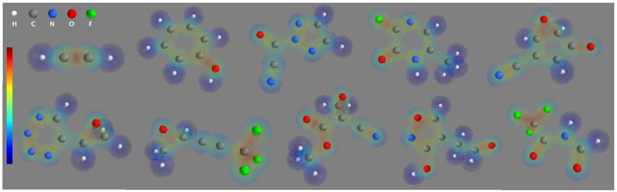
In this letter, we present a simple framework called the quantum deep field (QDF) that provides the electron density of molecules by learning their atomization energies on a large-scale dataset. Crucially, our data-driven QDF framework requires only the molecule–energy pairs (e.g., the QM9 dataset Ramakrishnan et al. 2014) and does not require the molecule–density pairs for training; in other words, QDF generates the electron density indirectly or in an unsupervised fashion with end-to-end physics-informed modeling. The QDF model involves three linear/nonlinear components: (1) a linear combination of atomic orbitals (LCAO): $\phi\rightarrow\psi$, where $\phi$ is the atomic basis function given by the Gaussian-type orbital (GTO) and $\psi$ is the KS molecular orbital, (2) a nonlinear energy functional: $\psi\rightarrow E$, where $E$ is the atomization energy, and (3) a nonlinear Hohenberg–Kohn (HK) map: $\rho\rightarrow V$, where $\rho$ is the electron density and $V$ is the external potential. We optimize all parameters of the LCAO, energy functional, and HK map, in which the latter two are implemented by simple DNNs, simultaneously using the backpropagation and stochastic gradient descent (SGD) Kingma and Ba 2014. We emphasize that learning $\psi\rightarrow\rho\rightarrow V$ serves as the physical constraint on learning $\psi\rightarrow E$ (FIG. 1); this allows QDF to provide valid $\psi$ and $\rho$ (FIG. 2) and leads to high prediction and better extrapolation performance on $E$.

Initially, a molecule is denoted by $\mathcal{M}=\{(a_{1},\mathbf{R}_{1}),(a_{2},\mathbf{R}_{2}),\cdots,(a_{M},\mathbf{R}_{M})\}=\{(a_{m},\mathbf{R}_{m})\}_{m=1}^{M}$, where $a_{m}$ is the $m$th atom, $\mathbf{R}_{m}$ is the 3D coordinate of $a_{m}$, and $M$ is the number of atoms in $\mathcal{M}$. Given $\mathcal{M}$, a set of the molecular orbitals (or wave functions) is denoted by $\{\psi_{1}(\mathbf{r}),\psi_{2}(\mathbf{r}),\cdots,\psi_{N}(\mathbf{r})\}=\{\psi_{n}(\mathbf{r})\}_{n=1}^{N}$, where $\mathbf{r}$ is a position in the field and $N$ is the number of orbitals. The LCAO (or the superposition of wave functions) provides the $n$th molecular orbital:

where $c_{ni}$ is the $i$th coefficient, $\phi_{i}(\mathbf{r}-\mathbf{R}_{i})$ is the $i$th atomic basis function whose origin is $\mathbf{R}_{i}$, and $N$ is the number of basis functions. As the basis function, we use the GTO:

where $D_{i}=||\mathbf{r}-\mathbf{R}_{i}||$, $q_{i}$ is the principle quantum number, $\zeta_{i}$ is the orbital exponent, and $Z(q_{i},\zeta_{i})$ is the normalization term. Additionally, we use the 6-31G basis set and represent $\{\psi_{n}(\mathbf{r})\}_{n=1}^{N}=\bm{\psi}(\mathbf{r})$ with the $N$-dimensional vector:

where $\bm{\psi}(\mathbf{r})\in\mathbb{R}^{N}$ has $\psi_{n}(\mathbf{r})$ as its $n$th element and $\mathbf{c}_{i}\in\mathbb{R}^{N}$ has $c_{ni}$ as its $n$th element. Note that the orbital exponents $\{\zeta_{1},\zeta_{2},\cdots,\zeta_{N}\}=\{\zeta_{i}\}_{i=1}^{N}$ and the coefficient vectors $\{\mathbf{c}_{1},\mathbf{c}_{2},\cdots,\mathbf{c}_{N}\}=\{\mathbf{c}_{i}\}_{i=1}^{N}$ are randomly initialized and then learned/optimized for predicting the atomization energy using the backpropagation and SGD.

For $\bm{\psi}$, we express a DNN-based energy functional $\mathcal{F}_{\text{DNN}}$ as follows:

where $E^{\prime}_{\mathcal{M}}$ is the predicted atomization energy of $\mathcal{M}$. Herein we use a simple feedforward architecture for the implementation of $\mathcal{F}_{\text{DNN}}$, in which the DNN models the interaction between $\psi_{n}$ and $\psi_{m}$. Finally, we minimize the loss function:

where $E_{\mathcal{M}}$ is the atomization energy of $\mathcal{M}$ in the QM9 dataset. Details about $\mathcal{F}_{\text{DNN}}$ and its optimization are described in Supplementary.

Unfortunately, only minimizing $\mathcal{L}_{E}$ does not lead to learning a physically meaningful model; because the DNN has a strong nonlinearity, such a powerful $\mathcal{F}_{\text{DNN}}[\bm{\psi}]$ will output the correct atomization energy $E_{\mathcal{M}}$ even if $\bm{\psi}$ is not valid. In other words, the model does not guarantee the KS orbitals $\bm{\psi}(\mathbf{r})$, which means that $\bm{\psi}(\mathbf{r})$ cannot provide the correct electron density by $\rho(\mathbf{r})=\sum_{n=1}^{N}|\psi_{n}(\mathbf{r})|^{2}$. To address this problem, we impose a constraint on $\bm{\psi}(\mathbf{r})$ based on the HK theorem, which ensures that the external potential $V(\mathbf{r})$ is a unique (i.e., a nonlinear but one-to-one correspondence) function of the electron density $\rho(\mathbf{r})$, i.e., $V(\mathbf{r})\leftrightarrow\rho(\mathbf{r})$. Specifically, we implement the constraint by a nonlinear map $\rho(\mathbf{r})\rightarrow V(\mathbf{r})$, which we refer to as the HK map Brockherde et al. 2017; Moreno et al. 2020 and learn the nonlinearity using a simple DNN.

Formally, we consider a Gaussian external potential Bartók et al. 2010; Brockherde et al. 2017:

where $Z_{m}$ is the nuclear charge of $a_{m}$. We assume $V_{\mathcal{M}}(\mathbf{r})$ to be the correct external potential of $\mathcal{M}$; that is, $V_{\mathcal{M}}(\mathbf{r})$ is used as a target for minimizing loss in the model. Additionally, the electron density is given by

For $\rho(\mathbf{r})$, we express a DNN-based HK map $\mathcal{HK}_{\text{DNN}}$ as follows:

where $V^{\prime}_{\mathcal{M}}(\mathbf{r})$ is the predicted external potential of $\mathcal{M}$. This letter uses a simple feedforward architecture for the implementation of $\mathcal{HK}_{\text{DNN}}$. Finally, we minimize the loss function:

Details about $\mathcal{HK}_{\text{DNN}}$ and its optimization are described in Supplementary.

Note that the HK map used in Brockherde et al. 2017 learns $V(\mathbf{r})\rightarrow\rho(\mathbf{r})$ by a supervised kernel method, where $V(\mathbf{r})$ is the input potential and $\rho(\mathbf{r})$ is the target density to be learned. In contrast, our HK map is different; that is, the direction is opposite, i.e., $\rho(\mathbf{r})\rightarrow V(\mathbf{r})$, where the input density is $\rho(\mathbf{r})=\sum_{n=1}^{N}|\psi_{n}(\mathbf{r})|^{2}$, $\psi_{n}(\mathbf{r})$ is obtained by LCAO, and $V(\mathbf{r})$ is the target potential to be learned.

Furthermore, please note that as a total learning algorithm of QDF, we minimize Eq. (5) and Eq. (9) alternately in an end-to-end fashion and optimize all parameters of the LCAO, $\mathcal{F}_{\text{DNN}}$, and $\mathcal{HK}_{\text{DNN}}$ using the backpropagation and SGD. We believe that this algorithm involving the HK map constraint allows QDF to function as a self-consistent learning machine for KS-DFT.

To evaluate the QDF performance, we first describe the learning/prediction results of atomization energy $E$. For training and testing, we used the QM9under14atoms dataset, which is a subset (15,000 samples of relatively small-sized molecules) of the full set (130,000 samples) of the QM9 dataset (see Supplementary). FIG. 3(a) displays the prediction errors, mean absolute error (MAE, where lower is better) in units of kcal/mol, of our QDF and a baseline model in the form of a learning curve. As the baseline, we implemented a variant of graph neural networks (GNNs) Kearnes et al. 2016, which uses the molecular structure (i.e., the types and 3D coordinates of constituent atoms) alone, does not consider the molecular field, and has hierarchical structure and strong nonlinearity in the modeling phase of the molecular structure. Compared to the GNN, our QDF was able to predict $E$ and its error was much closer to chemical accuracy (1.0 kcal/mol). Additionally, FIG. 3(b) describes how the accuracy improves as the number of training samples increases. The resulting curve was almost linear, and this result is useful for estimating how many training samples are required to achieve a desired accuracy.

TABLE 1 shows the final prediction errors and model sizes of the GNN, QDF, and others Schütt et al. 2017; Schütt et al. 2018 as references. SchNet, which is a variant of the earlier proposed deep tensor neural network (DTNN), is now a standard state-of-the-art deep learning model. We argue that our implemented GNN is not a weak baseline because it achieved a reasonable performance that was competitive with that of DTNN. Additionally, we believe that QDF outperformed (or was competitive with) SchNet in terms of the prediction error; both MAEs were close to 1.20 kcal/mol. In terms of the model size, however, SchNet has more than 1.5 million learning parameters; in contrast, QDF, which has less than half a million parameters, is much more compact.

From the test dataset, we extracted 10 molecules and visualized their electron density maps in FIG. 2 using Mayavi Ramachandran and Varoquaux 2011. We first observed that the electron density $\rho$ is higher at points around C, N, O, and F, which have high electronegativity (red to green) than that at points around H, which has low electronegativity (blue), indicating that $\rho$ transfers from H to C, N, O, and F were qualitatively reproduced by learning the atomization energy $E$. Additionally, $\rho$ increases between two atoms; for example, $\rho$ between two carbon atoms in $\text{C}{\vphantom{\text{X}}}_{\smash[t]{\text{2}}}\text{H}{\vphantom{\text{X}}}_{\smash[t]{\text{2}}}$, $\text{C}{\vphantom{\text{X}}}_{\smash[t]{\text{6}}}\text{H}{\vphantom{\text{X}}}_{\smash[t]{\text{5}}}\text{OH}$, and other molecules are high, indicating that the formation of double and triple bonding was also reproduced. Furthermore, $\rho$ is much higher on the bonding of F atoms. We believe that QDF has the potential to generate valid $\rho$ even if the model is trained only with respect to $E$.

We compared the electron densities obtained by our QDF and a hybrid-functional (B3LYP) simulation, in which we focused on the density profiles along the chemical bonds of ethane ($\text{CH}{\vphantom{\text{X}}}_{\smash[t]{\text{3}}}\text{CH}{\vphantom{\text{X}}}_{\smash[t]{\text{3}}}$) and benzene ($\text{C}{\vphantom{\text{X}}}_{\smash[t]{\text{6}}}\text{H}{\vphantom{\text{X}}}_{\smash[t]{\text{6}}}$) shown in FIG. 4. We first found that the QDF density (red line) could capture the characteristic double peak features of the B3LYP density (yellow dotted line) on the C – C bond in $\text{CH}{\vphantom{\text{X}}}_{\smash[t]{\text{3}}}\text{CH}{\vphantom{\text{X}}}_{\smash[t]{\text{3}}}$ and the C –  – C bond in $\text{C}{\vphantom{\text{X}}}_{\smash[t]{\text{6}}}\text{H}{\vphantom{\text{X}}}_{\smash[t]{\text{6}}}$. Additionally, comparing $\text{CH}{\vphantom{\text{X}}}_{\smash[t]{\text{3}}}\text{CH}{\vphantom{\text{X}}}_{\smash[t]{\text{3}}}$ and $\text{C}{\vphantom{\text{X}}}_{\smash[t]{\text{6}}}\text{H}{\vphantom{\text{X}}}_{\smash[t]{\text{6}}}$, the difference with respect to the sharpness of these double peaks could also be reproduced.

Furthermore, we compared the net charge of an atom in a molecule obtained by our QDF with that obtained by the B3LYP simulation and estimated by Bader analysis Tang et al. 2009. Indeed, Bader analysis cannot be directly applied to the current QDF because we generated the grid points around the atoms assuming a spherical distribution (see FIG. 2 and Supplementary). Therefore, we estimated the net charge of the C atom by summing the electron densities inside a sphere with a specific radius, which is half the length of the C – C bond in $\text{CH}{\vphantom{\text{X}}}_{\smash[t]{\text{3}}}\text{CH}{\vphantom{\text{X}}}_{\smash[t]{\text{3}}}$ (0.76 Å) and the C –  – C bond in $\text{C}{\vphantom{\text{X}}}_{\smash[t]{\text{6}}}\text{H}{\vphantom{\text{X}}}_{\smash[t]{\text{6}}}$ (0.70 Å). Each estimated net charge is as follows: C in $\text{CH}{\vphantom{\text{X}}}_{\smash[t]{\text{3}}}\text{CH}{\vphantom{\text{X}}}_{\smash[t]{\text{3}}}$: 4.05 (B3LYP by Bader), 3.87 (QDF by sphere), and its error is $-4.44\%$; C in $\text{C}{\vphantom{\text{X}}}_{\smash[t]{\text{6}}}\text{H}{\vphantom{\text{X}}}_{\smash[t]{\text{6}}}$: 4.11 (B3LYP by Bader), 3.89 (QDF by sphere), and its error is $-5.35\%$. These indicate that our QDF could quantitatively reproduce the electron density distribution when compared with that calculated by the B3LYP.

Here, note that we simply followed the work of Brockherde et al. Brockherde et al. 2017 and used the Gaussian external potential as a target for learning the HK map. Although the external potential $V$ is not limited to a Gaussian, the current $V$ between two atoms (blue dotted line in FIG. 4) seems to be reasonable for reproducing the double peak of the B3LYP density. We also believe that this Gaussian potential should be improved because our results could not reproduce the density close to the nucleus (green circle in FIG. 4). Hence, another $V$ and atomic orbital, e.g., a Slater-type orbital (STO), would be more suitable. Overall, FIG. 4 demonstrates the viability of QDF for generating valid $\rho$ in an unsupervised fashion.

Lastly, using a more practical evaluation setting, we present evidence that QDF can capture the molecular orbital/wave function and electron density, i.e., the fundamental characteristics of molecules, from a large-scale dataset. We believe that the following result is an interesting finding of this study that has the potential to facilitate extrapolation, which is difficult to solve by general ML approaches in principle.

We assume that if an ML model could capture the fundamental characteristics of data, the model can be used to conduct a prediction for totally unknown data, i.e., perform an extrapolation. This study evaluated an extrapolation as follows: we trained a model with small molecules and then tested it with large molecules. Specifically, we trained the QDF model with small molecules consisting of fewer than 14 atoms (15,000 samples; the prediction performance was already shown in FIG. 3(a) and TABLE 1) and then tested it with large molecules consisting of more than 15 atoms (115,000 samples), which is the remainder of the QM9 dataset (see FIG. 5(a)).

FIG. 5(b) shows the results of this large-scale extrapolation evaluation. The accuracy achieved by GNN is the same as (or superior to) that of the QDF in interpolation; however, the QDF could maintain this accuracy even when the molecular size increases in extrapolation, whereas the GNN could not. Actually, the GNN and its variants have strong nonlinearity in the modeling phase of the molecular structure. By eliminating such nonlinearity using LCAO and imposing the HK map constraint, QDF does not suffer from overfitting. We believe that this is evidence that QDF can capture the fundamental quantum characteristics of molecules that are independent of the system.

FIG. 5(c) shows the error analysis on QDF. We found that the molecules with large errors (over 10 kcal/mol) are often sterically strained or have a cage-like structure and are polarized. However, the number of such molecules in the QM9 dataset is very small, e.g., the ratio of polarized molecules is less than 0.3%. In contrast, although the ratio of molecules including F atom(s) is less than 1.5%, their errors were not large, approximately 0.1 kcal/mol, because these molecules have a stable ring structure and are not polarized; this shows the robustness of QDF.

This study proposed the QDF framework, which is different from other deep learning approaches; in other words, QDF is not an extension of existing DNN models. Our aim was to design a simple DNN model without incorporating complicated techniques/architectures. To model the electron density, some ML approaches have been proposed Grisafi et al. 2018; Zhang et al. 2019; Gong et al. 2019; Chandrasekaran et al. 2019; Ryczko et al. 2019; in particular, we were inspired by Grisafi et al. Grisafi et al. 2018. They (1) created an electron density dataset including 1,000 configurations of a few kinds of small molecules ($\text{C}{\vphantom{\text{X}}}_{\smash[t]{\text{4}}}\text{H}{\vphantom{\text{X}}}_{\smash[t]{\text{6}}}$ and $\text{C}{\vphantom{\text{X}}}_{\smash[t]{\text{4}}}\text{H}{\vphantom{\text{X}}}_{\smash[t]{\text{10}}}$), (2) learned a Gaussian process (GP) model for $\rho$ (i.e., supervised learning) of these molecules, and (3) evaluated the transferability of the learned model by predicting the $\rho$ of large molecules ($\text{C}{\vphantom{\text{X}}}_{\smash[t]{\text{8}}}\text{H}{\vphantom{\text{X}}}_{\smash[t]{\text{10}}}$ and $\text{C}{\vphantom{\text{X}}}_{\smash[t]{\text{8}}}\text{H}{\vphantom{\text{X}}}_{\smash[t]{\text{18}}}$). In contrast, our QDF can be viewed as an unsupervised model to reproduce $\rho$ using only a large-scale dataset of atomization energy $E$ (not $\rho$). Additionally, we demonstrated the large-scale extrapolation in predicting $E$. A supervised model as GP would be relatively easy to train and superior to QDF in predicting $\rho$ because the unsupervised QDF is a model closer to generative adversarial networks Goodfellow et al. 2014 and would be unstable when generating $\rho$.

Furthermore, QDF can also be viewed as one of the approaches such as the physics-informed, Hamiltonian, Fermionic neural networks Raissi et al. 2019; Pun et al. 2019; Greydanus et al. 2019; Pfau et al. 2019; these solve the physical problems and equations using physically meaningful modeling. QDF is designed as a self-consistent machine to solve the KS equation with minimal (three) learning and physical constraint components: LCAO, $\mathcal{F}_{\text{DNN}}[\bm{\psi}]$, and $\mathcal{HK}_{\text{DNN}}(\rho)$. We believe that integrating a supervised model with a dataset of the electron density Sinitskiy and Pande 2018 (i.e., $\rho$ in FIG. 1 is given as a target) and an unsupervised but physically informed and meaningful model with a dataset of the atomization energy, HOMO–LUMO gap, and other properties Chen et al. 2019 will yield an interesting hybrid ML model. QDF will admit many extensions (e.g., for crystals Xie and Grossman 2018) and applications (e.g., for transfer learning to solve more practical problems in materials informatics Huan et al. 2016; Lopez et al. 2016; Kim et al. 2017), and our research position and future directions could prove useful (see Supplementary).

References

- Rupp et al. (2012) M. Rupp, A. Tkatchenko, K.-R. Müller, and O. A. Von Lilienfeld, Physical Review Letters 108, 058301 (2012).
- Brockherde et al. (2017) F. Brockherde, L. Vogt, L. Li, M. E. Tuckerman, K. Burke, and K.-R. Müller, Nature Communications 8, 1 (2017).
- Faber et al. (2017) F. A. Faber, L. Hutchison, B. Huang, J. Gilmer, S. S. Schoenholz, G. E. Dahl, O. Vinyals, S. Kearnes, P. F. Riley, and O. A. Von Lilienfeld, Journal of Chemical Theory and Computation 13, 5255 (2017).
- Schütt et al. (2017) K. T. Schütt, F. Arbabzadah, S. Chmiela, K.-R. Müller, and A. Tkatchenko, Nature Communications 8, 1 (2017).
- Schütt et al. (2018) K. T. Schütt, H. E. Sauceda, P.-J. Kindermans, A. Tkatchenko, and K.-R. Müller, The Journal of Chemical Physics 148, 241722 (2018).
- Huan et al. (2016) T. D. Huan, A. Mannodi-Kanakkithodi, C. Kim, V. Sharma, G. Pilania, and R. Ramprasad, Scientific Data 3, 1 (2016).
- Jain et al. (2013) A. Jain, S. P. Ong, G. Hautier, W. Chen, W. D. Richards, S. Dacek, S. Cholia, D. Gunter, D. Skinner, G. Ceder, et al., APL Materials 1, 011002 (2013).
- Ramakrishnan et al. (2014) R. Ramakrishnan, P. O. Dral, M. Rupp, and O. A. Von Lilienfeld, Scientific Data 1, 140022 (2014).
- Kingma and Ba (2014) D. P. Kingma and J. Ba, arXiv preprint arXiv:1412.6980 (2014).
- Moreno et al. (2020) J. R. Moreno, G. Carleo, and A. Georges, Physical Review Letters 125, 076402 (2020).
- Bartók et al. (2010) A. P. Bartók, M. C. Payne, R. Kondor, and G. Csányi, Physical Review Letters 104, 136403 (2010).
- Kearnes et al. (2016) S. Kearnes, K. McCloskey, M. Berndl, V. Pande, and P. Riley, Journal of Computer-Aided Molecular Design 30, 595 (2016).
- Ramachandran and Varoquaux (2011) P. Ramachandran and G. Varoquaux, Computing in Science & Engineering 13, 40 (2011).
- Tang et al. (2009) W. Tang, E. Sanville, and G. Henkelman, Journal of Physics: Condensed Matter 21, 084204 (2009).
- Grisafi et al. (2018) A. Grisafi, A. Fabrizio, B. Meyer, D. M. Wilkins, C. Corminboeuf, and M. Ceriotti, ACS Central Science 5, 57 (2018).
- Zhang et al. (2019) Y. Zhang, C. Hu, and B. Jiang, The Journal of Physical Chemistry Letters 10, 4962 (2019).
- Gong et al. (2019) S. Gong, T. Xie, T. Zhu, S. Wang, E. R. Fadel, Y. Li, and J. C. Grossman, Physical Review B 100, 184103 (2019).
- Chandrasekaran et al. (2019) A. Chandrasekaran, D. Kamal, R. Batra, C. Kim, L. Chen, and R. Ramprasad, npj Computational Materials 5, 1 (2019).
- Ryczko et al. (2019) K. Ryczko, D. A. Strubbe, and I. Tamblyn, Physical Review A 100, 022512 (2019).
- Goodfellow et al. (2014) I. Goodfellow, J. Pouget-Abadie, M. Mirza, B. Xu, D. Warde-Farley, S. Ozair, A. Courville, and Y. Bengio, in Advances in Neural Information Processing Systems (2014) pp. 2672–2680.
- Raissi et al. (2019) M. Raissi, P. Perdikaris, and G. E. Karniadakis, Journal of Computational Physics 378, 686 (2019).
- Pun et al. (2019) G. P. Pun, R. Batra, R. Ramprasad, and Y. Mishin, Nature Communications 10, 1 (2019).
- Greydanus et al. (2019) S. Greydanus, M. Dzamba, and J. Yosinski, in Advances in Neural Information Processing Systems (2019) pp. 15379–15389.
- Pfau et al. (2019) D. Pfau, J. S. Spencer, A. G. d. G. Matthews, and W. M. C. Foulkes, arXiv preprint arXiv:1909.02487 (2019).
- Sinitskiy and Pande (2018) A. V. Sinitskiy and V. S. Pande, arXiv preprint arXiv:1809.02723 (2018).
- Chen et al. (2019) G. Chen, P. Chen, C.-Y. Hsieh, C.-K. Lee, B. Liao, R. Liao, W. Liu, J. Qiu, Q. Sun, J. Tang, et al., arXiv preprint arXiv:1906.09427 (2019).
- Xie and Grossman (2018) T. Xie and J. C. Grossman, Physical Review Letters 120, 145301 (2018).
- Lopez et al. (2016) S. A. Lopez, E. O. Pyzer-Knapp, G. N. Simm, T. Lutzow, K. Li, L. R. Seress, J. Hachmann, and A. Aspuru-Guzik, Scientific Data 3, 1 (2016).
- Kim et al. (2017) C. Kim, T. D. Huan, S. Krishnan, and R. Ramprasad, Scientific Data 4, 170057 (2017).
Supplementary
Dataset
The QDF model was trained using the QM9 dataset Ramakrishnan et al. 2014, which contains approximately 130,000 samples of small, stable organic molecules made up of H, C, N, O, and F atoms, along with 13 quantum chemical properties (e.g., the atomization energy, HOMO, and LUMO) for each molecule. These molecular properties were obtained by a DFT calculation (Gaussian 09) at the B3LYP/6-31G(2df,p) level of theory. However, the model could not be trained using all 130,000 molecules owing to the computational cost of processing a large number of grid points in each molecular field. Therefore, this study used a subset of the QM9 dataset with a limited number of atoms per molecule, which we refer to as the QM9under14atoms dataset in the main text. The number of samples in the QM9under14atoms dataset was approximately 15,000 molecules. We randomly shuffled and split the QM9under14atoms into training/validation/test sets as 8/1/1, in which the validation set was used to tune the model hyperparameters (see the Hyperparameters section below). We calculated the MAE in TABLE I (in the main text) by taking the mean of all results obtained by 10-fold cross validation (CV) on the QM9under14atoms dataset. Additionally, we chose a result from the CV results and display its learning curve in FIG. 3(a) in the main text. For the extrapolation evaluation, we used the QM9over15atoms dataset (i.e., ), in which the number of samples was approximately 115,000 molecules, which is 10 times more than that of the QM9under14atoms (training) dataset.
We emphasize that since QDF requires only the molecule–energy (or other properties) pairs for training, we can use the popular QM9 dataset. This has the advantage that existing large-scale datasets can be easily leveraged and we could use another one such as the Alchemy dataset Chen et al. 2019. Very recently, a large-scale electron density dataset was created Sinitskiy and Pande 2018 for supervised learning; however, we believe that QDF, which is an unsupervised method for learning electron density, is a reasonable proposition, and integrating the supervised/unsupervised approaches with the density/energy datasets could lead to an interesting hybrid model in the future.
Molecular field definition
Given a molecule , we consider spheres with a radius of Å, where each sphere covers each atom centred on , and then divide the sphere into grids (or meshes) in intervals of Å. This process yields many grid points in , as shown in FIG. 2 in the main text. The grid-based field of is denoted by , where is the 3D coordinate of the th point and is the number of points in .
Architectures of and
To implement described in the main text, given , where each denotes the KS orbitals obtained by LCAO on in the above defined grid field, we first consider the following feedforward architecture: