Law of large numbers for the drift of two-dimensional wreath productThanks: This project has received funding from the European Research Council (ERC) under the European Union’s Horizon 2020 research and innovation program (grant agreement No.725773) The first named author also thanks the support of the ANR grant MALIN
Abstract.
We prove the law of large numbers for the drift of random walks on the two-dimensional lamplighter group, under the assumption that the random walk has finite -moment. This result is in contrast with classical examples of abelian groups, where the displacement after steps, normalised by its mean, does not concentrate, and the limiting distribution of the normalised -step displacement admits a density whose support is . We study further examples of groups, some with random walks satisfying LLN for drift and other examples where such concentration phenomenon does not hold, and study relation of this property with asymptotic geometry of groups.
1. Introduction
In this paper we study the limiting behavior of the distance to the origin of random walks on non-abelian solvable groups, in particular show a law of large numbers type result for random walks of sublinear drift on wreath products over with finite or infinite lamp groups. This is in contrast with classical central limit theorems for random walks on , see e.g., [23, Chapter VIII.4].
Let be a finitely generated group and be a finite generating set of . Denote by the word length function on with respect to the generating set . Let be a probability measure on ; consider a random walk on with step distribution . The drift function is defined as the mean of that is,
If grows linearly, then it is well-known that by Kingman’s subadditive ergodic theorem tends to a positive constant almost surely. If is sublinear, then in general the sequence of normalized random variables does not necessarily converge in distribution. When we say the -random walk is diffusive. In contrast to abelian groups, where symmetric simple random walks have diffusive behavior, there is a rich spectrum of behavior of for symmetric random walks on non-abelian groups: for any subadditive function between and satisfying certain regularity conditions, there exists a group and a symmetric measure on with finite generating support such that is equivalent to , see [2, 10].
In many examples, the limiting distribution of exists and admits a density on . For example, this is the case when is abelian and is a centered measure with finite generating support. This fact can be deduced from the local central limit theorem for random walks on , see e.g. [33, Chapter 2.1].
When converges to a constant almost surely, we say that the distance to the origin of the random walk obeys a law of large numbers. To our knowledge, it has not been studied up to now when such almost sure convergence of to a constant occurs for random walks with sublinear drift function . In this paper, we show a law of large numbers for the displacement of a centered random walk on the wreath product . Recall that the wreath product of groups and is a semi-direct product , where acts by translation on . The group is sometimes called the lamplighter group over (with the lamp group ). We will recall this well-known interpretation as lamplighter in "plan of the proof" section at the end of this introduction.
The study of random walks on wreath products is initiated by Kaimanovich and Vershik, [30], who have shown that wreath products illustrate several phenomena about Poisson boundary on random walks on groups. One and two dimensional wreath products and are examples of groups of exponential growth where the Poisson boundary of simple random walks is trivial; , , are amenable groups with non-trivial boundary of simple random walks; admits (infinite entropy) measures such that the boundary of is non-trivial and the boundary defined by an inverse measure is trivial. The study of Poisson boundary on wreath products was continued in a series of works, among which we mention a recent result of Lyons and Peres, [36], which provide a complete description of the Poisson boundary of simple random walks on , . Many other questions about random walks on wreath products were studied. Here is a non-exhaustive list of problems: return probability on wreath products was studied in papers of Varopoulos [50], Pittet, Saloff-Coste [46] and Revelle [47], Law of iterated logarithm was studied in [48], positive harmonic functions and Martin boundary by Brofferio, Woess [11, 12], minimal growth of (not necessary bounded and not necessary positive) harmonic function by Benjamini et al [5], recurrent subsets (and instability of recurrence of subsets and Green kernel) by Benjamini and Revelle [6]. Our main interest here are infinite wreath products, but we mention that random walks on finite wreath products also provide many interesting examples for the study of random walks on finite graphs, see for instance Häggström and Jonasson [27], Peres, Revelle [43] and Komjáthy, Peres [31] for the study of mixing and relaxation time for random walks on these groups; and Miller, Sousi [38], Dembo et al [18] for the study of late points of random walks. In papers above and in our work, we study Markov kernels invariant by group actions. The work of Lyons, Pemantle and Peres [35] about "homesick" random walks on these groups do not satisfy this condition: a somehow counterintuitive example when inward based random walks move quicker from the origin than simple random walks. Finally, we always discuss here wreath products for the action of the group on itself and we do not mention several recent works about random walks on permutational extensions.
We say that a probability measure on a group is centered if has finite first moment and for any homomorphism . We say that a measure on is non-degenerate if its support generates as a semigroup. The measure has finite -moment if . It is clear that this condition does not depend on the choice of the generating set . Now we formulate our main result for the displacement of random walk on two-dimensional lamplighter groups.
Theorem 1.1.
Let and be a centered non-degenerate probability measure of finite -moment on , . Let be a finite generating set of . Then the -random walk on satisfies
for some positive constant .
We remark that without the second moment condition the normalization can be different from . For instance, there are symmetric random walks with finite first moment on which have linear speed.
We also prove that the law of large numbers for random walk displacement holds in some examples with infinite lamp groups, for instance on the wreath product . In that case the argument relies on a result of Černý [13], see Proposition 5.2. Our main goal is to treat the case where the lamp group is finite as in Theorem 1.1.
Now we comment on the situation in contrast with the phenomenon described in Theorem 1.1. By Gromov’s polynomial growth theorem [25], groups of polynomial growth are virtually nilpotent. In Alexopoulos [1], a local central limit theorem is established for centered finite range random walks on groups of polynomial growth. As a consequence, for centered finite range random walks on polynomial growth groups, converges in distribution and the limiting distribution admits a positive density on the ray Beyond groups of polynomial growth, such convergence in distribution can also be observed in some examples of groups of exponential growth. In Proposition 6.2 we compute the limiting distribution of for symmetric random walks of finite second moment on . Note that in the examples mentioned above, the random walks exhibit diffusive behavior (for an example with non-diffusive drift function where the limiting distribution of can be computed see Example 5.1), it is natural to ask in general the following question.
Question 1.2.
If the random walk on is diffusive, that is is it true that converges in distribution to a limiting law whose density charges the whole ray ?
It is known that the rate of escape of random walks on infinite groups always satisfy a diffusive lower bound, see [34]. In Section 6 we formulate and discuss this question under the stronger assumption that the group admits what is called controlled Følner pairs (see Question 6.1). We provide some evidence supporting a positive answer. As mentioned earlier, Proposition 6.2 describes the limiting distribution of for simple random walks on the lamplighter over with finite lamp group . As another evidence, in Lemma 6.4, we show that if admits a sequence of controlled Følner pairs and limiting density of exists, then the support of the limiting density must be the whole ray The definition of controlled Følner pairs is recalled in Section 6. If instead of a sequence of controlled Følner pairs, we assume a weakened condition that admits controlled Følner pairs on some scales, then the situation is more complicated. We illustrate this by examples of lacunary hyperbolic groups which admit controlled Følner pairs on some scales, where the limiting behavior of depends on the choice of , see Proposition 6.6.
We mention that in certain classes of groups where grows linearly, central limit theorems for are established: see for example the central limit theorem by Benoist and Quint on hyperbolic groups [7]; and more generally on acylindrically hyperbolic groups by a different approach in Mathieu and Sisto [37]. Prior to these works, central limit theorem for the drift of random walk in the Green metric on a hyperbolic group is established by Bjorklund in [8], and for quasimorphisms along random walk trajectories in Bjorklund and Hartnick [9]. In Question 1.2 one might also ask (similar to the situation of abelian groups where the classical central limit theorem holds), whether the limiting density has Gaussian decay at infinity. See more on this in Section 6 and in particular a list of questions after Question 6.1.
Plan of the proof of Theorem 1.1
For simple random walk on , a classical result of Dvoretzky and Erdős [20] shows that the size of the range satisfies the strong law of large numbers:
| (1.1) |
where is the number of vertices visited by the random walk up to time . This result is generalized in Jain and Pruitt [28] where it is shown that for any recurrent random walk on , the strong law of large numbers holds almost surely.
We recall that the name lamplighter for wreath product with the two elements group comes from the following observation. The elements of the wreath product are of the form , where and . One can view the function as a configuration of "lamps", saying that in each element of a base group there is a lamp, which is on if the value is equal to and off if this value is zero, see Figure 1.1 This interpretation is in particular useful when we discuss simple random walks on : the random walker walks on , and at the point he visits he can lit or extinguish the lamp, with some probability specified by the step distribution.

It is well known that the word length in a lamplighter group is closely related to the Travelling Salesman Problem (TSP) in the base group, see e.g. [42]. Therefore it is straightforward that the TSP arises in the study of the drift function of random walks. Basic estimates for the TSP can be useful to understand the behavior of random walks on lamplighter groups, in particular the asymptotics of the drift functions. We also mention that questions in metric geometry, in particular around distortions of embeddings of wreath products into Banach spaces, require deeper understanding of TSP. In Naor and Peres [39], the Jones traveling salesman theorem [29] is applied to construct embeddings of lamplighter groups into Banach spaces.
Denote an element of the lamplighter group by , where and is a function of finite support which we refer to as the lamp configuration of . Consider the standard generating set , where , form the standard basis of , is the constant function on that takes value , and is everywhere in except that it takes value at . Given a finite subset denote by the length of a shortest path in (with respect to the standard generating set ) that visits every point in . One of the usual settings for the TSP also specifies the beginning and ending points of the path. Here we do not specify the beginning and ending points (in the situations we consider the diameter of is much smaller than ). Then the word length of a group element satisfies
where is the cardinality of a set , and .
Consider the standard switch-walk-switch (SWS) measure on , where is uniform on and is uniform on . We refer to the random walk with step distribution as the standard SWS random walk on . Write . Denote by the range of the projected random walk on up to time . It is easy to see that is equivalent to the size of the range , up to a multiplicative constant. Our goal is to determine the asymptotics of when . Given a parameter , the set obtained by keeping each point in independently with probability is called the diluted range with parameter . Then the distribution of of the standard SWS random walk is the same as the diluted range with parameter . Therefore we are led to consider the of the diluted range.
Let be the length of a shortest path that visits the sites of a diluted square two-dimensional lattice of side length with parameter , then by subadditivity, converges to a constant when , see Lemma 2.3. Indeed, the stronger statement that converges to almost surely is true: this observation probably goes back to Beardwood, Halton and Hammersley [4]. The TSP on diluted lattice was considered by Chakrabarti [14] and Dhar et al [19] on the triangular lattice and the square lattice, who estimated the constant in terms of the percolation parameter .
We estimate the length of of the diluted range, claiming that this length, normalised by the size of the range, converges almost surely to a positive constant, see Lemma 2.7. To show this claim we subdivide into boxes of certain side length and inside each each box use the uncrossing Lemma 2.5. Part (i) of Lemma 2.5 is similar the circle freeway lemma used by Lalley in [32] for the TSP of random points on with self-similar distribution; and in part (ii) we estimate the number of "uncrossings". To control the error of approximations, we rely on the Følner property of the range process . Given a finite , denote by the inner boundary of , that is, the set of points in which have at least one neighbor site outside . We say that a sequence of finite sets forms a a Følner sequence if as . Consider the inner boundary of the random walk range . In Okada [40] it is shown that there exists a constant such that . The property that almost surely forms a Følner sequence is proved for a finite range symmetric random walk on in Deligiannidis and Kosloff [17]; and extended to symmetric random walks on with finite second moment in Deligiannidis, Gouëzel and Kosloff [16]. More precisely, by [16, Theorem 12], for a centered, non-degenerate random walk of finite second moment on , there exists a constant such that almost surely
The proof for general random walks as in the statement of Theorem 1.1, not necessarily SWS random walks, follows a similar outline, and we explain below additional arguments we have to use in this general case. We need in particular to have an analog of a "simple" lemma for values of configurations in the wreath product, rather than for diluted squares (see Lemma 3.1); and a more general form of "the Uncrossing Lemma" in terms of wreath products (see Lemma 3.3). We also need to control the closeness of the values of the configuration to the i.i.d. on the range, see Lemma 4.1, in this step we use a result of Flatto [24]. The proof of the main result of that paper is written for simple random walk, but the proof works for centered random walks with -moment, see [24, Remark after Theorem 3.1]. This is the only place we need the finite -moment assumption rather than finite second moment. It is natural to ask whether the statement of [24] is true under finite second moment assumption, but to our knowledge it is not known. Finally, we mention one more extra ingredient what we need for the proof of Theorem 1.1 in the case when the measure is infinitely supported. We need to control large jumps between visited squares of subdivision, see the proof of upper bound for at the end of Section 4 (here the assumption of finite second moment is sufficient).
2. Proof of theorem 1.1 in the case of standard SWS random walk and standard generating set
In this section we consider the case where is the standard generating set of , ; as we have mentioned in the introduction, are standard generators of and is the delta function at , defined by and if . We consider random walk step distribution is the switch-walk-switch measure , where is uniform on and is uniform on . The projection of to is , the standard simple random walk on .
2.1. First observations about range of simple random walks on
Given a finite set , recall that we denote by the length of a shortest path in the Cayley graph of with respect to generators , that visits all vertices in . Note the following property of connected sets in .
Lemma 2.1.
Let be a connected subset of then
Proof.
For any positive integer , subdivide into squares of size . Consider only those squares that intersect with and denote by the union of the perimeters of these squares. Denote by the subset of which consists of points whose squares are not completely contained in . Note that since by assumption is a connected subset of , we have that is connected as well. We have that
Let be a shortest path that goes through all edges in . One can then visit all points in by going along this path through in the following way. We follow the path that visits points of . For each square , look at the first visit of its boundary by . We stop at this point, insert a path that visits all points of , return along to the same point of the boundary of where the path inside is inserted, and then continue along the path . Such path provides an upper bound for
Choosing that such that , we obtain the statement of lemma. ∎
For the -random walk on , by [17, Theorem 4.1], the sequence is almost surely a Følner sequence. Thus we have the following:
Corollary 2.2.
Consider a standard simple random walk on . Let be range of the random walk up to time , then
2.2. An auxiliary fact about TSP on the diluted lattices
Consider a square of size in and denote by the diluted lattice (site percolation) where each vertex of the lattice is present independently with probability . By almost sub-additivity we have the following.
Lemma 2.3.
There exists a constant such that when .
Proof.
We first show the convergence along the subsequence . Consider a square of size and subdivide it into squares , , , .. In each square , , take a traveling salesman path visiting the points in the diluted lattice in . We denote by and the starting and ending point of . Then one can find a path visiting all points in the diluted lattice of the larger square by following the paths and , adding in shortest paths connecting to , to and to . Therefore
Write , then we have that . It follows that the sequence converges to a limit constant . Since , we have that .
For general , take such that . Consider the subsquare of side length inside the square of side length with the same lower left corner. Then we have
| (2.1) |
To get a lower bound, for , divide its sub-square of side length into squares of side length and connecting the TSP inside each small square, we have
| (2.2) |
It follows that converges to as .
∎
Remark 2.4.
2.3. An uncrossing lemma
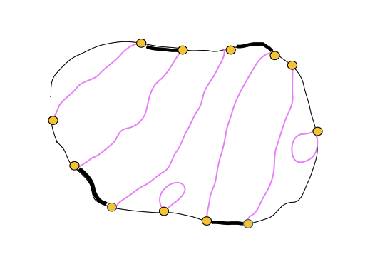
The key ingredient in our argument is the following uncrossing lemma. By a path in we mean a directed path in the standard Cayley graph of . Given a set in and two paths , where each starts and terminates at the boundary , write for the starting point of and for the end point of . We say and have an essential crossing if and are contained in the two different open arcs of between and
Given a finite collection of paths starting and ending at the boundary , we perform the following procedure. If there are two paths and with a common starting/ending point such that , then reversing the direction of one of them if necessary, we replace them by the path which is the concatenation of . By performing this repeatedly, we can replace by in such a way that the starting and ending points of the paths in the new collection are pairwise disjoint. In each starting or ending point appears exactly once, unless there is a path with the same starting/ending point (that is, a loop). Note that by definition, a loop does not have essential crossing with any other path.
Since we consider the standard generating set of , if two paths and have essential crossings then they must intersect. Let be an intersection point of and . We call the following operation uncrossing of and around : replace the path by , where is the concatenation of the segment of from to and the segment of from to ; and similarly replace by which concatenates the segment of from to and the segment of from to . It is clear that the union of images of and is the same as the union of and , and, moreover, and do not have an essential crossing. See Figure 2.1. Note that and might have intersection points other than .

Apply this uncrossing procedure repeatedly, we have the following lemma. The first part is essentially the same as the circle freeway lemma in Lalley [32].
Lemma 2.5 (Uncrossing lemma).
Consider a collection of paths in a finite domain where each path starts and ends on the boundary of .
- (i):
-
There is another collection of paths, which has the same union of their images as the initial one, and no two paths in the new collection has an essential crossing.
- (ii):
-
One can obtain such a collection from the original collection by first replacing by such that the paths in have pairwise disjoint starting and ending points, and then performing at most uncrossings, where is the number of paths in .
Proof.
Given a finite collection of paths in , we first replace by via joining paths (reversing direction of some of them if necessary) as explained before.
We prove the statement by induction on the number of paths of in the collection . Given a path with starting point and ending point , denote by the two arcs on between and . We say that a path in the collection is good if there exists , or , such that all other paths in have starting and ending points in . In particular it implies that has no essential crossings with the other paths. If there is a good path in then we can remove it and apply the induction hypothesis to the collection consisting of the rest of paths. Note that performing uncrossing for the rest of the paths will not introduce any essential crossing with . If there is no good path, pick any path and on the arc take the point which is the closest to which is starting or ending point some other path in the collection. Reverse the direction of if necessary, we uncross and such that one of the new path starts at and end at . Now this new path is good, we remove it and apply the induction hypothesis.
∎
After performing uncrossings to the original collection , we can join the paths in the new collection .
Lemma 2.6.
Suppose is a collection of paths in the domain such that each path starts and ends on and there is no essential crossings between paths of . Then there is a path of total length at most whose image is obtained from the union of paths in by adding connecting segments along the perimeter of .
Proof.
First we pass through all paths that are not loops (see Figure 2.2). The length of this path is at most the sum of the lengths of non-loop paths plus . Then we go through all the loops, passing through any point of the perimeter at most once. It is clear that the total sum of the segments of the perimeter we passed through is at most the length of the perimeter. Therefore the total length of our path is at most sum of the lengths of initial paths plus .
∎
The multiplicative constant in front of is not important for our applications, but it is optimal in the setting of Lemma 2.6.
2.4. Standard random walk on
Denote by the diluted range with parameter . Recall that denotes the shortest length of a path visiting all points in the diluted range . By using the Uncrossing Lemma 2.5, we show that converges to a positive constant almost surely. The steps in the proof are illustrated in Figures 2.3, 2.4 and 2.5.

Lemma 2.7.


Proof.
Take a large integer and divide into boxes of side length . Consider those boxes with non-empty intersection with the range .
We first show an upper bound on by describing a path that visits all points in . Take a path that consists of the union of the perimeters of the boxes with non-empty intersection with . We say a box is fully visited if . Suppose is a box not full, we take a path that starts at a point of , visits all points of and returns to its staring point. The length of such path is at most . If a box is full, then inside we are in the situation of TSP of a diluted lattice. Therefore, to visit all points in , we can go along the perimeter , and in each box we take a shortest path visiting all points inside then return to . The length of such a path is bounded by
| (2.3) |
If a box is not full, then it must contain some point in . Therefore the number of boxes which are not full is bounded by and
Similarly the length of the perimeter union is bounded by
Plugging these bounds into (2.3), we obtain
| (2.4) |
The main contribution to the length of the path comes from the TSP paths in full boxes. Denote by the diluted lattice obtained from a square where each vertex of the square is present independently with probability . By the law of large numbers,
| (2.5) |
Now we turn to the lower bound. Take a global TSP path in the standard generating set of which visits all the points in the diluted range . Consider a box that is fully visited and restrict the path to . We obtain a collection of connected paths where each path starts and ends on the boundary of . We now apply the Uncrossing Lemma 2.5 to this collection of paths and connect the uncrossed paths along the perimeter of , using Lemma 2.6. It follows that there is a connected path of length at most which visits all points in . Therefore, we have that for each fully visited box ,
Summing up over all fully visited box, we have
| (2.6) |
Finally we combine the upper and lower bounds. Given any , by Lemma 2.3, we can take a constant sufficiently large such that
Then by combining (2.4), (2.5) and (2.6) and applying the result that forms a Følner sequence almost surely, we conclude that almost surely,
Since is arbitrary, we have proved the statement.
∎
Proof of Theorem 1.1 for standard SWS measure and standard generating set.
Recall that denotes a -random walk on and we write . The distribution of support of is the same as the diluted range with parameter . For the group element , a path in that connects to satisfies that its projection to the base visits all the points in and in the end arrives at ; and along the way switch on the lamps in . Therefore, we have that
Recall that can be identified with . Since almost surely when , by Lemma 2.7 and the Dvoretzky-Erdös law of large numbers for the range (1.1), we have
∎
3. Uncrossing lemma for wreath product and general generating set
In this section we consider an arbitrary finite generating set of . By an -path we mean a path in the right Cayley graph of , denote by where each and . Recall that an element in the wreath product is denoted by , where and is a function of finite support. Since the lamp group is , the configuration can be identified with the support of , that is, the finite set where the value of is . Given a finite set in , consider an -path in such that is of the form and the support of the lamp configuration of is exactly . Denote by the length of the shortest -path with this property.
Analogous to Lemma 2.3, we have the following convergence of expectation of length of traveling salesman -paths after scaling for the diluted lattice in a square of side length . Consider a square of size in with the lower left corner at . Take the diluted lattice with parameter inside the square where each vertex of the lattice is present independently with probability .
Lemma 3.1.
There exists a constant such that when .
Proof.
Write . For a square of size , subdivide it into squares. In each sub-square , take a shortest -path where the end point of is such that is exactly the diluted lattice in . Write for the starting point of . Then one can find an -path visiting all points in the diluted lattice of the original square by following the paths and , joining their starting/ending points by the shortest -paths connecting to , to and to . Therefore
where the constant only depends on . Write , then . In particular, the sequence is almost monotone and therefore converges to a limit . Since , we have that . To extend the convergence to general , we argue in the same way to establish bounds of the form (2.1) and (2.2) as in Lemma 2.3.
∎
Given an -path , denote by the difference between lamp configurations of and , that is, . Write for the length of the path . Given a collection of -paths, we refer to the sum of configurations as the lamp configuration produced by .
Remark 3.2.
The fact that the lamp group is allows us to reverse the direction of paths. If we reverse the direction of to the path , then the path makes the same changes in the lamp configuration as , while in the projection to the starting and ending points are swapped. This is only valid when the lamp group is .
Next we explain how to perform uncrossings to -paths. Recall that in Section 2 we have defined essential crossings for standard paths in . The notion can be extended to -paths. Two -paths are said to have essential crossings if their projections to have essential crossings. We say two -paths and have an essential crossing in , where starts at and ends at , if , and and are contained in the two different open arcs of between and Here denotes the boundary of with respect to the standard generating set .
The following lemma is a generalization of the uncrossing Lemma 2.5 to -paths. Consider a configuration with . Recall that for the standard generating set considered in Section 2, the length of the shortest path that turns on the prescribed configuration , whose starting and ending point in are and respectively, is exactly the length of a traveling salesman path which starts at , visits every point in , and ends at , plus . And for the standard SWS random walk considered in Section 2, the configuration at time is the diluted range with parameter . Now in the general case (as in the setting of Lemma 3.3 below) we need to control the shortest path to produce the configuration, where possible moves are associated to the generating set (that is, using -paths). For example, these moves can be of the following form: first jump on at distance on the right, turn on the lamp at distance above the marker on and then jump at distance down. Any finite generating set can be interpreted as such rules, with finitely many jumps and finitely many turnings on the lamps. Therefore the following lemma is formulated in terms of wreath products (since it uses -paths) and gives the statement similar to Lemma 2.5 for an arbitrary generating set.
Lemma 3.3 (Uncrossing lemma in terms of wreath product generators).
Let be an square in . Consider a collection of -paths where the projection of each path to starts and terminates on the boundary of . Then one can find another collection of -paths such that there are no essential crossings between paths in , each path in starts and terminates at , and produces the same lamp configuration as . Moreover the total length of -paths in is bounded by
where is a constant only depending on .
Proof.
Given an -path , where each increment , connect each pair by a shortest path in the standard generating set . Denote by the new path in the standard generating set. Given two -paths and in a domain , where starts at and ends at , we perform un uncrossing as follows. First take the paths and in the standard generating set described above associated with and . If and have essential crossings, then we take an intersection point and perform the uncrossing around as described in Subsection 2.3. This way we obtain two paths without essential crossing: which is the concatenation of the sub-path of from to and the sub-path of from to ; and which is the concatenation of the sub-path of from to and the sub-path of from to . Now we convert the paths in the standard generating set back to -paths. If lies on both and , then let be the concatenation of the sub-path of from to and the sub-path of from to ; and similarly for If is not on then let be the closest point to which belongs to the intersection of and the sub-path of from to . Similarly, let the closest point to which belongs to the intersection of and the sub-path of from to . Connect to by an -path of shortest length. Then we define to be the concatenation of the -path from to along , the -path connecting to and the -path from to along . In the same manner we obtain an -path from to .
By the description above, it is clear that and moreover
where the additive constant only depends on the generating set .
Consider a finite collection of -paths whose projection to starts and ends at . If there are two paths and such that , then reversing the direction of one of them if necessary (this is allowed because the lamp group is see Remark 3.2), we replace them by the path which is the concatenation of . By performing this repeatedly, we can replace by such that the starting/ending points of the paths are pairwise disjoint. By the inductive argument in the proof of Lemma 2.5 (ii), the number of uncrossings we need to perform is bounded by . Since each uncrossing costs at most an additive constant , this implies the statement of the lemma.
∎
4. The general case and proof of Theorem 1.1
Throughout this section, let be a symmetric non-degenerate probability measure on with finite second moment; and be a finite generating set of . By raising to a convolution power if necessary, we may assume that and , where . Recall that denotes the word length with respect to the generating set . Recall that one of the assumptions of Theorem 1.1 is that has -moment for some
Let be the projection . Denote by the projection of to . Recall that is a random walk with step distribution on and we write , where is the projection to and is the lamp configuration of Under our assumptions, by [16, Theorem 12], the range process of the -random walk on forms a sequence of Følner sets almost surely: more precisely, there exists a constant such that
We proceed by subdividing the -lattice into boxes of side length , where is an integer depending on (to be specified later). We say a -box is visited up to time instant if is . Note that in a box where every point has been visited by the -random walk up to time , the distribution of the lamp configuration in is in general not uniform on . Instead we use that if the box is visited enough times, then the distribution of the lamp configuration is close to uniform and the TSP of the configuration can be controlled. For this purpose we need the following two lemmas.
Write and , where is the uniform measure on . Let be a sequence of i.i.d. Bernoulli random variables, with and . Let be a sequence of a sequence of i.i.d. random variables with distribution and be a sequence of i.i.d. random variables with distribution . Then
has distribution . We think of the -random walk increments sampled in this way. Write . We say that a location receives a good multiplication up to time instant if there is a time such that and .
By deleting the steps with in the sequence we obtain a sequence of i.i.d. random variables with distribution . Denote by the random walk on associated with this sequence of increments. We say a box is -fully visited by the -walk by the time if for every ,
Denote by the event that the box is -fully visited by the -walk up to time instant .
Lemma 4.1.
Given a box , denote by the set of vertices in which did not have any good multiplication up to time . For any , there exists constants depending only on and , such that
Proof.
Let be an i.i.d. sequence of random variables with distribution , for , independent of the -random walk . Write . Denote by the event that . By the Chernoff bound we have that for some constant that only depends on .
If the box is -fully visited by the -walk by the time , then at time for the walk , the probability that a vertex has not received a good multiplication is bounded from above by
Therefore by the Chernoff bound, we have
∎
Given two configurations in the box , denote by the Hamming distance between them, that is, .
Note that if a site has received a good update before time , then the lamp configuration at is uniform on at time ; moreover the configurations at such sites are independent. The coupling is defined as: takes the same value as at a point in which receives a good update before ; and at a point that does not receive a good update before time , the value of is independent uniform on . Then by definitions we have , where is the set of vertices in which has not received a good update up to time as in Lemma 4.1.
To control TSP of the configuration, we need the following classical bound due to Bartholdi and Platzman [3] (which they prove by space-filling curves heuristics; similar multiscale bound for TSP works for general graphs other than , see e.g., the inequality (17) in [39]).
Lemma 4.2 (Bartholdi-Platzman [3]).
Let be a set of points in a square of side length in . Then .
The rest of this section is devoted to the proof of Theorem 1.1.
Proof of Theorem 1.1.
Recall that we write and , where is the uniform measure on . For any , take sufficiently large such that .
Divide by boxes of side length . We first apply the result from [16] that almost surely forms a Følner sequence, and Flatto’s result in [24] to show that among the visited boxes, the majority of them are -fully visited by the -walk. More precisely, by [24], we have that
where is the number of points visited at least once and at most times by the random walk up to time . Note that the results in [24] is proven for simple random walk on , but the proof applies to any centered random walk on with finite -moment, see the Remark after [24, Theorem 3.1]. If a visited box is not -fully visited, then it must contain a point of . Therefore the number of visited boxes that are not -fully visited is bounded by +.
In a box that is -fully visited by the -walk up to time , consider the restriction of lamp configuration to . Recall that denotes the set of vertices in without good update up to time . As in Lemma 4.1, the configuration can be written as , where the distribution of is uniform on and is a random configuration with support on the set . It follows that to write the configuration one can first write , then correct it by which is supported on , a subset of small size.
To prove the statement, we show that typically is approximated by the contribution from -fully visited box with error bounded by .
The upper bound for : we exhibit an -path that connects the identity to . Recall that we have divided into boxes of side length . Consider all visited boxes and denote by the union of the perimeters of the visited boxes. Because the step distribution allows long range jumps, the union of the perimeters of the visited boxes are not necessarily connected. We add paths to make the union of the perimeters connected. Note that it is sufficient to add connecting paths with total length bounded by the sum of random walk jumps longer than . Indeed, we may enumerate the visited boxes according to the order they are visited as : is the first box visited by the -random walk after that is different from the previous boxes. If the box is not connected to , then we consider the random walk step that first enters and take a shortest path connected the starting and ending point of this step. The union of such additional paths makes the union of the visited boxes connected and the length of the additional paths is bounded by
Take first an -path that starts at identity and covers the perimeters of each visited box, where connecting paths are added according to the long jumps of the random walk as described above. To connect to by an -path, along this path in each box , we take the TSP of the configuration which starts and ends on the perimeter of . Then we can bound the length of the path by
| (4.1) |
where is a constant that only depends on the generating set . Now we choose appropriate such that the main contribution to the quantity on the righthand side of (4.1) is from . To this end, we need the expectation of to satisfy
| (4.2) |
and at the same time to be not too large so that the main contribution still comes from fully visited boxes. More precisely, we need to satisfy both the equation (4.2) above and
Since is assumed to have finite second moment, we have that as . Thus we can choose to be
| (4.3) |
The lower bound for : given an -path connecting to , we consider its restriction to each -full box and use the uncrossing lemma 3.3 to show that the restriction can be modified to provide paths that write the configuration in . The restriction of an -path to means the steps of the path with at least one of whose starting and ending points in . When the path is restricted to a box , we obtain a collection of paths, each with projection to starting and ending near the boundary of . More precisely, there is a constant which only depends on the generating set , such that the starting and ending points of the paths in are within distance to the boundary of . Reversing the directions of some paths if necessary, by concatenating paths we may assume that in the collection , two distinct paths do not share common starting/ending points. In particular, the number of paths in the collection is bounded by , where is a constant only depending on . For each path with starting point and ending point , let ( resp.) be the point on the boundary of closest to ( resp.). Replace by the path which is the concatenation of the shortest -path from to , the path and the shortest path to . Note that . Denote by the collection of modified paths obtained from . The purpose of making such modifications is to assure that paths in the collection start and terminate on the boundary of . Applying the uncrossing Lemma 3.3 to the collection , we obtain a new collection of paths without essential crossings, such that produces the lamp configuration as ; and moreover the total length of paths in is bounded by
where and are constants only depending on the generating set . Reversing the direction of some paths in if necessary (this is allowed because the lamp group is , see Remark 3.2), we can connect the paths in along the perimeter of . This way we produce an -path which produces the configuration , and the length of this path is bounded from above by . To produce the configuration , we continue with a path which writes the difference . Summing over the -full boxes, we obtain the lower bound
| (4.4) |
End of the proof: with the bounds (4.1) and (4.4), the choice of as in (4.3), it suffices to show that a.s.,
By the law of large numbers of arrays of independent random variables to and , the first limit follows from Lemma 3.1 and the second limit follows from Lemma 4.1 and Lemma 4.2.
∎
Remark 4.3.
The only place where we use the -moment condition in the proof is in Flatto’s result [24]. Recall that denotes the number of points visited at least once and at most times by the random walk on up to time . We have shown that if we have a centered non-degenerate probability measure of finite second moment on , such that its projection to satisfies that for any ,
then the statement of Theorem 1.1 would be true for .
Remark 4.4.
For wreath product where is an arbitrary non-trivial finite group, we say that a generating set is complete, if for any , the element is also in the generating set . When , the completeness of a generating set is equivalent to symmetry of . The proof of Theorem 1.1 extends to symmetric non-degenerate random walks of finite -moment on , when the length function is associated with a complete generating set .
Remark 4.5.
When the generating set of the wreath product is not complete, there are configurations where one cannot replace an -path by an -path of comparable length reversing the starting and ending points on . For example, take and the generating set which consists of , and their inverses. In a box of side length , consider the lamp configuration which is on one vertical line and everywhere else, see Figure 4.1. Then for such a configuration, the optimal -path whose projection to travels from bottom to top (red to blue in the picture) is of length ; while the optimal -path which travels from bottom to top is of length at least .

5. Wreath products with infinite lamp groups
In this section we discuss some examples of wreath products with infinite lamp groups. Consider the wreath product , where both and are infinite. Let be a generating set of and a generating set of . We equip with the generating set , where is the function that takes value at and otherwise. Denote by the word length on with respect to the generating set .
Assume that is or and is a finitely generated infinite group. Take a symmetric nondegenerate probability measure of finite support on and a symmetric nondegenerate probability measure on . On the wreath product , take the switch-walk-switch distribution In addition we assume that the drift of the -random walk on with respect to word length has finite second moment and satisfies
| (5.1) |
for some constants and .
With respect to the generating set we have for a group element ,
| (5.2) |
Let be a random walk on with step distribution and write . Since the lamp group is assumed to be infinite and the rate of escape of the -random walk on satisfies (5.2), the length estimate (5.2) shows that the main contribution to is from . Denote by a collection of independent -random walks, indexed by Let be the number of visits to by the projected random walk on the base. Then has the same distribution as . In particular, conditioned on the local times , the random variables , , are independent. Write and . Then by the law of large numbers for independent random variables, we have almost surely
| (5.3) |
where is the limit of , as assumed in (5.1). The problem is reduced to the expression of local times on the base.
For example, when and is a symmetric nondegenerate probability measure on with finite second moment, then the assumption (5.2) is satisfied with and the variance satisfies .
Now we consider an example with as a base group.
Example 5.1.
Let and . Take the probability measure on to be uniform on and take on to be uniform on . On consider the random walk with the standard SWS step distribution . Then by the invariance principle for local times of simple random walk on due to Perkins [45], we have that
where is the local time of the standard Brownian motion.
Next we return to the case of as a base group. Compared to Theorem 1.1, it is easier to establish the law of large numbers for random walks on the wreath product over with an infinite group as lamps. For a switch-walk-switch random walk on , the problem is reduced to functionals of local times on , where a result of Černý [13] can be applied.
Example 5.2.
Let and . Let be a random walk on with switch-walk-switch step distribution , where is uniform on and is uniform on . Then there exists a constant
6. Controlled Følner pairs and limiting behavior of
In general does not necessarily converge in distribution. A strong opposite of concentration of around its mean is that converges in distribution, and the limiting distribution admits a density which is supported on the whole ray . In this section we consider the class of groups which admits controlled Følner pairs.
6.1. Questions
Følner pairs were introduced in Coulhon, Grigoryan and Pittet [15] to produce lower bounds on return probability. We recall the definition: a sequence of pairs of finite subsets of with is called a sequence of Følner pairs adapted to an increasing function if there is a constant and such that for all , we have
- (i):
-
,
- (ii):
-
,
- (iii):
-
.
Følner pairs provide lower bound for return probability for a symmetric probability measure of finite support on , see [15]. The definition of controlled Følner pairs was introduced by Tessera in [49]. We say with is a sequence of controlled Følner pairs if they satisfy (i) and (ii) as above, and
- (iii’):
-
.
Note that it follows from definition that controlled Følner pairs are adapted to the volume growth function of the group.
We ask the following question and in this section provide some evidence supporting a positive answer.
Question 6.1.
Is it true that admitting controlled Følner pairs implies convergence of in distribution and the limiting distribution admits a positive density on ?
In the context of the question, we mention the following asymptotic properties of finitely generated groups.
- 1.
The Følner function is equivalent to the growth function .
- 2.
The group admits a sequence of Følner pairs with volume of equivalent to the growth function .
- 3.
The group admits controlled Følner pairs.
- 4.
The return probability of simple random walk to the origin is equivalent to the solution of
- 5.
Simple random walk on the group has diffusive rate of escape, that is, .
- 6.
Simple random walk on the group is cautious (we will recall the definition of cautiousness in Subsection 6.3).
- 7.
The rate of escape is diffusive and the distribution of converges in distribution to a limiting density whose support is .
So far there is no known example that satisfies one of the conditions in the list but not all the others. All known examples satisfying these conditions are elementary amenable, in particular, there is no known example of group of intermediate growth with properties in the list. One can also ask when the rate of escape is diffusive, whether the entropy of the random walk is equivalent to . Another question one can ask in the setting of condition 7 is whether exhibits Gaussian tail decay, that is, there exists a constant such that
We remark that properties in the list 1-6 describe some asymptotic properties of the group that are minimal possible. Recall that by [34], the rate of escape of simple random walk on an infinite group has a diffusive lower bound. Property in the list describes that the rate of escape is minimal possible in the sense that it is equivalent to the universal lower bound. By the Coulhon-Saloff-Coste inequality, the Følner function is at least the volume growth. For example, on a group of exponential volume growth, the Coulhon-Saloff-Coste inequality implies that the Følner function is at least exponential and the return probability satisfies . Property 1 and 4 describe that the Følner function (return probability of simple random walk resp.) is minimal (maximal resp.) possible given the volume growth. Properties 2 and 3 are strengthenings of Property 1, concerning not only the cardinalities of Følner sets, but also the shape and geometry of them.
One class of groups where the positive answer to Question 6.1 is known consists of groups of polynomial growth. Note that groups of polynomial growth admit controlled Følner pairs. As already mentioned in the Introduction, on groups of polynomial growth, one can apply the local limit theorem in Alexopoulos [1]. More precisely, let be a group of polynomial growth and be a symmetric probability on with finite generating support. Then [1, Corollary 1.19] states that for any , there is a constant such that
where is the limiting Laplacian on a nilpotent Lie group which is referred to as the stratified Lie group associated to in [1]. The stratified nilpotent group admits a dilation and the transition probabilities of the limiting process is scale invariant with respect to the dilation: . The local limit theorem implies that converges in distribution and the limiting distribution admits a positive density on .
6.2. The example of
In this subsection we explain the case of the lamplighter over with the lamp group a finite nontrivial group. The group is an example of a group of exponential growth that admits controlled Følner pairs. We show that for simple random walk on , the limiting distribution of satisfies the claim of Question 6.1. Let be the standard Brownian motion and denote by the size of the range of the standard Brownian motion at time .
Proposition 6.2.
Let be a non-degenerate symmetric measure of finite second moment on , is a finite group, . Let be a finite symmetric generating set of . Then there exists constants such that converges in distribution to , where is the variance of .
Proof.
We first explain a particular case which is easier. Consider the SWS generating set which consists of elements of the form , where , and their inverses. Take the random walk step distribution to be uniform on . Recall that for an element , for the SWS generating set , we have
if . Denote by the range of the projected -random walk on at time . Then there is a constant , almost surely for all sufficiently large,
| (6.1) |
In [28], a central limit theorem for is shown: converges to in distribution. This follows from Donsker’s invariance principle, and similarly one can show that converges to in distribution. Denote by the density of the random variable . Thus by (6.1), we have that the limiting density of is .
Next we consider the general case. We argue in a way similar to the proof of Theorem 1.1, except that in the one-dimensional case the uncrossing lemma is not needed. Note the following consequence of sub-additivity.
Lemma 6.3.
Let be a configuration uniform on . Denote by the shortest -path that writes whose projection in starts at and ends at . Then there are constants such that almost surely
Proof.
[Proof of Lemma 6.3]
Let be the i.i.d. uniform configuration on Given two integers , denote by the restriction of to the interval . Then there is a constant which depends only on such that for any , we have
| (6.2) |
Indeed if we have paths of optimal length starting and ending at producing , and of optimal length starting and ending at y producing , then we may obtain the following path which writes . Follow , which starts at , until the first time it exits the interval , call this segment of as . Denote by the end point of , it is within bounded distance to . Then to write , we first follow , then move from to without changing the configuration, then follow , move back from to , and finally follow the rest of . The inequality (6.2) follows.
By concatenating -paths, we have that
| (6.3) |
Given (6.2) and (6.3), the statement follows from Kingman’s subadditive ergodic theorem.
∎
Now we return to the proof of Proposition 6.2. We show that there exist constants (these will be the constants in Lemma 6.3) such that almost surely
| (6.4) |
where is the projection of to and is its absolute value.
The proof of (6.4) is similar to that of Theorem 1.1, except that the -dimensional case is easier and does not require the uncrossing lemma (while the uncrossing lemma is essential in the -dimensional case in Theorem 1.1). Given any constant , at time choose and divide into intervals of length . Note that by [16, Theorem 21] (see also the remark after it), we have that for any , almost surely
We proceed in the same way as in the proof of Theorem 1.1. In the upper bound direction, to obtain an -path we concatenate paths lying inside each interval and connect disjoint intervals to the rest of the intervals if necessary. In this way we obtain an upper bound for analogous to (4.1). In the lower bound direction, we start with an optimal -path connecting id to , then up to bounded error, in each interval it induces a TSP path either of the first or second kind, see Figure 6.1. In this way we obtain a lower bound analogous to (4.4). The convergence to the limit as in (6.3) is proved in the same way as in Theorem 1.1.

Similar to the SWS random walk case, as a consequence of Donsker’s invariance principle, the expression normalized by , converges in distribution to . Combined with (6.4), we conclude that converges in distribution to .
∎
6.3. A partial result in the general case of groups admitting controlled Følner pairs
In this subsection we discuss some general properties of groups admitting controlled Følner pairs.
If a group admits a sequence of controlled Følner pairs, then simple random walk on is diffusive, that is, , see [44, Theorem 1.4] (the statement is formulated in terms of -isoperimetric profile, by [15] controlled Følner pairs imply that the -isoperimetric profile in balls satisfy ). As introduced in [21], the random walk is cautious if for any constant , there exists a constant , such that . In particular, if the random walk is cautious, then does not converge in probability. Admitting a sequence of controlled Følner pairs implies that simple random walks are cautious, see [22, Lemma 4.5].
The following lemma shows that in the context of Question 6.1, if the limiting distribution exists, then it must be supported on the whole ray .
Lemma 6.4.
Let be a group where the -random walk on is cautious. Suppose in addition that converges in distribution to a limiting distribution . Then for any , we have .
Proof.
The cautiousness condition implies that for any , . By [21], since the -random walk on is cautious, admits a virtual homomorphism onto . Denote by a finite index subgroup of with a homomorphism that is onto. Consider the induced random walk on : let , , and . By the law of large numbers, we have that almost surely when . By the central limit theorem on , we have that converges to normal distribution in distribution. Note that there is a constant , which only depends on and the generating set , such that . Therefore for any , we have
where , the standard normal random variable. In particular, it follows that for any , .
Given , choose an interval such that , and . Such an interval exists because for all . Next, choose a constant and a sufficiently small such that
For example, one can choose to satisfy and take . By the triangle inequality, we have for ,
Then in the limit we have
∎
6.4. Dependence of the limiting distribution on subsequences
For groups which admit controlled Følner pairs only along a subsequence, the situation is more complicated. In this subsection we explain an example of a group such that for a simple random walk on , along two difference subsequences, the limiting distributions of are different. Denote by the density function of as in Proposition 6.2.
Proposition 6.6.
There exists a lacunary hyperbolic group , which is locally-nilpotent-by-, such that along one subsequence , converges in distribution to the limiting density ; and along another subsequence converges in probability to constant .
Proof.
Consider the locally-nilpotent-by- groups which are constructed in [26]. We recall the construction: take a prime number and denote by the free product , where satisfies , . Take a non-decreasing sequence of positive integers and denote by the quotient group of subject to the relations that for each ,
Denote by the semi-product , where acts by the automorphism , , on .
In terminology introduced later, with appropriate choice of , the group is lacunary hyperbolic, see [41, Section 3.5]. As considered in [22], one can impose additional relators in such that the group is close to the lamplighter along another subsequence. Let and . We define a sequence of quotients of recursively as follows, parametrized by the sequence .
After we have defined , given the parameter , take the nilpotent subgroup in generated by ,
Consider the quotient group of defined by imposing the relations that for any , the subgroup generated by is isomorphic to (isomorphism given by shifting indices by ). Let be the cyclic extension of . Then splits as an HNN-extension of the finite nilpotent group , therefore is virtually free.
Given the parameters , consider the quotient group of subject to additional relations
By construction, if we choose and to be large enough parameters, then we have that and coincide on the ball of radius around the identity element, and moreover, and coincide on the ball of radius .
On the group , denote by the uniform measure on . In what follows, on a quotient group of , we consider the random walk with step distribution the projection of .
We now specify the choice of parameters . Fix a sequence of positive numbers such that converges to when . Suppose is defined and we choose and . By its definition is a finite extension of . More precisely, let be the subgroup of generated by . Note that is a finite nilpotent group. Then because of the relations in , fits into the exact sequence
More precisely, one can recursively choose intervals in with and groups such that
(i) is virtually free (and it only depends on ) and for an integer , the ball of radius in around coincides with the ball of the same radius around in
(ii) for an integer , the ball of radius in is the same as the ball of same radius in ; and is a finite extension of where the extension only depends on choices up to index .
Let be the direct limit of the sequence of groups In the construction one can take the intervals to be arbitrarily long. By the subadditive theorem, on the virtually free group , we have almost surely as . Thus we can choose to be long enough such that almost surely for all , . To choose , we make sure that it is sufficiently long such that diameter of kernel of is less than .
It follows that if the intervals are sufficiently long, in the direct limit , along one subsequence of time, the random walk sees the virtually free group; and along another subsequence of time it sees the wreath product .
∎
References
- [1] Georgios K. Alexopoulos. Random walks on discrete groups of polynomial volume growth. Ann. Probab., 30(2):723–801, 2002.
- [2] Gideon Amir and Bálint Virág. Speed exponents of random walks on groups. Int. Math. Res. Not. IMRN, (9):2567–2598, 2017.
- [3] J. J. Bartholdi III and L. K. Platzman. An planar travelling salesman heuristic based on spacefilling curves. Operations Research Letters, 1(4):121–125, 1982.
- [4] Jillian Beardwood, J. H. Halton, and J. M. Hammersley. The shortest path through many points. Proc. Cambridge Philos. Soc., 55:299–327, 1959.
- [5] Itai Benjamini, Hugo Duminil-Copin, Gady Kozma, and Ariel Yadin. Minimal growth harmonic functions on lamplighter groups. New York J. Math., 23:833–858.
- [6] Itai Benjamini and David Revelle. Instability of set recurrence and Green’s function on groups with the Liouville property. Potential Anal., 34(2):199–206.
- [7] Yves Benoist and Jean-François Quint. Central limit theorem on hyperbolic groups. Izv. Ross. Akad. Nauk Ser. Mat., 80(1):5–26, 2016.
- [8] Michael Björklund. Central limit theorems for Gromov hyperbolic groups. J. Theoret. Probab., 23(3):871–887.
- [9] Michael Björklund and Tobias Hartnick. Biharmonic functions on groups and limit theorems for quasimorphisms along random walks. Geom. Topol., 15(1):123–143.
- [10] Jeremie Brieussel and Tianyi Zheng. Speed of random walks, isoperimetry and compression of finitely generated groups. to appear in Annals of Mathematics, arXiv:1510.08040, 2015.
- [11] Sara Brofferio and Wolfgang Woess. Green kernel estimates and the full Martin boundary for random walks on lamplighter groups and Diestel-Leader graphs. Ann. Inst. H. Poincaré Probab. Statist., 41(6):1101–1123.
- [12] Sara Brofferio and Wolfgang Woess. Positive harmonic functions for semi-isotropic random walks on trees, lamplighter groups, and DL-graphs. Potential Anal., 24(3):245–265, 2006.
- [13] Jiří Cerný. Moments and distribution of the local time of a two-dimensional random walk. Stochastic Process. Appl., 117(2):262–270, 2007.
- [14] B. K. Chakrabarti. Directed travelling salesman problem. Journal of Physics A: Mathematical and General, 19.7:1273, 1986.
- [15] T. Coulhon, A. Grigor’yan, and C. Pittet. A geometric approach to on-diagonal heat kernel lower bounds on groups. Ann. Inst. Fourier (Grenoble), 51(6):1763–1827, 2001.
- [16] G. Deligiannidis, S. Gouezel, and Z. Kosloff. Boundary of the range of a random walk and the Følner property. arXiv preprint arXiv:1810.10454J, 2018.
- [17] George Deligiannidis and Zemer Kosloff. Relative complexity of random walks in random scenery in the absence of a weak invariance principle for the local times. Ann. Probab., 45(4):2505–2532, 2017.
- [18] Amir Dembo, Jian Ding, Jason Miller, and Yuval Peres. Cut-off for lamplighter chains on tori: dimension interpolation and phase transition. Probab. Theory Related Fields, 173(1-2):605–650.
- [19] D. Dhar, M. Barma, B. K. Chakrabarti, and A. Taraphder. The travelling salesman problem on a randomly diluted lattice. J. Phys. A, 20(15):5289–5298.
- [20] A. Dvoretzky and P. Erdös. Some problems on random walk in space. In Proceedings of the Second Berkeley Symposium on Mathematical Statistics and Probability, 1950, pages 353–367. University of California Press, Berkeley and Los Angeles, 1951.
- [21] Anna Erschler and Narutaka Ozawa. Finite-dimensional representations constructed from random walks. Comment. Math. Helv., 93(3):555–586, 2018.
- [22] Anna Erschler and Tianyi Zheng. Isoperimetric inequalities, shapes of Følner sets and groups with Shalom’s property . To appear in Ann. Inst. Fourier (Grenoble), 2017.
- [23] William Feller. An introduction to probability theory and its applications. Vol. II. Second edition. John Wiley & Sons, Inc., New York-London-Sydney, 1971.
- [24] Leopold Flatto. The multiple range of two-dimensional recurrent walk. Ann. Probability, 4(2):229–248.
- [25] Mikhael Gromov. Groups of polynomial growth and expanding maps. Inst. Hautes Études Sci. Publ. Math., (53):53–73, 1981.
- [26] Misha Gromov. Entropy and isoperimetry for linear and non-linear group actions. Groups Geom. Dyn., 2(4):499–593.
- [27] Olle Häggström and Johan Jonasson. Rates of convergence for lamplighter processes. Stochastic Process. Appl., 67(2):227–249.
- [28] Naresh C. Jain and William E. Pruitt. The range of random walk. In Proceedings of the Sixth Berkeley Symposium on Mathematical Statistics and Probability (Univ. California, Berkeley, Calif., 1970/1971), Vol. III: Probability theory, pages 31–50, 1972.
- [29] Peter W. Jones. Rectifiable sets and the traveling salesman problem. Invent. Math., 102(1):1–15.
- [30] V. A. Kaĭmanovich and A. M. Vershik. Random walks on discrete groups: boundary and entropy. Ann. Probab., 11(3):457–490.
- [31] Júlia Komjáthy and Yuval Peres. Topics in Markov chains: mixing and escape rate. pages 303–330.
- [32] S. Lalley. Travelling salesman with a self-similar itinerary. Probability in the Engineering and Informational Sciences, 1990.
- [33] Gregory F. Lawler and Vlada Limic. Random walk: a modern introduction, volume 123 of Cambridge Studies in Advanced Mathematics. Cambridge University Press, Cambridge, 2010.
- [34] James R. Lee and Yuval Peres. Harmonic maps on amenable groups and a diffusive lower bound for random walks. Ann. Probab., 41(5):3392–3419, 2013.
- [35] Russell Lyons, Robin Pemantle, and Yuval Peres. Random walks on the lamplighter group. Ann. Probab., 24(4):1993–2006, 1996.
- [36] Russell Lyons and Yuval Peres. Poisson boundaries of lamplighter groups: Proof of the Kaimanovich-Vershik conjecture. preprint https://arxiv.org/abs/1508.01845.
- [37] P. Mathieu and A. Sisto. Deviation inequalities for random walks. Duke Math. J., 169(5):961–1036.
- [38] Jason Miller and Perla Sousi. Uniformity of the late points of random walk on for . Probab. Theory Related Fields, 167(3-4):1001–1056.
- [39] Assaf Naor and Yuval Peres. compression, traveling salesmen, and stable walks. Duke Math. J., 157(1):53–108, 2011.
- [40] Izumi Okada. The inner boundary of random walk range. J. Math. Soc. Japan, 68(3):939–959, 2016.
- [41] Alexander Yu. Ol’shanskii, Denis V. Osin, and Mark V. Sapir. Lacunary hyperbolic groups. Geom. Topol., 13(no. 4):2051–2140. With an appendix by Michael Kapovich and Bruce Kleiner.
- [42] Walter Parry. Growth series of some wreath products. Trans. Amer. Math. Soc., 331(2):751–759.
- [43] Yuval Peres and David Revelle. Mixing times for random walks on finite lamplighter groups. Electron. J. Probab., 9:no. 26, 825–845.
- [44] Yuval Peres and Tianyi Zheng. On groups, slow heat kernel decay yields Liouville property and sharp entropy bounds. Int. Math. Res. Not. IMRN, (3):722–750.
- [45] Edwin Perkins. Weak invariance principles for local time. Z. Wahrsch. Verw. Gebiete, 60(4):437–451, 1982.
- [46] C. Pittet and L. Saloff-Coste. On random walks on wreath products. Ann. Probab., 30(2):948–977.
- [47] David Revelle. Heat kernel asymptotics on the lamplighter group. Electron. Comm. Probab., 8:142–154.
- [48] David Revelle. Rate of escape of random walks on wreath products and related groups. Ann. Probab., 31(4):1917–1934.
- [49] Romain Tessera. Asymptotic isoperimetry on groups and uniform embeddings into Banach spaces. Comment. Math. Helv., 86(3):499–535, 2011.
- [50] Nicholas Th. Varopoulos. Random walks on soluble groups. Bull. Sci. Math. (2), 107(4):337–344.