跳到论文正文
W Papers独立论文阅读器 arXiv:2011.07549 论文正文 计算阅读时间 · 0%
引用这篇论文根据当前论文元数据生成,正式投稿前建议核对。


License: arXiv.org perpetual non-exclusive license
arXiv:2011.07549v1 [eess.SP] 15 Nov 2020

Learning-Assisted User Clustering in Cell-Free Massive MIMO-NOMA NetworksQ. N. Le and O. A. Dobre are with the Dept. of Electrical and Computer Engineering, Memorial University, St. John’s, NL A1B 3X9, Canada (e-mail: {qnle, odobre}@mun.ca).V.-D. Nguyen and S. Chatzinotas are with the Interdisciplinary Centre for Security, Reliability, and Trust (SnT) – University of Luxembourg, L-1855, Luxembourg (e-mail: {dinh.nguyen, symeon.chatzinotas}@uni.lu).N-P. Nguyen is with the School of Electronics and Telecommunications, Hanoi University of Science and Technology, Hanoi, Vietnam (e-mail: phong.nguyennam@hust.edu.vn).R. Zhao is with the School of Marine Science and Technology, Northwestern Polytechnical University, Xi’an 710072, China (e-mail: rqzhao@nwpu.edu.cn).

Quang Nhat Le, Van-Dinh Nguyen, Nam-Phong Nguyen, Symeon Chatzinotas, Octavia A. Dobre, and Ruiqin Zhao
Abstract

The superior spectral efficiency (SE) and user fairness feature of non-orthogonal multiple access (NOMA) systems are achieved by exploiting user clustering (UC) more efficiently. However, a random UC certainly results in a suboptimal solution while an exhaustive search method comes at the cost of high complexity, especially for systems of medium-to-large size. To address this problem, we develop two efficient unsupervised machine learning (ML) based UC algorithms, namely k-means++ and improved k-means++, to effectively cluster users into disjoint clusters in cell-free massive multiple-input multiple-output (CFmMIMO) system. Using full-pilot zero-forcing at access points, we derive the sum SE in closed-form expression taking into account the impact of intra-cluster pilot contamination, inter-cluster interference, and imperfect successive interference cancellation. To comprehensively assess the system performance, we formulate the sum SE optimization problem, and then develop a simple yet efficient iterative algorithm for its solution. In addition, the performance of collocated massive MIMO-NOMA (COmMIMO-NOMA) system is also characterized. Numerical results are provided to show the superior performance of the proposed UC algorithms compared to other baseline schemes. The effectiveness of applying NOMA in CFmMIMO and COmMIMO systems is also validated.

Index Terms: 
Cell-free massive multiple-input multiple-output, full-pilot zero-forcing, k-means, machine learning, non-orthogonal multiple access, power allocation, user clustering.

I Introduction

The tremendous growth in the number of emerging applications will certainly pose enormous traffic demands with ultra-high connection density for next-generation wireless networks. It is approximated that more than 19 billion devices are connected to the Internet in 2019, and this number is predicted to exceed 22 billion devices by 2021 [1]. The global data traffic of mobile devices is expected to reach 49 exabytes per month by 2021 [2], and will further increase over the next decade. However, traditional orthogonal multiple-access (OMA) techniques seem to reach their fundamental limits in the near future, and therefore are no longer suitable to meet these requirements. Consequently, it calls for innovative techniques that utilize radio resources more efficiently to attain the optimal performance.

Non-orthogonal multiple-access (NOMA) has been envisaged as a key enabling technology that significantly enhances spectral efficiency (SE) and user fairness of traditional wireless communication systems [3]. In NOMA, multiple user equipments (UEs) are allowed to simultaneously transmit and receive their signals in the same resources such as time/frequency/code domain by using different signal signatures (i.e., code-domain NOMA) or power levels (i.e., power-domain NOMA) [3, 4, 5].11 1 This paper will focus on power-domain NOMA, which is simply referred to as NOMA for short. In particular, in a downlink system the key benefit of NOMA is attributed to the fact that UEs with better channel conditions are able to cancel interference caused by UEs with poorer channel conditions using successive interference cancellation (SIC) technique. User fairness is then achieved by allocating a large portion of the total power budget to weak UEs, which also guarantees the SIC’s feasibility at strong UEs.

Recently, cell-free massive multiple-input multiple-output (CFmMIMO), which is a scalable version of massive MIMO networks, has been introduced to overcome the large propagation losses as well as provide better quality-of-experience services for cell-edge UEs [6, 7, 8]. CFmMIMO comprises of a large number of access points (APs) that are spatially distributed over a wide area to coherently serve multiple UEs in the same time-frequency resources. All APs are coordinated by a central processing unit (CPU) through fronthaul links. Each AP performs beamforming based on its local channel state information (CSI) only, and this feature thus greatly reduces the complexity in terms of the fronthaul overhead. Since each UE is coherently served by all APs, the effect of cell boundaries can be effectively removed. It was shown in [6] and [9] that CFmMIMO is superior to small-cell and collocated massive MIMO (COmMIMO) in terms of SE and energy efficiency (EE), respectively. However, the key advantages of favorable propagation and channel hardening properties to multiplex numerous UEs are only achieved in the case of multiple antennas at APs and/or low propagation losses [10]. From the aforementioned reasons, it is of pivotal interest to study the combination of NOMA and CFmMIMO to reap all their benefits, towards fulfilling the conflicting demands on high SE, massive connectivity with low latency, and high reliability with user fairness of future wireless networks [11].

I-A Related Work

Despite its potential, there are only a few research works investigating the benefit of NOMA in CFmMIMO systems in the literature. NOMA for the downlink CFmMIMO system was first studied in [12], where closed-form expression for the achievable sum rate was derived. Numerical results showed the superior performance of NOMA compared to OMA. The authors in [13] investigated the impact of NOMA in the uplink CFmMIMO system and derived the closed-form approximation for the sum SE (SSE). Simulation results demonstrated that the CFmMIMO-NOMA system is capable of utilizing the scarce spectrum more efficiently. In [14], different types of precoding techniques such as maximum ratio transmission (MRT), full-pilot zero-forcing (fpZF), and modified regularized ZF (mRZF) at APs were considered in downlink CFmMIMO-NOMA systems. It was shown that the downlink CFmMIMO-NOMA system with mRZF and fpZF precoders significantly outperform the OMA with MRT in terms of the achievable sum rate. These existing works mainly focused on characterizing the performance analysis in CFmMIMO-NOMA systems, but did not show how UEs are paired/grouped.

To be spectrally-efficient, it is crucial to group a sufficiently large number of UEs with distinct channel conditions that performs NOMA jointly [3, 4, 5, 15]. In the context of CFmMIMO-NOMA, Bashar et al. [16] proposed three distance-based pairing schemes including near pairing, far pairing, and random pairing to group UEs into disjoint clusters. It is not surprising to see that the close pairing, where two UEs with the smallest distance between them are paired, provides worst performance, which is also aligned with the NOMA principle [3, 4]. Another interesting study is to group a large number of UEs into one cluster [17], referred to as user clustering (UC), in which a low complexity suboptimal method based on the Jaccard distance coefficient was developed to find the most dissimilar UEs in the CFmMIMO-NOMA system. Nevertheless, UC algorithms in the above-cited works were developed based on distances among UEs only, while the learning features are missing, resulting in a suboptimal solution.

Recently, unsupervised machine learning (ML) techniques have been considered as an effective means for different optimization targets, which exploit adaptive learning features. In this regard, the authors in [18] proposed a kernel-power-density based algorithm to cluster multipath components of MIMO channels into disjoint groups. A novel cluster-based geometrical dynamic stochastic model was proposed in [19], where scattered nodes were grouped into different clusters according to the density of nodes in MIMO scenarios. In [20], a clustered sparse Bayesian learning algorithm was developed for channel estimation in a hybrid analog-digital massive MIMO system by using the sparsity characteristic of angular domain channel. Notably, the authors in [21] proposed a novel clustering scheme for machine-to-machine communications in a time-division multiple access-based NOMA system in order to increase the battery lifetime of machines, using the popular k-means algorithm [22]. This work was extended in [23] to improve the network sum throughput by considering an enhanced k-means algorithm accompanied NOMA. Further, the k-means algorithm was used to cluster UEs in mmwave-NOMA [24] and CFmMIMO [25]. Although these works demonstrated the effectiveness of applying unsupervised ML in clustering tasks for various wireless communication systems, its application for UC in CFmMIMO-NOMA has not been previously studied.

I-B Motivation and Main Contributions

In CFmMIMO-NOMA systems, the effects of network interference are increasingly abnormal and acute as the number of APs becomes denser. Most existing works on CFmMIMO-NOMA systems [12, 13, 14] focus on the performance analysis while they neglect the importance of UC, which has been shown to significantly improve the performance of NOMA-based systems [3, 4, 26]. A direct application of random UC schemes [4, 15] to CFmMIMO-NOMA systems would result in poor performance, even worse than traditional linear beamforming without NOMA. In addition, a joint UC and beamforming in [5], clustering UEs by means of the tensor model, is not very practical for CFmMIMO-NOMA due to excessively high complexity in terms of computational and signalling overhead. Although the k-means algorithm has been widely adopted for different clustering tasks [21, 22, 23, 24, 25], its main drawback is sensitivity to the initialization of centroids.

Taking into account all these issues, in this paper we devise novel UC algorithms along with an efficient transmission strategy so that the SSE of CFmMIMO-NOMA systems is remarkably enhanced. In particular, our main contributions are summarized as follows:

  • •

    We propose two efficient unsupervised ML-based UC algorithms, including k-means++ and improved k-means++, to effectively cluster UEs into disjoint clusters in CFmMIMO-NOMA. The proposed k-means++ algorithms further address the limitation of k-means due to the randomness of initial centroids.

  • •

    Adopting fpZF precoding at APs, we characterize the performance of the proposed CFmMIMO-NOMA system, considering impacts of intra-cluster pilot contamination, inter-cluster interference, and imperfect SIC. To that end, the closed-form expression of SSE is derived. Furthermore, we also present the analytical result for COmMIMO-NOMA, which serves as a benchmark.

  • •

    To further improve the SSE, we formulate optimization problems for both CFmMIMO-NOMA and COmMIMO-NOMA systems by incorporating power constraints at APs and necessary conditions for implementing SIC at UEs, which belong to the difficult class of nonconvex optimization problem. Towards appealing applications, two low-complexity iterative algorithms based on inner approximation (IA) method [27] are developed for their solutions, which are guaranteed to converge to at least a locally optimal solution.

  • •

    Extensive numerical results are provided to confirm the effectiveness of the proposed UC algorithms on the SSE performance over the current state-of-the-art approaches (e.g., close-, far- and random-pairing schemes [16], and Jaccard-based UC scheme [17]). They also show the significantly achieved SSE gains of CFmMIMO-NOMA over COmMIMO-NOMA.

I-C Paper Organization and Notations

The remainder of this paper is organized as follows. Section II describes the system model. In Section III, two unsupervised ML-based UC algorithms are presented. The performance analysis for CFmMIMO-NOMA is given in Section IV. The proposed iterative algorithms for CFmMIMO-NOMA and COmMIMO-NOMA are provided in Sections V and VI, respectively. Numerical results are given in Section VII, while Section VIII concludes the paper.

Notations: Bold uppercase letters, bold lowercase letters, and lowercase characters stand for matrixes, vectors, and scalars, respectively. |⋅||\cdot|, (⋅)H(\cdot)^{H}, (⋅)T(\cdot)^{T}, (⋅)∗(\cdot)^{*}, and ||⋅||2||\cdot||_{2} correspond to the cardinality, the Hermitian transpose, the transpose, the conjugate, and the ll2−-norm operators, respectively. 𝔼⁡[⋅]\mathbb{E}[\cdot] represents the expectation operation. 𝒞​𝒩​(μ,σ2)\mathcal{CN}(\mu,\sigma^{2}) stands for circularly symmetric complex Gaussian random variable (RV) with mean μ\mu and variance σ2\sigma^{2}.

II System Model

II-A System Description
Refer to caption
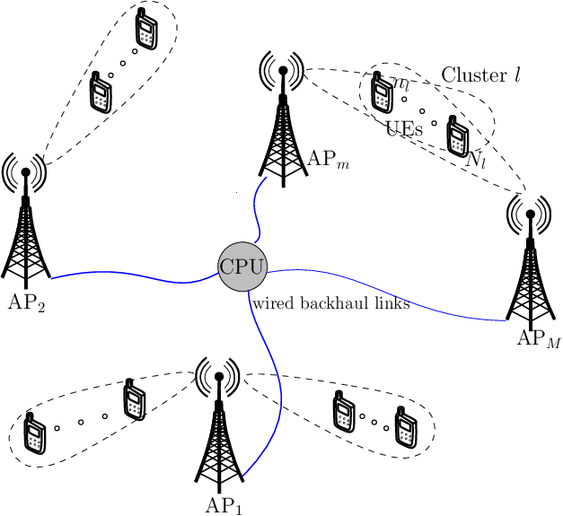
Fig. 1: An illustration of the CFmMIMO-NOMA system.

We consider an CFmMIMO-NOMA system, where the set ℳ≜{1,2,⋯,M}\mathcal{M}\triangleq\{1,2,\cdots,M\} of MM APs are connected to the CPU through perfect wired backhaul links to serve the set 𝒩≜{1,2,⋯,N}\mathcal{N}\triangleq\{1,2,\cdots,N\} of NN UEs via a shared wireless medium, as shown in Fig. 1. Each AP is equipped with KK antennas, while each UE has a single antenna. APs and UEs are assumed to be randomly distributed in a wide coverage area. The communication between APs and UEs follows the time division duplex (TDD) mode. Each coherence interval, denoted by τc\tau_{c}, includes two phases: uplink training τp\tau_{p} (τp<τc\tau_{p}<\tau_{c}) and downlink data transmission (τc−τp\tau_{c}-\tau_{p}). The total NN UEs are grouped into LL clusters and each UE belongs to one cluster only. We denote the set of LL clusters by ℒ≜{1,2,⋯L}\mathcal{L}\triangleq\{1,2,\cdots L\}. The set of UEs in the ll-th cluster is defined as 𝒩l≜{1l,⋯,nl,⋯,Nl}\mathcal{N}_{l}\triangleq\{1_{l},\cdots,n_{l},\cdots,N_{l}\} with |𝒩l|=Nl|\mathcal{N}_{l}|=N_{l}, where ⋃l∈ℒ|𝒩l|=N\bigcup_{l\in\mathcal{L}}|\mathcal{N}_{l}|=N and 𝒩l​⋂𝒩l′=∅\mathcal{N}_{l}\bigcap\mathcal{N}_{l^{\prime}}=\emptyset for l≠l′l\neq{l^{\prime}}.

II-B Signal Model

II-B1 Uplink Training

In the uplink training phase, all UEs send their training pilots to APs for channel estimation. Then, downlink channels are achieved by leveraging the channel reciprocity property of the TDD mode. With the aim of minimizing the channel estimation overhead in CFmMIMO-NOMA, UEs in the same cluster share the same pilot sequence, and the pilot sequences among different clusters are pairwisely orthogonal [12, 16] which requires τp≥L\tau_{p}\geq L. In this paper, we assume that τp=L\tau_{p}=L. Let us denote the pilot sequence sent from the UEs in the ll-th cluster by ϕl∈ℂτp×1\boldsymbol{\phi}_{l}\in\mathbb{C}^{\tau_{p}\times 1} with l∈{1,2,…,τp}l\in\{1,2,\ldots,\tau_{p}\}, satisfying the orthogonality, i.e., ‖ϕl‖22=τp\|\boldsymbol{\phi}_{l}\|^{2}_{2}=\tau_{p} and ϕlH​ϕl′=0\boldsymbol{\phi}^{H}_{l}\boldsymbol{\phi}_{l^{\prime}}=0 if l≠l′l\neq{l^{\prime}}. The channel vector from UE nln_{l} to APm is defined as hm,nl∈ℂK×1\textbf{h}_{m,n_{l}}\in\mathbb{C}^{K\times 1}. In this paper, we focus on slowly time-varying channels, and assume that the channel coefficients are static during the τc\tau_{c} interval. The channel hm,nl\textbf{h}_{m,n_{l}} is generally modeled as follows:

hm,nl=βm,nl​h¯m,nl,\displaystyle\textbf{h}_{m,n_{l}}=\sqrt{\beta_{m,n_{l}}}\bar{\textbf{h}}_{m,n_{l}}, (1)

where βm,nl\beta_{m,n_{l}} represents the large-scale fading coefficient accounting for path loss and shadowing, and h¯m,nl∈ℂK×1\bar{\textbf{h}}_{m,n_{l}}\in\mathbb{C}^{K\times 1} is small-scale fading vector in which the components are independent and identically distributed (i.i.d.) 𝒞​𝒩​(0,1)\mathcal{CN}(0,1) RVs. The training signals received at APm can be written as follows:

Ymp=∑l∈ℒ∑nl∈𝒩lρnl​hm,nl​ϕlH+Wmp,\displaystyle\textbf{Y}^{p}_{m}=\sum\limits_{l\in\mathcal{L}}\sum\limits_{n_{l}\in\mathcal{N}_{l}}\sqrt{\rho_{n_{l}}}\textbf{h}_{m,n_{l}}\boldsymbol{\phi}_{l}^{H}+\textbf{W}^{p}_{m}, (2)

where ρnl\rho_{n_{l}} and Wmp∈ℂK×τp\textbf{W}^{p}_{m}\in\mathbb{C}^{K\times\tau_{p}} are the normalized transmit power of UE nl{n_{l}} and the additive noise matrix at APm whose elements follow 𝒞​𝒩​(0,1)\mathcal{CN}(0,1), respectively.

Given Ymp\textbf{Y}^{p}_{m}, APm estimates hm,nl\textbf{h}_{m,n_{l}} using the minimum mean square error (MMSE) criterion. The projection y^mp∈ℂK×1\hat{\textbf{y}}^{p}_{m}\in\mathbb{C}^{K\times 1} of Ymp\textbf{Y}^{p}_{m} at APm onto ϕl\boldsymbol{\phi}_{l} can be derived as follows:

y^mp=Ymp​ϕl=τp​∑nl∈𝒩lρnl​hm,nl+Wmp​ϕl.\displaystyle\hat{\textbf{y}}^{p}_{m}=\textbf{Y}^{p}_{m}\boldsymbol{\phi}_{l}=\tau_{p}\sum\limits_{n_{l}\in\mathcal{N}_{l}}\sqrt{\rho_{n_{l}}}\textbf{h}_{m,n_{l}}+\textbf{W}^{p}_{m}\boldsymbol{\phi}_{l}. (3)

Hence, the MMSE estimate of hm,nl\textbf{h}_{m,n_{l}} is given as

h^m,nl=𝔼⁡{hm,nl​(y^mp)H}𝔼⁡{y^mp​(y^mp)H}​y^mp=υm,nl​y^mp,\displaystyle\hat{\textbf{h}}_{m,n_{l}}=\frac{\mathbb{E}\{\textbf{h}_{m,n_{l}}(\hat{\textbf{y}}^{p}_{m})^{H}\}}{\mathbb{E}\{\hat{\textbf{y}}^{p}_{m}(\hat{\textbf{y}}^{p}_{m})^{H}\}}\hat{\textbf{y}}^{p}_{m}=\upsilon_{m,n_{l}}\hat{\textbf{y}}^{p}_{m}, (4)

where υm,nl=ρnl​βm,nlτp​∑n′l∈𝒩lρn′l​βm,n′l+1\displaystyle\upsilon_{m,n_{l}}=\frac{\sqrt{\rho_{n_{l}}}\beta_{m,n_{l}}}{\tau_{p}\sum\limits_{{n^{\prime}}_{l}\in\mathcal{N}_{l}}\rho_{{n^{\prime}}_{l}}\beta_{m,{n^{\prime}}_{l}}+1}. The estimation error vector of hm,nl\textbf{h}_{m,n_{l}} is given as

em,nl=hm,nl−h^m,nl,\displaystyle\textbf{e}_{m,n_{l}}=\textbf{h}_{m,n_{l}}-\hat{\textbf{h}}_{m,n_{l}}, (5)

where em,nl\textbf{e}_{m,n_{l}} and h^m,nl\hat{\textbf{h}}_{m,n_{l}} are i.i.d. RVs distributed as 𝒞​𝒩\mathcal{CN} (0,(βm,nl−γm,nl)​IK)(\textbf{0},\left(\beta_{m,n_{l}}-\gamma_{m,n_{l}}\right)\textbf{I}_{K}) and 𝒞​𝒩\mathcal{CN} (0,γm,nl​IK)(\textbf{0},\gamma_{m,n_{l}}\textbf{I}_{K}), respectively, with γm,nl=τp​ρnl​βm,nl2τp​∑n′l∈𝒩lρn′l​βm,n′l+1\displaystyle\gamma_{m,n_{l}}=\frac{\tau_{p}\rho_{n_{l}}\beta^{2}_{m,n_{l}}}{\tau_{p}\sum\limits_{{n^{\prime}}_{l}\in\mathcal{N}_{l}}\rho_{{n^{\prime}}_{l}}\beta_{m,{n^{\prime}}_{l}}+1}. Note that there is no cooperation among APs to exchange the channel estimate information.

Remark 1.

The so-called pilot contamination exists when APs estimate the channels of UEs belonging to the same cluster. The relationship of channel estimates of UE nl{n_{l}} and UE n′l{{n^{\prime}}_{l}} in the ll-th cluster with nl≠n′ln_{l}\neq{n^{\prime}}_{l} and nl,n′l∈𝒩ln_{l},{n^{\prime}}_{l}\in\mathcal{N}_{l}, at APm is expressed as follows:

h^m,nl=ρnl​βm,nlρn′l​βm,n′l​h^m,n′l.\displaystyle\hat{\textbf{h}}_{m,n_{l}}=\frac{\sqrt{\rho_{n_{l}}}\beta_{m,n_{l}}}{\sqrt{\rho_{{n^{\prime}}_{l}}}\beta_{m,{n^{\prime}}_{l}}}\hat{\textbf{h}}_{m,{n^{\prime}}_{l}}. (6)

II-B2 Downlink Data Transmission

Under TDD operation, we consider the channel reciprocity to acquire CSI to precode the transmit signals in the downlink [9, 6]. In this paper, we adopt fpZF precoding [28] to cancel inter-cluster interference, but still take into account intra-cluster interference. Compared with the pure ZF [29], each AP computes fpZF precoding using its local CSI only, leading to an implementable algorithm. From (2), the full-rank matrix H~m∈ℂK×τp\tilde{\textbf{H}}_{m}\in\mathbb{C}^{K\times\tau_{p}} of fpZF precoder at APm is given by [28]

H~m=Ymp​ϕ,\displaystyle\tilde{\textbf{H}}_{m}=\textbf{Y}^{p}_{m}\boldsymbol{\phi}, (7)

where ϕ=[ϕ1,ϕ2,⋯,ϕτp]∈ℂτp×τp\boldsymbol{\phi}=[\boldsymbol{\phi}_{1},\boldsymbol{\phi}_{2},\cdots,\boldsymbol{\phi}_{\tau_{p}}]\in\mathbb{C}^{\tau_{p}\times\tau_{p}} denotes the collection of τp\tau_{p} orthogonal pilot sequences. Hence, from (4) and (7), the channel estimate h^m,nl\hat{\textbf{h}}_{m,n_{l}} is rewritten as

h^m,nl=υm,nl​H~m​𝝋l,\displaystyle\hat{\textbf{h}}_{m,n_{l}}=\upsilon_{m,n_{l}}\tilde{\textbf{H}}_{m}\boldsymbol{\varphi}_{l}, (8)

where 𝝋l\boldsymbol{\varphi}_{l} is the ll-th column of the identity matrix Iτp\textbf{I}_{\tau_{p}}. From (7) and (8), the beamforming vector 𝒘m,l∈ℂK×1\boldsymbol{w}_{m,l}\in\mathbb{C}^{K\times 1} oriented to the ll-th cluster at APm can be expressed as follows:

𝒘m,l=H~m​(H~mH​H~m)−1​𝝋l𝔼⁡{‖H~m​(H~mH​H~m)−1​𝝋l‖22}.\displaystyle\boldsymbol{w}_{m,l}=\frac{\tilde{\textbf{H}}_{m}\bigl(\tilde{\textbf{H}}_{m}^{H}\tilde{\textbf{H}}_{m}\bigr)^{-1}\boldsymbol{\varphi}_{l}}{\sqrt{\mathbb{E}\left\{\bigr\|\tilde{\textbf{H}}_{m}\bigl(\tilde{\textbf{H}}_{m}^{H}\tilde{\textbf{H}}_{m}\bigr)^{-1}\boldsymbol{\varphi}_{l}\bigl\|^{2}_{2}\right\}}}. (9)

The transmitted signal 𝒙m∈ℂK×1\boldsymbol{x}_{m}\in\mathbb{C}^{K\times 1} from APm is given by

𝒙m=∑l∈ℒ∑nl∈𝒩lρnlm​𝒘m,l​xnl,\displaystyle\boldsymbol{x}_{m}=\sum\limits_{l\in\mathcal{L}}\sum\limits_{n_{l}\in\mathcal{N}_{l}}\sqrt{\rho^{m}_{n_{l}}}\boldsymbol{w}_{m,l}x_{n_{l}}, (10)

where xnlx_{n_{l}} is the symbol intended for UE nln_{l}, and ρnlm\rho^{m}_{n_{l}} is the normalized transmit power (normalized by the noise power at APm) allocated to UE nln_{l} at APm. Besides, xnlx_{n_{l}} and xn′l′x_{{n^{\prime}}_{l^{\prime}}} for l,l′∈ℒl,{l^{\prime}}\in\mathcal{L} and nl,n′l′∈𝒩n_{l},{n^{\prime}}_{l^{\prime}}\in\mathcal{N} must satisfy the following condition

𝔼⁡{xnl​(xn′l′)∗}={1,ifl=l′andn=n′,0,otherwise.\displaystyle\mathbb{E}\bigl\{x_{n_{l}}(x_{{n^{\prime}}_{l^{\prime}}})^{*}\bigr\}=\begin{cases}1,&\text{if}\ \ l={l^{\prime}}\ \ \text{and}\ \ n={n^{\prime}},\\ 0,&\text{otherwise}.\end{cases} (11)

Then, the received signal at UE nl{n_{l}} in the ll-th cluster can be written as

ynl\displaystyle y_{n_{l}} =∑m∈ℳhm,nlH​𝒙m+znl\displaystyle=\sum\limits_{m\in\mathcal{M}}\textbf{h}_{m,n_{l}}^{H}\boldsymbol{x}_{m}+z_{n_{l}}
=∑m∈ℳρnlm​hm,nlH​𝒘m,l​xnl⏟Desired signal+∑m∈ℳ∑n′l∈𝒩l∖{nl}ρn′lm​hm,nlH​𝒘m,l​xn′l⏟Intra-cluster interference before SIC\displaystyle=\underbrace{\sum\limits_{m\in\mathcal{M}}\sqrt{\rho^{m}_{n_{l}}}\textbf{h}_{m,n_{l}}^{H}\boldsymbol{w}_{m,l}x_{n_{l}}}_{\text{Desired signal}}+\underbrace{\sum\limits_{m\in\mathcal{M}}\sum\limits_{{n^{\prime}}_{l}\in\mathcal{N}_{l}\setminus\{n_{l}\}}\sqrt{\rho^{m}_{{n^{\prime}}_{l}}}\textbf{h}_{m,n_{l}}^{H}\boldsymbol{w}_{m,l}x_{{n^{\prime}}_{l}}}_{\text{Intra-cluster interference before SIC}}
+∑m∈ℳ∑l′∈ℒ∖{l}∑nl′∈𝒩l′ρnl′m​hm,nlH​𝒘m,l′​xnl′⏟Inter-cluster interference+znl,\displaystyle\quad+\underbrace{\sum\limits_{m\in\mathcal{M}}\sum\limits_{{l^{\prime}}\in\mathcal{L}\setminus\{l\}}\sum\limits_{n_{l^{\prime}}\in\mathcal{N}_{l^{\prime}}}\sqrt{\rho^{m}_{{n}_{l^{\prime}}}}\textbf{h}_{m,n_{l}}^{H}\boldsymbol{w}_{m,{l^{\prime}}}x_{{n}_{l^{\prime}}}}_{\text{Inter-cluster interference}}+z_{n_{l}}, (12)

where znl∼𝒞​𝒩​(0,1)z_{n_{l}}\sim\mathcal{CN}(0,1) is the additive white Gaussian noise (AWGN) at UE nl{n_{l}}.

Without loss of generality, in the ll-th cluster we consider a descending order of channel gain, i.e., UEs 1l1_{l} and NlN_{l} are the users with strongest and weakest channel gains, respectively. By NOMA principle [4, 3], UE nln_{l} in the ll-th cluster first decodes the signals of UEs n′l>nl{n^{\prime}}_{l}>n_{l} with poorer channel conditions, and then its own signal is successively decoded after removing the interference from those UEs. Denote by SINRnln′l\text{SINR}^{{n^{\prime}}_{l}}_{n_{l}} and SINRn′ln′l\text{SINR}^{{n^{\prime}}_{l}}_{{n^{\prime}}_{l}} the signal-to-interference-plus-noise ratios (SINRs) in decoding the signal of UE n′l{n^{\prime}}_{l} by UE nln_{l} and itself, respectively. Towards an efficient and implementable SIC, the following necessary condition is considered [16]

𝔼{log2(1+SINRnln′l)}≥𝔼{log2(1+SINRn′ln′l)},∀nl<n′l,∀l∈ℒ.\displaystyle\mathbb{E}\left\{\text{log}_{2}\bigl(1+\text{SINR}^{{n^{\prime}}_{l}}_{n_{l}}\bigr)\right\}\geq\mathbb{E}\left\{\text{log}_{2}\bigr(1+\text{SINR}^{{n^{\prime}}_{l}}_{{n^{\prime}}_{l}}\bigl)\right\},\ \forall n_{l}<{n^{\prime}}_{l},\forall l\in\mathcal{L}. (13)
Remark 2.

We note that perfect SIC is practically unattainable owing to the effects of intra-cluster pilot contamination and channel estimation errors. Consequently, the received signal at UE nl{n_{l}} in the ll-th cluster after SIC processing can be written as follows:

y¯nl\displaystyle\bar{y}_{n_{l}} =∑m∈ℳρnlm​hm,nlH​𝒘m,l​xnl⏟Desired signal+∑m∈ℳ∑n′l=1nl−1ρn′lm​hm,nlH​𝒘m,l​xn′l⏟Intra-cluster interference after SIC\displaystyle=\underbrace{\sum\limits_{m\in\mathcal{M}}\sqrt{\rho^{m}_{n_{l}}}\textbf{h}_{m,n_{l}}^{H}\boldsymbol{w}_{m,l}x_{n_{l}}}_{\text{Desired signal}}+\underbrace{\sum\limits_{m\in\mathcal{M}}\sum\limits_{{n^{\prime}}_{l}=1}^{n_{l}-1}\sqrt{\rho^{m}_{{n^{\prime}}_{l}}}\textbf{h}_{m,n_{l}}^{H}\boldsymbol{w}_{m,l}x_{{n^{\prime}}_{l}}}_{\text{Intra-cluster interference after SIC}}
+ζnl​∑m∈ℳ∑n′′l=nl+1Nlρn′′lm​hm,nlH​𝒘m,l​xn′′l⏟Intra-cluster interference due to imperfect SIC+∑m∈ℳ∑l′∈ℒ∖{l}∑nl′∈𝒩l′ρnl′m​hm,nlH​𝒘m,l′​xnl′⏟Inter-cluster interference+znl,\displaystyle+\underbrace{\sqrt{\zeta_{{n}_{l}}}\sum\limits_{m\in\mathcal{M}}\sum\limits_{{n^{\prime\prime}}_{l}=n_{l}+1}^{N_{l}}\sqrt{\rho^{m}_{{n^{\prime\prime}}_{l}}}\textbf{h}_{m,n_{l}}^{H}\boldsymbol{w}_{m,l}x_{{n^{\prime\prime}}_{l}}}_{\text{Intra-cluster interference due to imperfect SIC}}+\underbrace{\sum\limits_{m\in\mathcal{M}}\sum\limits_{{l^{\prime}}\in\mathcal{L}\setminus\{l\}}\sum\limits_{n_{l^{\prime}}\in\mathcal{N}_{l^{\prime}}}\sqrt{\rho^{m}_{{n}_{l^{\prime}}}}\textbf{h}_{m,n_{l}}^{H}\boldsymbol{w}_{m,{l^{\prime}}}x_{{n}_{l^{\prime}}}}_{\text{Inter-cluster interference}}+z_{n_{l}}, (14)

where ζnl\zeta_{{n}_{l}} is a general SIC performance coefficient at UE nl{n_{l}} in the ll-th cluster. In particular, ζnl=1\zeta_{{n}_{l}}=1 (ζnl=0\zeta_{{n}_{l}}=0) indicates no SIC (perfect SIC), while 0<ζnl<10<\zeta_{{n}_{l}}<1 means imperfect SIC.

III Clustering Cell-Free Massive MIMO-NOMA System

In this section, we propose two unsupervised ML-based UC algorithms to effectively divide all UEs into separate clusters, which are done at the CPU by exploiting the large-scale fading coefficients. Similarly to [16] and [25], large-scale fading coefficients of UEs are assumed to be collected and shared with the CPU before performing UC algorithms. We note that it is only necessary to estimate the large-scale fading coefficients once every 40 τc\tau_{c} intervals [12], and thus conveying these coefficients via the backhaul links occurs much less frequently than data transmission. Denote by 𝜷n≜[β1,n,β2,n,…,βM,n]T∈ℝM×1\boldsymbol{\beta}_{n}\triangleq[\beta_{1,n},\beta_{2,n},\ldots,\beta_{M,n}]^{T}\in\mathbb{R}^{M\times 1} the set of large-scale fading coefficients from all APs associated to UE n,∀n∈𝒩n,\forall n\in\mathcal{N}. The vector 𝜷n\boldsymbol{\beta}_{n} can be considered as an effective feature-vector denoting the location of UE nn.

III-A The k-means Algorithm

The k-means algorithm for UC studied in[24] and [25] is one of the simplest unsupervised ML algorithms to partition UEs in the coverage area into separate groups. The key idea is to find a user-specified number of clusters LL, which are represented by LL centroids, one for each cluster. The number of clusters LL in the k-means algorithm can be predetermined. The principle of k-means algorithm is given as follows. Firstly, LL initial centroids are randomly selected. Secondly, each point is assigned to the nearest centroid, and each mass of points assigned to the same centroid creates a cluster. Then, the centroid of each cluster is updated according to the points associated to the cluster. The assignment and update processes of centroids are repeated until either there is no change in the clusters or centroids remain similarly.

In the context of CFmMIMO-NOMA, the procedure of k-means can be summarized as follows:

  • •

    Step 1: LL initial centroids are randomly selected from NN UEs, where LL is a predefined number. Let us define the set of LL cluster centroids as follows:

    𝒞={cl,l∈ℒ},\displaystyle\mathcal{C}=\left\{c_{l},l\in\mathcal{L}\right\}, (15)

    where clc_{l} represents the centroid of the ll-th cluster.

  • •

    Step 2: Each UE n∈𝒩n\in\mathcal{N} is grouped to the nearest centroid, and hence, UEs assigned to the same centroid creates a cluster:

    l′=arg⁡min∀l∈ℒ⁡fd​(𝜷n,𝜷cl),\displaystyle{l^{\prime}}=\mathop{\arg\min}\limits_{\forall l\in\mathcal{L}}f_{d}\left(\boldsymbol{\beta}_{n},\boldsymbol{\beta}_{c_{l}}\right), (16)

    where fd​(𝜷n,𝜷cl)=‖𝜷n−𝜷cl‖2f_{d}\left(\boldsymbol{\beta}_{n},\boldsymbol{\beta}_{c_{l}}\right)={\|\boldsymbol{\beta}_{n}-\boldsymbol{\beta}_{c_{l}}\|}_{2} represents the Euclidean distance from UE nn to centroid clc_{l}. As shown in (16), UE nn is grouped to l′l^{\prime}-th cluster (denoted by centroid cl′c_{l^{\prime}}) since the distance from UE nn to centroid cl′c_{l^{\prime}} is nearest.

  • •

    Step 3: The centroid of each cluster is recalculated under given UEs assigned to this cluster:

    𝜷cl=1|𝒩l|​∑n∈𝒩l𝜷n,∀l∈ℒ,\displaystyle\boldsymbol{\beta}_{c_{l}}=\frac{1}{|\mathcal{N}_{l}|}\sum\limits_{n\in\mathcal{N}_{l}}\boldsymbol{\beta}_{n},\forall l\in\mathcal{L}, (17)

    where 𝜷cl\boldsymbol{\beta}_{c_{l}} represents the updated centroid for the ll-th cluster, which can be calculated by the mean of all UEs belonging to the ll-th cluster.

  • •

    Step 4: Steps 2-3 are repeated until convergence, i.e., there is no change in the clusters or the centroids remain the same.

The k-means algorithm for UC in CFmMIMO-NOMA is given in Algorithm 1. Note that k-means is a greedy algorithm, which can converge to a local minimum since its performance highly depends on the predefined number of clusters LL and the centroid initialization process, i.e., how to select LL initial centroids.

1:  Input: LL and 𝜷n,∀n∈𝒩\boldsymbol{\beta}_{n},\forall n\in\mathcal{N}.
2:  //**Identify LL cluster centroids at random clc_{l}, ∀l∈ℒ\forall l\in\mathcal{L} (Step 1)**//
3:  Set 𝒞=∅\mathcal{C}=\emptyset and l=1l=1, where 𝒞\mathcal{C} denotes the set of cluster centroids.
4:  while l≤Ll\leq L do
5:   cl=𝗀𝖾𝗇𝖾𝗋𝖺𝗍𝖾𝖱𝖺𝗇𝖽𝗈𝗆⁡[𝟣,N]c_{l}=\sf{generateRandom}[1,\textit{N}];
6:   if cl∉𝒞c_{l}\not\in\mathcal{C} then
7:    𝒞←cl\mathcal{C}\leftarrow c_{l};
8:    l=l+1l=l+1;
9:   end if
10:  end while
11:  //**Main process**//
12:  while 𝒞\mathcal{C} changes do
13:   //**Identify 𝒩l′\mathcal{N}_{l^{\prime}}, ∀l′∈ℒ\forall{l^{\prime}}\in\mathcal{L}, containing the subset of UEs that are closer to cl′c_{l^{\prime}} than clc_{l}, with l′≠l{l^{\prime}}\neq l (Step 2)**//
14:   for n∈𝒩\𝒞n\in\mathcal{N}\backslash\mathcal{C} do
15:    l′=arg⁡min∀l∈ℒ⁡fd​(𝜷n,𝜷cl){l^{\prime}}=\mathop{\arg\min}\limits_{\forall l\in\mathcal{L}}f_{d}\left(\boldsymbol{\beta}_{n},\boldsymbol{\beta}_{c_{l}}\right), where fd​(𝜷n,𝜷cl)=‖𝜷n−𝜷cl‖2f_{d}\left(\boldsymbol{\beta}_{n},\boldsymbol{\beta}_{c_{l}}\right)={||\boldsymbol{\beta}_{n}-\boldsymbol{\beta}_{c_{l}}||}_{2};
16:    𝒩l′←n\mathcal{N}_{l^{\prime}}\leftarrow n;
17:   end for
18:   //**Recalculate clc_{l} of cluster 𝒩l\mathcal{N}_{l}, ∀l∈ℒ\forall l\in\mathcal{L} (Step 3)**//
19:   for l=1:Ll=1:L do
20:    𝜷cl=1|𝒩l|​∑n∈𝒩l𝜷n\boldsymbol{\beta}_{c_{l}}=\frac{1}{|\mathcal{N}_{l}|}\sum\limits_{n\in\mathcal{N}_{l}}\boldsymbol{\beta}_{n};
21:   end for
22:  end while
23:  Output: 𝒩l\mathcal{N}_{l} and clc_{l}, ∀l∈ℒ\forall l\in\mathcal{L}.
Algorithm 1 The k-means Algorithm for UC in CFmMIMO-NOMA.

III-B Proposed k-means++ Algorithm

One drawback of the k-means algorithm is that it is sensitive to the initialization of the centroids [30, 31]. If an initial centroid is a far point, it might not associate with any other points. Equivalently, more than one initial centroids might be created into the same cluster which leads to poor grouping. In this section, the k-means++ algorithm is developed to resolve this issue. It aims at providing a clever initialization of the centroids that improves the quality of the grouping process. Except for the improvement in the centroid initialization process, the remainder of k-means++ algorithm is the same as in the k-means. In the context of CFmMIMO-NOMA, the procedure of proposed k-means++ can be summarized as follows:

  • •

    Step 1: The first initial centroid c1c_{1} is randomly selected from NN UEs.

  • •

    Step 2: For each UE nn (with n∈𝒩​and​n∉𝒞n\in\mathcal{N}\ \text{and}\ n\not\in\mathcal{C}), its distance from the nearest centroid is calculated as follows:

    fd​(𝜷n,𝜷ct)=‖𝜷n−𝜷ct‖2,\displaystyle f_{d}\left(\boldsymbol{\beta}_{n},\boldsymbol{\beta}_{c_{t}}\right)={\|\boldsymbol{\beta}_{n}-\boldsymbol{\beta}_{c_{t}}\|}_{2}, (18)

    where ct=arg⁡min∀cl∈𝒞⁡fd​(𝜷n,𝜷cl){c_{t}}=\mathop{\arg\min}\limits_{\forall c_{l}\in\mathcal{C}}f_{d}\left(\boldsymbol{\beta}_{n},\boldsymbol{\beta}_{c_{l}}\right).

  • •

    Step 3: The next centroid is selected from UEs (∀n∈𝒩\𝒞)(\forall n\in\mathcal{N}\backslash\mathcal{C}) such that the probability of selecting a UE as a centroid is in direct proportion to its distance from the nearest and previously selected centroid, i.e., the UE having the maximum distance from the nearest centroid is virtually to be chosen next as a centroid:

    cl=arg⁡max∀n∈𝒩\𝒞⁡fd​(𝜷n,𝜷ct).\displaystyle c_{l}=\mathop{\arg\max}\limits_{\forall n\in\mathcal{N}\backslash\mathcal{C}}f_{d}\left(\boldsymbol{\beta}_{n},\boldsymbol{\beta}_{c_{t}}\right). (19)
  • •

    Step 4: Steps 2-3 are repeated until L−1L-1 centroids are selected.

  • •

    The remaining process follows Steps 2-4 in the k-means algorithm.

The centroid initialization process of the proposed k-means++ ensures that chosen centroids are far away from each other. This increases the opportunity of initially selecting centroids that are located in different clusters. The proposed k-means++ algorithm for UC in CFmMIMO-NOMA is described in Algorithm 2.

1:  Input: LL and 𝜷n\boldsymbol{\beta}_{n}, ∀n∈𝒩\forall n\in\mathcal{N}.
2:  Set 𝒞=∅\mathcal{C}=\emptyset and c1=𝗀𝖾𝗇𝖾𝗋𝖺𝗍𝖾𝖱𝖺𝗇𝖽𝗈𝗆⁡[𝟣,N]c_{1}=\sf{generateRandom}[1,\textit{N}];
3:  𝒞←c1\mathcal{C}\leftarrow c_{1} and set f=0f=0;
4:  for l=2:Ll=2:L do
5:   for n=1:Nn=1:N do
6:    for t=1:l−1t=1:l-1 do
7:     if nn ≠\neq ctc_{t} then
8:      d​i​s​(1,t)=fd​(𝜷n,𝜷ct)dis\left(1,t\right)=f_{d}\left(\boldsymbol{\beta}_{n},\boldsymbol{\beta}_{c_{t}}\right), where fd​(𝜷n,𝜷ct)=‖𝜷n−𝜷ct‖2f_{d}\left(\boldsymbol{\beta}_{n},\boldsymbol{\beta}_{c_{t}}\right)={\|\boldsymbol{\beta}_{n}-\boldsymbol{\beta}_{c_{t}}\|}_{2};
9:     else
10:      d​i​s​(1,t)=NaNdis\left(1,t\right)=\rm{NaN};
11:      f=f+1f=f+1;
12:     end if
13:    end for
14:    if f==0f==0 then
15:     d​i​s​t​(1,n)=max​disdist\left(1,n\right)=\rm{max}\ \textit{dis};
16:    else
17:     d​i​s​t​(1,n)=NaNdist\left(1,n\right)=\rm{NaN};
18:     f=0f=0;
19:    end if
20:   end for
21:   cl=arg⁡max∀n∈𝒩\𝒞⁡distc_{l}=\mathop{\arg\max}\limits_{\forall n\in\mathcal{N}\backslash\mathcal{C}}\textit{dist};
22:   𝒞←cl\mathcal{C}\leftarrow c_{l};
23:  end for
24:  while 𝒞\mathcal{C} changes do
25:   for n∈𝒩\𝒞n\in\mathcal{N}\backslash\mathcal{C} do
26:    l′=arg⁡min∀l∈ℒ⁡fd​(𝜷n,𝜷cl){l^{\prime}}=\mathop{\arg\min}\limits_{\forall l\in\mathcal{L}}f_{d}\left(\boldsymbol{\beta}_{n},\boldsymbol{\beta}_{c_{l}}\right), where fd​(𝜷n,𝜷cl)=‖𝜷n−𝜷cl‖2f_{d}\left(\boldsymbol{\beta}_{n},\boldsymbol{\beta}_{c_{l}}\right)={\|\boldsymbol{\beta}_{n}-\boldsymbol{\beta}_{c_{l}}\|}_{2};
27:    𝒩l′←n\mathcal{N}_{l^{\prime}}\leftarrow n;
28:   end for
29:   for l=1:Ll=1:L do
30:    𝜷cl=1|𝒩l|​∑n∈𝒩l𝜷n\boldsymbol{\beta}_{c_{l}}=\frac{1}{|\mathcal{N}_{l}|}\sum\limits_{n\in\mathcal{N}_{l}}\boldsymbol{\beta}_{n};
31:   end for
32:  end while
33:  Output: 𝒩l\mathcal{N}_{l} and clc_{l}, ∀l∈ℒ\forall l\in\mathcal{L}.
Algorithm 2 The k-means++ Algorithm for UC in CFmMIMO-NOMA.

III-C The Improved k-means++ Algorithm

As shown in Sections III-A and III-B, the performance of the k-means algorithm can be enhanced by selecting LL initial centroids more effectively. Based on the characteristics of CFmMIMO-NOMA, we propose the improved k-means++ algorithm which includes a new approach to cleverly select LL initial centroids. The procedure of improved k-means++ is summarized as follows:

  • •

    Step 1: Each AP identifies an associated UE, denoted by Λm\Lambda_{m}, which has the best connection, i.e., highest large-scale fading coefficient βm,n\beta_{m,n}:

    Λm=arg⁡max∀n∈𝒩⁡βm,n,∀m∈ℳ.\displaystyle\Lambda_{m}=\mathop{\arg\max}\limits_{\forall n\in\mathcal{N}}\beta_{m,n},\forall m\in\mathcal{M}. (20)
  • •

    Step 2: The CPU then selects a subset of APs, denoted by Υn\Upsilon_{n}, which have best connections to UE nn:

    Υn={APm:UE​n==Λm},∀n∈𝒩.\displaystyle\Upsilon_{n}=\left\{\text{AP}_{m}:\text{UE}\ {n}==\Lambda_{m}\right\},\forall n\in\mathcal{N}. (21)
  • •

    Step 3: The CPU selects a UE having the highest number of serving APs as a centroid:

    cl=arg⁡max∀n∈𝒩\𝒞⁡|Υn|,\displaystyle c_{l}=\mathop{\arg\max}\limits_{\forall n\in\mathcal{N}\backslash\mathcal{C}}|\Upsilon_{n}|, (22)

    where |Υn||\Upsilon_{n}| denotes the cardinality of Υn\Upsilon_{n}.

  • •

    Step 4: Step 3 is repeated until LL centroids are chosen.

  • •

    The remaining process follows Steps 2-4 in the k-means algorithm.

The centroid initialization process of the improved k-means++ for UC in CFmMIMO-NOMA is described in Algorithm 3.

1:  Input: LL and 𝜷n,∀n∈𝒩\boldsymbol{\beta}_{n},\forall n\in\mathcal{N}.
2:  for m=1:Mm=1:M do
3:   Λm=arg⁡max∀n∈𝒩⁡βm,n\Lambda_{m}=\mathop{\arg\max}\limits_{\forall n\in\mathcal{N}}\beta_{m,n};
4:  end for
5:  for n=1:Nn=1:N do
6:   for m=1:Mm=1:M do
7:    if n==Λmn==\Lambda_{m} then
8:     Υn←m\Upsilon_{n}\leftarrow m;
9:    end if
10:   end for
11:  end for
12:  𝒞=∅\mathcal{C}=\emptyset, where 𝒞\mathcal{C} denotes the set of cluster centroids.
13:  for l=1:Ll=1:L do
14:   cl=arg⁡max∀n∈𝒩\𝒞⁡|Υn|c_{l}=\mathop{\arg\max}\limits_{\forall n\in\mathcal{N}\backslash\mathcal{C}}|\Upsilon_{n}|;
15:   𝒞←cl\mathcal{C}\leftarrow c_{l};
16:  end for
17:  Output: 𝒞\mathcal{C}.
Algorithm 3 Centroid Initialization Process of the Improved k-means++ Algorithm for UC in CFmMIMO-NOMA.

III-D Complexity Analysis

As shown in [24], the complexity of the k-means algorithm is 𝒪⁡(N​L​I​M)\mathcal{O}\left(NLIM\right), where II denotes the total number of iterations until convergence. We recall that compared to the k-means, the k-means++ and improved k-means++ algorithms require the modification of centroid initialization process. All centroids in the k-means algorithm are randomly chosen, which leads to the computational complexity of 𝒪⁡(N)\mathcal{O}\left(N\right). The proposed k-means++ algorithm has to make a full search through all UEs for every centroid sampled, resulting to the complexity of 𝒪⁡(N​L​M)\mathcal{O}\left(NLM\right) [32]. Similarly, the complexity of the improved k-means++ algorithm is 𝒪⁡(M​N+N​M+L​N)\mathcal{O}\left(MN+NM+LN\right), which is lower than that of the k-means++. In addition, although the centroid initialization process in the proposed k-means++ algorithms is computationally more expensive than the original k-means, the performance of the former is much better than the latter. This will be elaborated in Section VII.

IV Performance Analysis

Given the UC algorithms in Section III, we now derive the SSE of CFmMIMO-NOMA. From (2), the SINR of UE nln_{l} in the ll-th cluster is given as

SINRnl=|DSnl|2𝔼⁡{|BUnl|2}+∑n′l=1nl−1𝔼⁡{|ICInl|2}+∑n′′l=nl+1Nl𝔼⁡{|RICInl|2}+∑l′∈ℒ∖{l}∑nl′∈𝒩l′𝔼⁡{|UInl|2}+1,\text{SINR}_{n_{l}}=\frac{|\text{DS}_{n_{l}}|^{2}}{\mathbb{E}\left\{|\text{BU}_{n_{l}}|^{2}\right\}+\sum\limits_{{n^{\prime}}_{l}=1}^{n_{l}-1}\mathbb{E}\left\{|\text{ICI}_{n_{l}}|^{2}\right\}+\sum\limits_{{n^{\prime\prime}}_{l}=n_{l}+1}^{N_{l}}\mathbb{E}\left\{|\text{RICI}_{n_{l}}|^{2}\right\}+\sum\limits_{{l^{\prime}}\in\mathcal{L}\setminus\{l\}}\sum\limits_{n_{l^{\prime}}\in\mathcal{N}_{l^{\prime}}}\mathbb{E}\left\{|\text{UI}_{n_{l}}|^{2}\right\}+1}, (23)

where DSnl=𝔼⁡{∑m∈ℳρnlm​hm,nlH​𝒘m,l}\text{DS}_{n_{l}}=\mathbb{E}\Bigl\{\sum\limits_{m\in\mathcal{M}}\sqrt{\rho^{m}_{n_{l}}}\textbf{h}_{m,n_{l}}^{H}\boldsymbol{w}_{m,l}\Bigr\}, BUnl=(∑m∈ℳρnlmhm,nlH𝒘m,l−𝔼{∑m∈ℳρnlmhm,nlH𝒘m,l})\text{BU}_{n_{l}}=\Bigl(\sum\limits_{m\in\mathcal{M}}\sqrt{\rho^{m}_{n_{l}}}\textbf{h}_{m,n_{l}}^{H}\boldsymbol{w}_{m,l}-\mathbb{E}\Bigl\{\sum\limits_{m\in\mathcal{M}}\sqrt{\rho^{m}_{n_{l}}}\textbf{h}_{m,n_{l}}^{H}\boldsymbol{w}_{m,l}\Bigl\}\Bigl), ICInl=∑m∈ℳρn′lm​hm,nlH​𝒘m,l\text{ICI}_{n_{l}}=\sum\limits_{m\in\mathcal{M}}\sqrt{\rho^{m}_{{n^{\prime}}_{l}}}\textbf{h}_{m,n_{l}}^{H}\boldsymbol{w}_{m,l}, RICInl=ζnl​∑m∈ℳρn′′lm​hm,nlH​𝒘m,l\text{RICI}_{n_{l}}=\sqrt{\zeta_{{n}_{l}}}\sum\limits_{m\in\mathcal{M}}\sqrt{\rho^{m}_{{n^{\prime\prime}}_{l}}}\textbf{h}_{m,n_{l}}^{H}\boldsymbol{w}_{m,l}, and UInl=∑m∈ℳρnl′m​hm,nlH​𝒘m,l′\text{UI}_{n_{l}}=\sum\limits_{m\in\mathcal{M}}\sqrt{\rho^{m}_{{n}_{l^{\prime}}}}\textbf{h}_{m,n_{l}}^{H}\boldsymbol{w}_{m,{l^{\prime}}} are coherent beamforming gain (desired signal), beamforming gain uncertainty, intra-cluster interference after SIC, residual interference due to imperfect SIC, and inter-cluster interference, respectively.

To simplify (23), we first compute the expectation term in the denominator of (9) [33]:

𝔼⁡{‖H~m​(H~mH​H~m)−1​𝝋l‖22}=υm,nl2γm,nl​(K−τp),∀nl∈𝒩l.\displaystyle\mathbb{E}\left\{\bigr\|\tilde{\textbf{H}}_{m}\bigl(\tilde{\textbf{H}}_{m}^{H}\tilde{\textbf{H}}_{m}\bigr)^{-1}\boldsymbol{\varphi}_{l}\bigl\|^{2}_{2}\right\}=\frac{\upsilon^{2}_{m,n_{l}}}{\gamma_{m,n_{l}}(K-\tau_{p})},\ \forall n_{l}\in\mathcal{N}_{l}. (24)

From (8), (9), and (24), we have

h^m,niH​𝒘m,l\displaystyle{\hat{\textbf{h}}}^{H}_{m,n_{i}}\boldsymbol{w}_{m,l} =υm,niυm,nl​𝝋iH​𝝋l​γm,nl​(K−τp)\displaystyle=\frac{\upsilon_{m,n_{i}}}{\upsilon_{m,n_{l}}}\boldsymbol{\varphi}^{H}_{i}\boldsymbol{\varphi}_{l}\sqrt{\gamma_{m,n_{l}}(K-\tau_{p})}
={γm,nl​(K−τp),ifi=l,0,ifi≠l.\displaystyle=\begin{cases}\sqrt{\gamma_{m,n_{l}}(K-\tau_{p})},&\text{if}\ \ {i=l},\\ 0,&\text{if}\ \ i\neq l.\end{cases} (25)
Lemma 1.

The closed-form expression for the SE of UE nl{n_{l}} in the ll-th cluster is given by

Rnl\displaystyle R_{n_{l}} =(1−τpτc)log2(1+SINRnl)\displaystyle=\Bigl(1-\frac{\tau_{p}}{\tau_{c}}\Bigr)\log_{2}\Bigl(1+\mathrm{SINR}_{n_{l}}\Bigl)
=(1−τpτc)log2(1+minn′l=1,…,nlSINRn′lnl),∀nl.\displaystyle=\Bigl(1-\frac{\tau_{p}}{\tau_{c}}\Bigl)\log_{2}\Bigl(1+\min_{{n^{\prime}}_{l}=1,\ldots,n_{l}}\mathrm{SINR}^{n_{l}}_{{n^{\prime}}_{l}}\Bigl),\ \forall n_{l}. (26)

By 𝛒≜{ρnlm}m∈ℳ,nl∈𝒩l,l∈ℒ\boldsymbol{\rho}\triangleq\{\rho^{m}_{n_{l}}\}_{m\in\mathcal{M},n_{l}\in\mathcal{N}_{l},l\in\mathcal{L}}, SINRnlnl\mathrm{SINR}^{n_{l}}_{n_{l}} and SINRn′lnl\mathrm{SINR}^{n_{l}}_{{n^{\prime}}_{l}}, ∀n′l<nl\forall{n^{\prime}}_{l}<n_{l}, are derived as follows:

SINRnlnl=(K−τp)(∑m∈ℳρnlm​γm,nl)2ℐnlnl​(𝝆)+1,\displaystyle\mathrm{SINR}^{n_{l}}_{n_{l}}=\frac{(K-\tau_{p})\Bigl(\sum\limits_{m\in\mathcal{M}}\sqrt{\rho^{m}_{n_{l}}\gamma_{m,n_{l}}}\Bigl)^{2}}{\mathcal{I}^{n_{l}}_{n_{l}}(\boldsymbol{\rho})+1}, (27)
SINRn′lnl=(K−τp)​(∑m∈ℳρnlm​γm,n′l)2ℐn′lnl​(𝝆)+1,\displaystyle\mathrm{SINR}^{n_{l}}_{{n^{\prime}}_{l}}=\frac{(K-\tau_{p})\Bigl(\sum\limits_{m\in\mathcal{M}}\sqrt{\rho^{m}_{n_{l}}\gamma_{m,{n^{\prime}}_{l}}}\Bigr)^{2}}{\mathcal{I}^{n_{l}}_{{n^{\prime}}_{l}}(\boldsymbol{\rho})+1}, (28)

where ℐnlnl​(𝛒)\mathcal{I}^{n_{l}}_{n_{l}}(\boldsymbol{\rho}) and ℐn′lnl​(𝛒)\mathcal{I}^{n_{l}}_{{n^{\prime}}_{l}}(\boldsymbol{\rho}) are defined as

ℐnlnl​(𝝆)\displaystyle\mathcal{I}^{n_{l}}_{n_{l}}(\boldsymbol{\rho}) ≜∑n′′l∈𝒩l∖{nl}ηn′′l′​(K−τp)​(∑m∈ℳρn′′lm​γm,nl)2\displaystyle\triangleq\sum\limits_{{n^{\prime\prime}}_{l}\in\mathcal{N}_{l}\setminus\{n_{l}\}}\eta_{{n^{\prime\prime}}_{l^{\prime}}}(K-\tau_{p})\Bigl(\sum\limits_{m\in\mathcal{M}}\sqrt{\rho^{m}_{{n^{\prime\prime}}_{l}}\gamma_{m,n_{l}}}\Bigr)^{2}
+∑l′∈ℒ∑n′′l′∈𝒩l′∑m∈ℳηn′′l′ρn′′l′m(βm,nl−γm,nl),\displaystyle+\sum\limits_{{l^{\prime}}\in\mathcal{L}}\sum\limits_{{n^{\prime\prime}}_{l^{\prime}}\in\mathcal{N}_{l^{\prime}}}\sum\limits_{m\in\mathcal{M}}\eta_{{n^{\prime\prime}}_{l^{\prime}}}\rho^{m}_{{n^{\prime\prime}}_{l^{\prime}}}\left(\beta_{m,n_{l}}-\gamma_{m,n_{l}}\right),
ℐn′lnl​(𝝆)\displaystyle\mathcal{I}^{n_{l}}_{{n^{\prime}}_{l}}(\boldsymbol{\rho}) ≜∑n′′l∈𝒩l∖{nl}ηn′′l′(K−τp)(∑m∈ℳρn′′lm​γm,n′l)2\displaystyle\triangleq\sum\limits_{{n^{\prime\prime}}_{l}\in\mathcal{N}_{l}\setminus\{n_{l}\}}\eta_{{n^{\prime\prime}}_{l^{\prime}}}(K-\tau_{p})\Bigr(\sum\limits_{m\in\mathcal{M}}\sqrt{\rho^{m}_{{n^{\prime\prime}}_{l}}\gamma_{m,{n^{\prime}}_{l}}}\Bigl)^{2}
+∑l′∈ℒ∑n′′l′∈𝒩l′∑m∈ℳηn′′l′ρn′′l′m(βm,n′l−γm,n′l),\displaystyle+\sum\limits_{{l^{\prime}}\in\mathcal{L}}\sum\limits_{{n^{\prime\prime}}_{l^{\prime}}\in\mathcal{N}_{l^{\prime}}}\sum\limits_{m\in\mathcal{M}}\eta_{{n^{\prime\prime}}_{l^{\prime}}}\rho^{m}_{{n^{\prime\prime}}_{l^{\prime}}}\left(\beta_{m,{n^{\prime}}_{l}}-\gamma_{m,{n^{\prime}}_{l}}\right),

with

ηn′′l′={1,if​l′≠l​or​l′=l​and​n′′l≤nl,ζnl,otherwise.\eta_{{n^{\prime\prime}}_{l^{\prime}}}=\begin{cases}1,&\text{if}\ {l^{\prime}}\ \neq\ l\ \text{or}\ {l^{\prime}}\ =\ l\ \text{and}\ {n^{\prime\prime}}_{l}\ \leq\ {n}_{l},\\ \zeta_{{n}_{l}},&\text{otherwise}.\\ \end{cases}
Proof.

The proof is given in Appendix A. ∎

We define the virtual channel of UE nl{n_{l}} in the ll-th cluster as hnl=[γ1,nl,…,γM,nl]T\textbf{h}_{n_{l}}=\left[\gamma_{1,n_{l}},\ldots,\gamma_{M,n_{l}}\right]^{T}, ∀nl∈𝒩l\forall n_{l}\in\mathcal{N}_{l}. We assume that UEs in the ll-th cluster are sorted based on their virtual channels, such as ‖h1l‖2≥‖h2l‖2≥…≥‖hNl‖2\|\textbf{h}_{1_{l}}\|_{2}\geq\|\textbf{h}_{2_{l}}\|_{2}\geq\ldots\geq\|\textbf{h}_{N_{l}}\|_{2}, ∀l∈ℒ\forall l\in\mathcal{L}. From (1), the SSE of CFmMIMO-NOMA is expressed as

RΣ=∑l∈ℒ∑nl∈𝒩lRnl=(1−τpτc)∑l∈ℒ∑nl∈𝒩llog2(1+SINRnl).\displaystyle R_{\Sigma}=\sum\limits_{l\in\mathcal{L}}\sum\limits_{n_{l}\in\mathcal{N}_{l}}R_{n_{l}}=\Bigl(1-\frac{\tau_{p}}{\tau_{c}}\Bigr)\sum\limits_{l\in\mathcal{L}}\sum\limits_{n_{l}\in\mathcal{N}_{l}}\log_{2}\Bigl(1+\mathrm{SINR}_{n_{l}}\Bigl). (29)

From (27) and (28), it is clear that the SSE of CFmMIMO-NOMA highly depends on the power allocation (PA) at all APs. Thus, it is necessary to optimize the transmit power at APs so that the SSE of CFmMIMO-NOMA can be enhanced, which will be detailed next.

V The Sum Spectral Efficiency Maximization

We aim at optimizing the normalized transmit power 𝝆≜{ρnlm}m,nl,l\boldsymbol{\rho}\triangleq\{\rho^{m}_{n_{l}}\}_{m,n_{l},l} to maximize the SSE under the constraints of the transmit power budget at the APs and SIC conditions. The optimization problem can be mathematically expressed as

max𝝆\displaystyle\underset{\boldsymbol{\rho}}{\max} (1−τpτc)∑l∈ℒ∑nl∈𝒩llog2(1+SINRnl)\displaystyle\quad\Bigl(1-\frac{\tau_{p}}{\tau_{c}}\Bigr)\sum\limits_{l\in\mathcal{L}}\sum\limits_{n_{l}\in\mathcal{N}_{l}}\log_{2}\bigl(1+\mathrm{SINR}_{n_{l}}\bigl) (30a)
𝗌.𝗍.\displaystyle\mathsf{s.t.} ∑l∈ℒ∑nl∈𝒩lρnlm≤Pmaxm,∀m∈ℳ,\displaystyle\quad\sum\limits_{l\in\mathcal{L}}\sum\limits_{n_{l}\in\mathcal{N}_{l}}\rho^{m}_{n_{l}}\leq P^{m}_{\text{max}},\forall m\in\mathcal{M}, (30b)
ρnlm≤ρnl+1m,nl∈[1,Nl−1],∀m∈ℳ,l∈ℒ.\displaystyle\quad\rho^{m}_{n_{l}}\leq\rho^{m}_{n_{l}+1},n_{l}\in\left[1,N_{l}-1\right],\forall m\in\mathcal{M},l\in\mathcal{L}. (30c)

Herein, constraint (30b) indicates that the total transmit power at APm is limited by the normalized maximum power PmaxmP^{m}_{\text{max}}, while constraint (30c) is the necessary condition to implement SIC in the ll-th cluster, ∀l∈ℒ\forall l\in\mathcal{L}. We note that SINRnl\mathrm{SINR}_{n_{l}} in (30a) is a nonconvex and nonsmooth function with respect to 𝝆\boldsymbol{\rho}, making problem (30) intractable. Therefore, it may not be possible to solve the problem directly. In addition, the globally optimal solution (e.g., exhaustive search) comes at the cost of high computational complexity, and may not be suitable for practical implementation. In what follows, we develop newly approximated functions using the IA framework [27, 34], and then propose a fast converging and low-complexity algorithm.

Equivalent Optimization Problem: To apply the IA method, several transformations are necessary to make (30) tractable. To do so, we introduce the auxiliary variables 𝐫≜{rnl}∀nl\mathbf{r}\triangleq\big\{r_{n_{l}}\big\}_{\forall n_{l}} and 𝝋≜{φnl}∀nl\boldsymbol{\varphi}\triangleq\big\{\varphi_{n_{l}}\big\}_{\forall n_{l}} to rewrite (30) equivalently as

max𝝆,𝐫,𝝋\displaystyle\underset{\boldsymbol{\rho},\mathbf{r},\boldsymbol{\varphi}}{\max} (1−τpτc)​∑l∈ℒ∑nl∈𝒩lrnl\displaystyle\quad\Bigl(1-\frac{\tau_{p}}{\tau_{c}}\Bigr)\sum\limits_{l\in\mathcal{L}}\sum\limits_{n_{l}\in\mathcal{N}_{l}}r_{n_{l}} (31a)
𝗌.𝗍.\displaystyle\mathsf{s.t.} ln⁡(1+φnl)≥rnl​ln⁡2,∀nl∈𝒩l,\displaystyle\quad\ln\left(1+\varphi_{n_{l}}\right)\geq r_{n_{l}}\ln 2,\ \forall n_{l}\in\mathcal{N}_{l}, (31b)
SINRn′lnl≥φnl,∀n′l<nl,∀nl∈𝒩l,\displaystyle\quad\text{SINR}^{n_{l}}_{{n^{\prime}}_{l}}\geq\varphi_{n_{l}},\ \forall{n^{\prime}}_{l}<n_{l},\ \forall n_{l}\in\mathcal{N}_{l}, (31c)
SINRnlnl≥φnl,∀nl∈𝒩l,\displaystyle\quad\text{SINR}^{n_{l}}_{n_{l}}\geq\varphi_{n_{l}},\ \forall n_{l}\in\mathcal{N}_{l}, (31d)
(30b),(30c).\displaystyle\quad\eqref{eq:op1b},\eqref{eq:op1c}. (31e)

It is clear that the objective function becomes linear. The equivalence between (30) and (31) is verified by the following lemma.

Lemma 2.

Problems (30) and (31) share the same optimal solution set and the same optimal objective value. In particular, let (𝛒⋆,𝐫⋆,𝛗⋆)(\boldsymbol{\rho}^{\star},\mathbf{r}^{\star},\boldsymbol{\varphi}^{\star}) be the optimal solution to problem (31), then 𝛒⋆\boldsymbol{\rho}^{\star} is also the optimal solution to problem (30) and vice versa.

Proof.

The proof is done by showing the fact that constraints (31b)-(31d) will hold with equality at the optimum. We prove this statement by contradiction. Suppose that constraints (31c) and (31d) are inactive at the optimum for some users, i.e., there exists φnl′>0\varphi^{\prime}_{n_{l}}>0 such as min⁡(SINRn′lnl,SINRnlnl)=φnl′>φnl⋆\min\bigl(\text{SINR}^{n_{l}}_{{n^{\prime}}_{l}},\text{SINR}^{n_{l}}_{n_{l}}\bigr)=\varphi^{\prime}_{n_{l}}>\varphi^{\star}_{n_{l}}. It is clear that φnl′\varphi^{\prime}_{n_{l}} is also a feasible point to (31), and rnl′=ln⁡(1+φnl′)>ln⁡(1+φnl⋆)=rnl⋆r^{\prime}_{n_{l}}=\ln\left(1+\varphi^{\prime}_{n_{l}}\right)>\ln\left(1+\varphi^{\star}_{n_{l}}\right)=r^{\star}_{n_{l}}. As a consequence, this results in a strictly larger objective value, i.e., (1−τpτc)​∑l∈ℒ∑nl∈𝒩lrnl′>(1−τpτc)​∑l∈ℒ∑nl∈𝒩lrnl⋆\bigl(1-\frac{\tau_{p}}{\tau_{c}}\bigr)\sum\limits_{l\in\mathcal{L}}\sum\limits_{n_{l}\in\mathcal{N}_{l}}r^{\prime}_{n_{l}}>\bigl(1-\frac{\tau_{p}}{\tau_{c}}\bigr)\sum\limits_{l\in\mathcal{L}}\sum\limits_{n_{l}\in\mathcal{N}_{l}}r^{\star}_{n_{l}}, which contradicts the assumption that (𝝆⋆,𝐫⋆,𝝋⋆)(\boldsymbol{\rho}^{\star},\mathbf{r}^{\star},\boldsymbol{\varphi}^{\star}) represent the optimal solution to problem (31). ∎

Inner Approximation (IA) for Problem (31): The nonconvex parts include (31c) and (31d). The direct application of IA method is still not possible due to the complication of SINRn′lnl\text{SINR}^{n_{l}}_{{n^{\prime}}_{l}} and SINRnlnl\text{SINR}^{n_{l}}_{n_{l}}. In the following, we make the change of variable as ρnlm=(ρ^nlm)2,∀nl∈𝒩l\rho^{m}_{n_{l}}=(\hat{\rho}^{m}_{n_{l}})^{2},\forall n_{l}\in\mathcal{N}_{l}. Let us handle (31c) first by rewriting SINRn′lnl\text{SINR}^{n_{l}}_{{n^{\prime}}_{l}} as

SINRn′lnl=(K−τp)​(∑m∈ℳρ^nlm​γm,n′l)2ℐn′lnl​(𝝆^)+1,\displaystyle\mathrm{SINR}^{n_{l}}_{{n^{\prime}}_{l}}=\frac{(K-\tau_{p})\bigl(\sum\limits_{m\in\mathcal{M}}\hat{\rho}^{m}_{n_{l}}\sqrt{\gamma_{m,{n^{\prime}}_{l}}}\bigr)^{2}}{\mathcal{I}^{n_{l}}_{{n^{\prime}}_{l}}(\hat{\boldsymbol{\rho}})+1}, (32)

where 𝝆^≜{ρ^nlm}∀nl\hat{\boldsymbol{\rho}}\triangleq\{\hat{\rho}^{m}_{n_{l}}\}_{\forall n_{l}} and ℐn′lnl(𝝆^)≜∑n′′l∈𝒩l∖{nl}ηn′′l′(K−τp)(∑m∈ℳρ^n′′lmγm,n′l)2+∑l′∈ℒ∑n′′l′∈𝒩l′∑m∈ℳ\mathcal{I}^{n_{l}}_{{n^{\prime}}_{l}}(\hat{\boldsymbol{\rho}})\triangleq\sum\limits_{{n^{\prime\prime}}_{l}\in\mathcal{N}_{l}\setminus\{n_{l}\}}\eta_{{n^{\prime\prime}}_{l^{\prime}}}(K-\tau_{p})\bigr(\sum\limits_{m\in\mathcal{M}}\hat{\rho}^{m}_{{n^{\prime\prime}}_{l}}\sqrt{\gamma_{m,{n^{\prime}}_{l}}}\bigl)^{2}+\sum\limits_{{l^{\prime}}\in\mathcal{L}}\sum\limits_{{n^{\prime\prime}}_{l^{\prime}}\in\mathcal{N}_{l^{\prime}}}\sum\limits_{m\in\mathcal{M}} ηn′′l′​(ρ^n′′l′m)2​(βm,n′lCLOSE\eta_{{n^{\prime\prime}}_{l^{\prime}}}\left(\hat{\rho}^{m}_{{n^{\prime\prime}}_{l^{\prime}}}\right)^{2}\bigl(\beta_{m,{n^{\prime}}_{l}} - OPENγm,n′l).\gamma_{m,{n^{\prime}}_{l}}\bigr). By introducing the slack variables ϖ≜{ϖnlnl}∀nl,𝝉≜{τnlnl}∀nl\boldsymbol{\varpi}\triangleq\{\varpi^{n_{l}}_{{n}_{l}}\}_{\forall n_{l}},\boldsymbol{\tau}\triangleq\{\tau^{{n}_{l}}_{{n}_{l}}\}_{\forall n_{l}}, and 𝜽≜{θnlnl}∀nl\boldsymbol{\theta}\triangleq\{\theta^{n_{l}}_{{n}_{l}}\}_{\forall n_{l}}, constraint (31c) can be equivalently rewritten as

(31c)⇔\displaystyle\eqref{eq:op2c}\Leftrightarrow ∑m∈ℳρ^nlm​γm,n′l≥ϖn′lnl,∀n′l<nl,∀nl∈𝒩l,\displaystyle\sum\limits_{m\in\mathcal{M}}\hat{\rho}^{m}_{n_{l}}\sqrt{\gamma_{m,{n^{\prime}}_{l}}}\geq\varpi^{n_{l}}_{{n^{\prime}}_{l}},\ \forall{n^{\prime}}_{l}<n_{l},\forall n_{l}\in\mathcal{N}_{l}, (33aa)
(31c)⇔\displaystyle\eqref{eq:op2c}\Leftrightarrow ∑m∈ℳρ^n′′lm​γm,n′l≤τn′′ln′l,∀n′l<nl,∀nl∈𝒩l,\displaystyle\sum\limits_{m\in\mathcal{M}}\hat{\rho}^{m}_{{n^{\prime\prime}}_{l}}\sqrt{\gamma_{m,{n^{\prime}}_{l}}}\leq\tau^{{n^{\prime}}_{l}}_{{n^{\prime\prime}}_{l}},\ \forall{n^{\prime}}_{l}<n_{l},\ \forall n_{l}\in\mathcal{N}_{l}, (33ba)
(31c)⇔\displaystyle\eqref{eq:op2c}\Leftrightarrow ℐn′lnl​(𝝆^,𝝉)≤θn′lnl,∀n′l<nl,∀nl∈𝒩l,\displaystyle\mathcal{I}^{n_{l}}_{{n^{\prime}}_{l}}(\hat{\boldsymbol{\rho}},\boldsymbol{\tau})\leq\theta^{n_{l}}_{{n^{\prime}}_{l}},\ \forall{n^{\prime}}_{l}<n_{l},\ \forall n_{l}\in\mathcal{N}_{l}, (33c)
(31c)⇔\displaystyle\eqref{eq:op2c}\Leftrightarrow (K−τp)​(ϖnln′l)2θn′lnl+1≥φnl,∀n′l<nl,∀nl∈𝒩l,\displaystyle(K-\tau_{p})\frac{\bigr(\varpi^{n_{l}}_{{n^{\prime}}_{l}}\bigl)^{2}}{\theta^{n_{l}}_{{n^{\prime}}_{l}}+1}\geq\varphi_{n_{l}},\ \forall{n^{\prime}}_{l}<n_{l},\ \forall n_{l}\in\mathcal{N}_{l}, (33d)

where ℐn′lnl(𝝆^,𝝉)≜∑n′′l∈𝒩l∖{nl}ηn′′l′(K−τp)(τn′′ln′l)2+∑l′∈ℒ∑n′′l′∈𝒩l′∑m∈ℳ\mathcal{I}^{n_{l}}_{{n^{\prime}}_{l}}(\hat{\boldsymbol{\rho}},\boldsymbol{\tau})\triangleq\sum\limits_{{n^{\prime\prime}}_{l}\in\mathcal{N}_{l}\setminus\{n_{l}\}}\eta_{{n^{\prime\prime}}_{l^{\prime}}}(K-\tau_{p})\bigr(\tau^{{n^{\prime}}_{l}}_{{n^{\prime\prime}}_{l}}\bigl)^{2}+\sum\limits_{{l^{\prime}}\in\mathcal{L}}\sum\limits_{{n^{\prime\prime}}_{l^{\prime}}\in\mathcal{N}_{l^{\prime}}}\sum\limits_{m\in\mathcal{M}} ηn′′l′(ρ^n′′l′m)2(βm,n′l\eta_{{n^{\prime\prime}}_{l^{\prime}}}\bigr(\hat{\rho}^{m}_{{n^{\prime\prime}}_{l^{\prime}}}\bigl)^{2}\bigl(\beta_{m,{n^{\prime}}_{l}} - OPENγm,n′l)\gamma_{m,{n^{\prime}}_{l}}\bigr) is a quadratic function. Here, constraint (33d) remains nonconvex. We note that (ϖn′lnl)2/(θn′lnl+1)(\varpi^{n_{l}}_{{n^{\prime}}_{l}})^{2}/(\theta^{n_{l}}_{{n^{\prime}}_{l}}+1) is the quadratic-over-linear function, which is convex with respect to (ϖn′lnl,θn′lnl)(\varpi^{n_{l}}_{{n^{\prime}}_{l}},\theta^{n_{l}}_{{n^{\prime}}_{l}}). Let (ϖn′lnl,(κ),θn′lnl,(κ))(\varpi^{n_{l},(\kappa)}_{{n^{\prime}}_{l}},\theta^{n_{l},(\kappa)}_{{n^{\prime}}_{l}}) be a feasible point of (ϖn′lnl,θn′lnl)(\varpi^{n_{l}}_{{n^{\prime}}_{l}},\theta^{n_{l}}_{{n^{\prime}}_{l}}) at the κ\kappa-th iteration of an iterative algorithm and by the IA principle, constraint (33d) can be convexified as

(K−τp)​(2​ϖn′lnl,(κ)θn′lnl,(κ)+1​ϖn′lnl−(ϖn′lnl,(κ))2(θn′lnl,(κ)+1)2​(θn′lnl+1))≥φnl,∀n′l<nl,∀nl∈𝒩l.\displaystyle(K-\tau_{p})\Bigl(\frac{2{\varpi^{n_{l},(\kappa)}_{{n^{\prime}}_{l}}}}{{\theta^{n_{l},(\kappa)}_{{n^{\prime}}_{l}}}+1}\varpi^{n_{l}}_{{n^{\prime}}_{l}}-\frac{\bigl({\varpi^{n_{l},(\kappa)}_{{n^{\prime}}_{l}}}\bigr)^{2}}{\bigl({\theta^{n_{l},(\kappa)}_{{n^{\prime}}_{l}}}+1\bigr)^{2}}(\theta^{n_{l}}_{{n^{\prime}}_{l}}+1)\Bigr)\geq\varphi_{n_{l}},\ \forall{n^{\prime}}_{l}<n_{l},\ \forall n_{l}\in\mathcal{N}_{l}. (34)

Similarly, constraint (31d) can be iteratively approximated as

∑m∈ℳρ^nlm​γm,nl≥ϖnlnl,∀nl∈𝒩l,\displaystyle\sum\limits_{m\in\mathcal{M}}\hat{\rho}^{m}_{n_{l}}\sqrt{\gamma_{m,n_{l}}}\geq\varpi^{n_{l}}_{n_{l}},\ \forall n_{l}\in\mathcal{N}_{l}, (35a)
∑m∈ℳρ^n′′lm​γm,nl≤τn′′lnl,∀nl∈𝒩l,\displaystyle\sum\limits_{m\in\mathcal{M}}\hat{\rho}^{m}_{{n^{\prime\prime}}_{l}}\sqrt{\gamma_{m,n_{l}}}\leq\tau^{n_{l}}_{{n^{\prime\prime}}_{l}},\ \forall n_{l}\in\mathcal{N}_{l}, (36a)
ℐnlnl​(𝝆^,𝝉)≤θnlnl,∀nl∈𝒩l,\displaystyle\mathcal{I}^{n_{l}}_{{n}_{l}}(\hat{\boldsymbol{\rho}},\boldsymbol{\tau})\leq\theta^{n_{l}}_{n_{l}},\ \forall n_{l}\in\mathcal{N}_{l},\qquad (37a)
(K−τp)​(2​ϖnlnl,(κ)θnlnl,(κ)+1​ϖnlnl−(ϖnlnl,(κ))2(θnlnl,(κ)+1)2​(θnlnl+1))≥φnl,∀nl∈𝒩l,\displaystyle(K-\tau_{p})\Bigl(\frac{2{\varpi^{n_{l},(\kappa)}_{n_{l}}}}{{\theta^{n_{l},(\kappa)}_{n_{l}}}+1}\varpi^{n_{l}}_{n_{l}}-\frac{\bigl({\varpi^{n_{l},(\kappa)}_{n_{l}}}\bigr)^{2}}{\bigl({\theta^{n_{l},(\kappa)}_{n_{l}}}+1\bigr)^{2}}(\theta^{n_{l}}_{n_{l}}+1)\Bigr)\geq\varphi_{n_{l}},\ \forall n_{l}\in\mathcal{N}_{l}, (38a)

where ℐnlnl​(𝝆^,𝝉)≜∑n′′l∈𝒩l∖{nl}ηn′′l′​(K−τp)​(τn′′lnl)2+∑l′∈ℒ∑n′′l′∈𝒩l′∑m∈ℳηn′′l′​(ρ^n′′l′m)2​(βm,nl−γm,nl)\mathcal{I}^{n_{l}}_{{n}_{l}}(\hat{\boldsymbol{\rho}},\boldsymbol{\tau})\triangleq\sum\limits_{{n^{\prime\prime}}_{l}\in\mathcal{N}_{l}\setminus\{n_{l}\}}\eta_{{n^{\prime\prime}}_{l^{\prime}}}(K-\tau_{p})\left(\tau^{n_{l}}_{{n^{\prime\prime}}_{l}}\right)^{2}+\sum\limits_{{l^{\prime}}\in\mathcal{L}}\sum\limits_{{n^{\prime\prime}}_{l^{\prime}}\in\mathcal{N}_{l^{\prime}}}\sum\limits_{m\in\mathcal{M}}\eta_{{n^{\prime\prime}}_{l^{\prime}}}\left(\hat{\rho}^{m}_{{n^{\prime\prime}}_{l^{\prime}}}\right)^{2}\left(\beta_{m,n_{l}}-\gamma_{m,n_{l}}\right).

In summary, the convex approximate program of (31) solved at iteration κ+1\kappa+1 is given as

max𝝆^,𝐫,𝝋,ϖ,𝝉,𝜽(1−τpτc)​∑l∈ℒ∑nl∈𝒩lrnl\displaystyle\underset{\hat{\boldsymbol{\rho}},\mathbf{r},\boldsymbol{\varphi},\boldsymbol{\varpi},\boldsymbol{\tau},\boldsymbol{\theta}}{\max}\quad\Bigl(1-\frac{\tau_{p}}{\tau_{c}}\Bigr)\sum\limits_{l\in\mathcal{L}}\sum\limits_{n_{l}\in\mathcal{N}_{l}}r_{n_{l}} (39a)
s.t.(31b),(33aa)−(33c),(34),(35a)−(38a),\displaystyle\quad\ \textsf{s.t.}\qquad\eqref{eq:op2b},\eqref{eq:op2c1b}{-}\eqref{eq:op2c1d},\eqref{eq:op2c1eConvex},\eqref{eq:op2d1b}{-}\eqref{eq:op2d1e}, (39b)
∑l∈ℒ∑nl∈𝒩l(ρ^nlm)2≤Pmaxm,∀m∈ℳ,\displaystyle\qquad\qquad\ \sum\limits_{l\in\mathcal{L}}\sum\limits_{n_{l}\in\mathcal{N}_{l}}(\hat{\rho}^{m}_{n_{l}})^{2}\leq P^{m}_{\text{max}},\forall m\in\mathcal{M}, (39c)
ρ^nlm≤ρ^nl+1m,nl∈[1,Nl−1],∀m∈ℳ,l∈ℒ.\displaystyle\qquad\qquad\ \hat{\rho}^{m}_{n_{l}}\leq\hat{\rho}^{m}_{n_{l}+1},n_{l}\in\left[1,N_{l}-1\right],\forall m\in\mathcal{M},l\in\mathcal{L}. (39d)

Conic Quadratic Program: Problem (39) is a mix of exponential and quadratic constraints, resulting in a generic convex program. The major complexity in solving such a program is due to the logarithm function in (31b). Therefore, the use of modern convex solvers (e.g., SeDuMi [35] and MOSEK [36]) becomes less efficient than standard ones. To bypass this issue, we use a lower bound of ln⁡(1+φnl)\ln\bigl(1+\varphi_{n_{l}}\bigr) as [4, Eq. (66)]

ln⁡(1+φnl)≥ln⁡(1+φnl(κ))+φnl(κ)φnl(κ)+1−(φnl(κ))2φnl(κ)+1​1φnl,∀φnl(κ)>0,φnl>0,\displaystyle\ln\bigl(1+\varphi_{n_{l}}\bigr)\geq\ln(1+\varphi^{(\kappa)}_{n_{l}})+\frac{\varphi^{(\kappa)}_{n_{l}}}{\varphi^{(\kappa)}_{n_{l}}+1}-\frac{(\varphi^{(\kappa)}_{n_{l}})^{2}}{\varphi^{(\kappa)}_{n_{l}}+1}\frac{1}{\varphi_{n_{l}}},\ \forall\varphi^{(\kappa)}_{n_{l}}>0,\varphi_{n_{l}}>0, (40)

which is a concave function. We note that (40) holds with equality at the optimum, i.e., φnl(κ)=φnl(κ+1)\varphi^{(\kappa)}_{n_{l}}=\varphi^{(\kappa+1)}_{n_{l}}. Next, by introducing new variables 𝝋¯≜{φ¯nl}∀nl\bar{\boldsymbol{\varphi}}\triangleq\{\bar{\varphi}_{n_{l}}\}_{\forall n_{l}}, the conic quadratic approximate program of (39) is given as

max𝝆^,𝐫,𝝋,𝝋¯,ϖ,𝝉,𝜽(1−τpτc)​∑l∈ℒ∑nl∈𝒩lrnl\displaystyle\underset{\hat{\boldsymbol{\rho}},\mathbf{r},\boldsymbol{\varphi},\bar{\boldsymbol{\varphi}},\boldsymbol{\varpi},\boldsymbol{\tau},\boldsymbol{\theta}}{\max}\quad\Bigl(1-\frac{\tau_{p}}{\tau_{c}}\Bigr)\sum\limits_{l\in\mathcal{L}}\sum\limits_{n_{l}\in\mathcal{N}_{l}}r_{n_{l}} (41a)
s.t.(33aa)−(33c),(34),(35a)−(38a),(39c),(39d),\displaystyle\quad\ \textsf{s.t.}\qquad\eqref{eq:op2c1b}{-}\eqref{eq:op2c1d},\eqref{eq:op2c1eConvex},\eqref{eq:op2d1b}{-}\eqref{eq:op2d1e},\eqref{eq:eq:convexprogramlog:c},\eqref{eq:eq:convexprogramlog:d}, (41b)
ℱ(κ)​(φnl(κ),φ¯nl)≥rnl​ln⁡2,∀nl∈𝒩l,\displaystyle\qquad\qquad\ \mathcal{F}^{(\kappa)}(\varphi^{(\kappa)}_{n_{l}},\bar{\varphi}_{n_{l}})\geq r_{n_{l}}\ln 2,\ \forall n_{l}\in\mathcal{N}_{l}, (41c)
0.25​(φnl+φ¯nl)2≥0.25​(φnl−φ¯nl)2+1,∀nl∈𝒩l,\displaystyle\qquad\qquad\ 0.25\left(\varphi_{n_{l}}+\bar{\varphi}_{n_{l}}\right)^{2}\geq 0.25\left(\varphi_{n_{l}}-\bar{\varphi}_{n_{l}}\right)^{2}+1,\ \forall n_{l}\in\mathcal{N}_{l}, (41d)

where ℱ(κ)​(φnl(κ),φ¯nl)≜ln⁡(1+φnl(κ))+φnl(κ)φnl(κ)+1−(φnl(κ))2φnl(κ)+1​φ¯nl\mathcal{F}^{(\kappa)}(\varphi^{(\kappa)}_{n_{l}},\bar{\varphi}_{n_{l}})\triangleq\ln(1+\varphi^{(\kappa)}_{n_{l}})+\frac{\varphi^{(\kappa)}_{n_{l}}}{\varphi^{(\kappa)}_{n_{l}}+1}-\frac{(\varphi^{(\kappa)}_{n_{l}})^{2}}{\varphi^{(\kappa)}_{n_{l}}+1}\bar{\varphi}_{n_{l}}. We note that (41d) is a second-order cone constraint and must hold with equality at the optimum. The proposed IA-based iterative algorithm is summarized in Algorithm 4.

0:  Set κ:=0\kappa:=0 and generate an initial feasible point (ϖ(0),𝜽(0),𝝋(0))(\boldsymbol{\varpi}^{(0)},{\boldsymbol{\theta}}^{(0)},\boldsymbol{\varphi}^{(0)}).
1:  repeat
2:   Solve the conic quadratic approximate program (41) to obtain the optimal solution, denoted by (𝝆^⋆,𝐫⋆,𝝋⋆,𝝋¯⋆,ϖ⋆,𝝉⋆,𝜽⋆\hat{\boldsymbol{\rho}}^{\star},\mathbf{r}^{\star},\boldsymbol{\varphi}^{\star},\bar{\boldsymbol{\varphi}}^{\star},\boldsymbol{\varpi}^{\star},\boldsymbol{\tau}^{\star},\boldsymbol{\theta}^{\star});
3:   Update (OPEN𝝋(κ+1),ϖ(κ+1),𝜽(κ+1)):=(𝝋⋆,ϖ⋆,𝜽⋆CLOSE\boldsymbol{\varphi}^{(\kappa+1)},\boldsymbol{\varpi}^{(\kappa+1)},\boldsymbol{\theta}^{(\kappa+1)}):=(\boldsymbol{\varphi}^{\star},\boldsymbol{\varpi}^{\star},\boldsymbol{\theta}^{\star});
4:   Set κ:=κ+1;\kappa:=\kappa+1;
5:  until Convergence, i.e., (∑l∈ℒ∑nl∈𝒩lrnl(κ)−∑l∈ℒ∑nl∈𝒩lrnl(κ−1))/∑l∈ℒ∑nl∈𝒩lrnl(κ−1)<ϵ\Bigl(\sum\limits_{l\in\mathcal{L}}\sum\limits_{n_{l}\in\mathcal{N}_{l}}r_{n_{l}}^{(\kappa)}-\sum\limits_{l\in\mathcal{L}}\sum\limits_{n_{l}\in\mathcal{N}_{l}}r_{n_{l}}^{(\kappa-1)}\Bigr)\Bigl/\sum\limits_{l\in\mathcal{L}}\sum\limits_{n_{l}\in\mathcal{N}_{l}}r_{n_{l}}^{(\kappa-1)}<\epsilon
6:  Ouput: 𝝆⋆\boldsymbol{\rho}^{\star} with ρnlm,(⋆)=(ρ^nlm,(⋆))2,∀nl∈𝒩l\rho^{m,(\star)}_{n_{l}}=(\hat{\rho}^{m,(\star)}_{n_{l}})^{2},\forall n_{l}\in\mathcal{N}_{l}.
Algorithm 4 Proposed IA-based Iterative Algorithm to Solve Problem (30).

Convergence and Complexity Analysis: The proposed algorithm starts by randomly generating an initial feasible point for the updated variables (ϖ(0),𝜽(0),𝝋(0))(\boldsymbol{\varpi}^{(0)},{\boldsymbol{\theta}}^{(0)},\boldsymbol{\varphi}^{(0)}). In each iteration, we solve the convex program (41) to produce the next feasible point (𝝋(κ+1),ϖ(κ+1),𝜽(κ+1))(\boldsymbol{\varphi}^{(\kappa+1)},\boldsymbol{\varpi}^{(\kappa+1)},\boldsymbol{\theta}^{(\kappa+1)}). This procedure is successively repeated until convergence, which is stated in the following proposition.

Proposition 1.

Initialized from a feasible point (ϖ(0),𝛉(0),𝛗(0))(\boldsymbol{\varpi}^{(0)},{\boldsymbol{\theta}}^{(0)},\boldsymbol{\varphi}^{(0)}), Algorithm 4 produces a sequence {𝝋(κ),ϖ(κ),𝜽(κ)}\boldsymbol{\varphi}^{(\kappa)},\boldsymbol{\varpi}^{(\kappa)},\boldsymbol{\theta}^{(\kappa)}\} of improved solutions to problem (41), which satisfy the Karush-Kuhn-Tucker (KKT) conditions. In light of the IA principles, the sequence {(1−τpτc)​∑l∈ℒ∑nl∈𝒩lrnl(κ)}κ=1∞\Bigl\{\bigl(1-\frac{\tau_{p}}{\tau_{c}}\bigr)\sum\limits_{l\in\mathcal{L}}\sum\limits_{n_{l}\in\mathcal{N}_{l}}r_{n_{l}}^{(\kappa)}\Bigr\}_{\kappa=1}^{\infty} is monotonically increasing and converges after a finite number of iterations for a given error tolerance ϵ>0\epsilon>0.

Proof.

Please see Appendix B. ∎

The computational complexity of Algorithm 4 mainly depends on solving the approximate problem (41), which is polynomial in the number of constraints and optimization variables. Problem (41) has v=N​M+3​N+3​∑l=1LNl​(Nl−1)2v=NM+3N+3\sum_{l=1}^{L}\frac{N_{l}(N_{l}-1)}{2} scalar real variables and c=8∑l=1L(Nl​(Nl−1)2+M(Nl−1))+Mc=8\sum_{l=1}^{L}\bigr(\frac{N_{l}(N_{l}-1)}{2}+M(N_{l}-1)\bigl)+M quadratic and linear constraints. As a result, the worst-case computational cost of Algorithm 4 in each iteration is 𝒪⁡(v2​c2.5+c3.5)\mathcal{O}(v^{2}c^{2.5}+c^{3.5}).

VI Collocated massive MIMO-NOMA system

In this section, we consider a COmMIMO-NOMA system, which serves as a benchmark for CFmMIMO-NOMA. The main differences between CFmMIMO-NOMA and COmMIMO-NOMA systems are as follows: ii) in CFmMIMO-NOMA, in general βm,nl\beta_{m,n_{l}} ≠\neq βm′,nl\beta_{{m^{\prime}},n_{l}}, for m≠m′m\neq{m^{\prime}}, whereas in COmMIMO-NOMA, βm,nl\beta_{m,n_{l}} == βm′,nl\beta_{{m^{\prime}},n_{l}}; and i​iii) in CFmMIMO-NOMA, a power constraint is applied at each AP individually, whereas in COmMIMO-NOMA, a total power constraint is applied at the collocated AP equipped with M​KMK antennas. Unless otherwise specified, all notations and symbols given in the previous sections will be reused in this section.

VI-A Performance Analysis

Similar to Lemma 1, the closed-form expression for the SE of UE nl{n_{l}} in the ll-th cluster is given by

Rnl𝚌𝚘𝚕\displaystyle R^{\mathtt{col}}_{n_{l}} =(1−τpτc)log2(1+SINRnl𝚌𝚘𝚕)\displaystyle=\Bigl(1-\frac{\tau_{p}}{\tau_{c}}\Bigr)\text{log}_{2}\bigl(1+\text{SINR}^{\mathtt{col}}_{n_{l}}\bigl)
=(1−τpτc)log2(1+minn′l=1,…,nlSINRn′lnl,𝚌𝚘𝚕),∀nl∈𝒩l.\displaystyle=\Bigl(1-\frac{\tau_{p}}{\tau_{c}}\Bigl)\text{log}_{2}\bigl(1+\min_{{n^{\prime}}_{l}=1,\ldots,n_{l}}\text{SINR}^{n_{l},\mathtt{col}}_{{n^{\prime}}_{l}}\bigl),\ \forall n_{l}\in\mathcal{N}_{l}. (42)

By replacing ρnlm\rho_{n_{l}}^{m} with ρnl,∀nl\rho_{n_{l}},\forall n_{l}, SINRnlnl,𝚌𝚘𝚕\text{SINR}^{n_{l},\mathtt{col}}_{n_{l}} and SINRn′lnl,𝚌𝚘𝚕\text{SINR}^{n_{l},\mathtt{col}}_{{n^{\prime}}_{l}}, ∀n′l<nl\forall{n^{\prime}}_{l}<n_{l}, are derived as follows:

SINRnlnl,𝚌𝚘𝚕=(K−τp)​ρnl​γnlℐnlnl​(𝝆)+1,andSINRn′lnl,𝚌𝚘𝚕=(K−τp)​ρnl​γn′lℐn′lnl​(𝝆)+1,\displaystyle\text{SINR}^{n_{l},\mathtt{col}}_{n_{l}}=\frac{(K-\tau_{p})\rho_{n_{l}}\gamma_{n_{l}}}{\mathcal{I}^{n_{l}}_{{n}_{l}}(\boldsymbol{\rho})+1},\quad\text{and}\quad\text{SINR}^{n_{l},\mathtt{col}}_{{n^{\prime}}_{l}}=\frac{(K-\tau_{p})\rho_{n_{l}}\gamma_{{n^{\prime}}_{l}}}{\mathcal{I}^{n_{l}}_{{n^{\prime}}_{l}}(\boldsymbol{\rho})+1}, (43)

where

ℐnlnl​(𝝆)\displaystyle\mathcal{I}^{n_{l}}_{{n}_{l}}(\boldsymbol{\rho}) ≜∑n′′l∈𝒩l∖{nl}ηn′′l′​(K−τp)​ρn′′l​γnl+∑l′∈ℒ∑n′′l′∈𝒩l′ηn′′l′​ρn′′l′​(βnl−γnl),\displaystyle\triangleq\sum\limits_{{n^{\prime\prime}}_{l}\in\mathcal{N}_{l}\setminus\{n_{l}\}}\eta_{{n^{\prime\prime}}_{l^{\prime}}}(K-\tau_{p})\rho_{{n^{\prime\prime}}_{l}}\gamma_{n_{l}}+\sum\limits_{{l^{\prime}}\in\mathcal{L}}\sum\limits_{{n^{\prime\prime}}_{l^{\prime}}\in\mathcal{N}_{l^{\prime}}}\eta_{{n^{\prime\prime}}_{l^{\prime}}}\rho_{{n^{\prime\prime}}_{l^{\prime}}}\left(\beta_{n_{l}}-\gamma_{n_{l}}\right), (44)
ℐn′lnl​(𝝆)\displaystyle\mathcal{I}^{n_{l}}_{{n^{\prime}}_{l}}(\boldsymbol{\rho}) ≜∑n′′l∈𝒩l∖{nl}ηn′′l′​(K−τp)​ρn′′l​γn′l+∑l′∈ℒ∑n′′l′∈𝒩l′ηn′′l′​ρn′′l′​(βn′l−γn′l),\displaystyle\triangleq\sum\limits_{{n^{\prime\prime}}_{l}\in\mathcal{N}_{l}\setminus\{n_{l}\}}\eta_{{n^{\prime\prime}}_{l^{\prime}}}(K-\tau_{p})\rho_{{n^{\prime\prime}}_{l}}\gamma_{{n^{\prime}}_{l}}+\sum\limits_{{l^{\prime}}\in\mathcal{L}}\sum\limits_{{n^{\prime\prime}}_{l^{\prime}}\in\mathcal{N}_{l^{\prime}}}\eta_{{n^{\prime\prime}}_{l^{\prime}}}\rho_{{n^{\prime\prime}}_{l^{\prime}}}\left(\beta_{{n^{\prime}}_{l}}-\gamma_{{n^{\prime}}_{l}}\right), (45)

and γnl=τp​ρnl​βnl2τp​∑n′l∈𝒩lρn′l​βn′l+1\displaystyle\gamma_{n_{l}}=\frac{\tau_{p}\rho_{n_{l}}\beta^{2}_{n_{l}}}{\tau_{p}\sum\limits_{{n^{\prime}}_{l}\in\mathcal{N}_{l}}\rho_{{n^{\prime}}_{l}}\beta_{{n^{\prime}}_{l}}+1}; ηn′′l′\eta_{{n^{\prime\prime}}_{l^{\prime}}} is defined as

ηn′′l′={1,if​l′≠l​or​l′=l​and​n′′l≤nl,ζnl,otherwise.\eta_{{n^{\prime\prime}}_{l^{\prime}}}=\begin{cases}1,&\text{if}\ {l^{\prime}}\ \neq\ l\ \text{or}\ {l^{\prime}}\ =\ l\ \text{and}\ {n^{\prime\prime}}_{l}\ \leq\ {n}_{l},\\ \zeta_{{n}_{l}},&\text{otherwise}.\\ \end{cases} (46)

The SSE of COmMIMO-NOMA system is expressed as follows:

RΣ𝚌𝚘𝚕=∑l∈ℒ∑nl∈𝒩lRnl𝚌𝚘𝚕=(1−τpτc)log2(1+SINRnl𝚌𝚘𝚕).\displaystyle R^{\mathtt{col}}_{\Sigma}=\sum\limits_{l\in\mathcal{L}}\sum\limits_{n_{l}\in\mathcal{N}_{l}}R^{\mathtt{col}}_{n_{l}}=\Bigl(1-\frac{\tau_{p}}{\tau_{c}}\Bigr)\text{log}_{2}\bigl(1+\text{SINR}^{\mathtt{col}}_{n_{l}}\bigl). (47)

The SSE maximization problem for COmMIMO-NOMA is stated as

max𝝆\displaystyle\underset{\boldsymbol{\rho}}{\max} (1−τpτc)∑l∈ℒ∑nl∈𝒩llog2(1+SINRnl𝚌𝚘𝚕)\displaystyle\quad\Bigl(1-\frac{\tau_{p}}{\tau_{c}}\Bigr)\sum\limits_{l\in\mathcal{L}}\sum\limits_{n_{l}\in\mathcal{N}_{l}}\log_{2}\bigl(1+\mathrm{SINR}^{\mathtt{col}}_{n_{l}}\bigl) (48a)
𝗌.𝗍.\displaystyle\mathsf{s.t.} ∑l∈ℒ∑nl∈𝒩lρnl≤Pmax,\displaystyle\quad\sum\limits_{l\in\mathcal{L}}\sum\limits_{n_{l}\in\mathcal{N}_{l}}\rho_{n_{l}}\leq P_{\max}, (48b)
ρnl≤ρnl+1,nl∈[1,Nl−1],∀l∈ℒ.\displaystyle\quad\rho_{n_{l}}\leq\rho_{n_{l}+1},n_{l}\in\left[1,N_{l}-1\right],\forall l\in\mathcal{L}. (48c)

VI-B Proposed Solution to Problem (48)

By making the change of variable as ρnl=(ρ^nl)2,∀nl∈𝒩l\rho_{n_{l}}=(\hat{\rho}_{n_{l}})^{2},\forall n_{l}\in\mathcal{N}_{l} and following similar steps from (31) to (39), problem (48) is equivalently transformed to the following tractable form

max𝝆^,𝐫,𝝋,𝜽(1−τpτc)​∑l∈ℒ∑nl∈𝒩lrnl\displaystyle\underset{\hat{\boldsymbol{\rho}},\mathbf{r},\boldsymbol{\varphi},\boldsymbol{\theta}}{\max}\quad\Bigl(1-\frac{\tau_{p}}{\tau_{c}}\Bigr)\sum\limits_{l\in\mathcal{L}}\sum\limits_{n_{l}\in\mathcal{N}_{l}}r_{n_{l}} (49a)
s.t.ln⁡(1+φnl)≥rnl​ln⁡2,∀nl∈𝒩l,\displaystyle\quad\ \textsf{s.t.}\quad\ \ln\left(1+\varphi_{n_{l}}\right)\geq r_{n_{l}}\ln 2,\ \forall n_{l}\in\mathcal{N}_{l}, (49b)
ℐn′lnl​(𝝆^)≤θn′lnl,∀n′l<nl,∀nl∈𝒩l,\displaystyle\qquad\qquad\ \mathcal{I}^{n_{l}}_{{n^{\prime}}_{l}}(\hat{\boldsymbol{\rho}})\leq\theta^{n_{l}}_{{n^{\prime}}_{l}},\ \forall{n^{\prime}}_{l}<n_{l},\ \forall n_{l}\in\mathcal{N}_{l}, (49c)
ℐnlnl​(𝝆^)≤θnlnl,∀nl∈𝒩l,\displaystyle\qquad\qquad\ \mathcal{I}^{n_{l}}_{{n}_{l}}(\hat{\boldsymbol{\rho}})\leq\theta^{n_{l}}_{{n}_{l}},\ \forall n_{l}\in\mathcal{N}_{l}, (49d)
(K−τp)​(ρ^nl)2​γnl′θn′lnl+1≥φnl,∀n′l<nl,∀nl∈𝒩l,\displaystyle\qquad\qquad\ \frac{(K-\tau_{p})(\hat{\rho}_{n_{l}})^{2}\gamma_{n^{\prime}_{l}}}{\theta^{n_{l}}_{{n^{\prime}}_{l}}+1}\geq\varphi_{n_{l}},\ \forall{n^{\prime}}_{l}<n_{l},\ \forall n_{l}\in\mathcal{N}_{l}, (49e)
(K−τp)​(ρ^nl)2​γnlθnlnl+1≥φnl,∀nl∈𝒩l,\displaystyle\qquad\qquad\ \frac{(K-\tau_{p})(\hat{\rho}_{n_{l}})^{2}\gamma_{n_{l}}}{\theta^{n_{l}}_{{n}_{l}}+1}\geq\varphi_{n_{l}},\ \forall n_{l}\in\mathcal{N}_{l}, (49f)
∑l∈ℒ∑nl∈𝒩l(ρ^nl)2≤Pmax,\displaystyle\qquad\qquad\ \sum\limits_{l\in\mathcal{L}}\sum\limits_{n_{l}\in\mathcal{N}_{l}}(\hat{\rho}_{n_{l}})^{2}\leq P_{\max}, (49g)
ρ^nl≤ρ^nl+1,nl∈[1,Nl−1],∀l∈ℒ,\displaystyle\qquad\qquad\ \hat{\rho}_{n_{l}}\leq\hat{\rho}_{n_{l}+1},n_{l}\in\left[1,N_{l}-1\right],\forall l\in\mathcal{L}, (49h)

where

ℐn′lnl​(𝝆^)\displaystyle\mathcal{I}^{n_{l}}_{{n^{\prime}}_{l}}(\hat{\boldsymbol{\rho}}) ≜∑n′′l∈𝒩l∖{nl}ηn′′l′​(K−τp)​(ρ^n′′l)2​γn′l+∑l′∈ℒ∑n′′l′∈𝒩l′ηn′′l′​(ρ^n′′l′)2​(βn′l−γn′l),\displaystyle\triangleq\sum\limits_{{n^{\prime\prime}}_{l}\in\mathcal{N}_{l}\setminus\{n_{l}\}}\eta_{{n^{\prime\prime}}_{l^{\prime}}}(K-\tau_{p})(\hat{\rho}_{{n^{\prime\prime}}_{l}})^{2}\gamma_{{n^{\prime}}_{l}}+\sum\limits_{{l^{\prime}}\in\mathcal{L}}\sum\limits_{{n^{\prime\prime}}_{l^{\prime}}\in\mathcal{N}_{l^{\prime}}}\eta_{{n^{\prime\prime}}_{l^{\prime}}}(\hat{\rho}_{{n^{\prime\prime}}_{l^{\prime}}})^{2}\left(\beta_{{n^{\prime}}_{l}}-\gamma_{{n^{\prime}}_{l}}\right),
ℐnlnl​(𝝆^)\displaystyle\mathcal{I}^{n_{l}}_{{n}_{l}}(\hat{\boldsymbol{\rho}}) ≜∑n′′l∈𝒩l∖{nl}ηn′′l′​(K−τp)​(ρ^n′′l)2​γnl+∑l′∈ℒ∑n′′l′∈𝒩l′ηn′′l′​(ρ^n′′l′)2​(βnl−γnl).\displaystyle\triangleq\sum\limits_{{n^{\prime\prime}}_{l}\in\mathcal{N}_{l}\setminus\{n_{l}\}}\eta_{{n^{\prime\prime}}_{l^{\prime}}}(K-\tau_{p})(\hat{\rho}_{{n^{\prime\prime}}_{l}})^{2}\gamma_{n_{l}}+\sum\limits_{{l^{\prime}}\in\mathcal{L}}\sum\limits_{{n^{\prime\prime}}_{l^{\prime}}\in\mathcal{N}_{l^{\prime}}}\eta_{{n^{\prime\prime}}_{l^{\prime}}}(\hat{\rho}_{{n^{\prime\prime}}_{l^{\prime}}})^{2}\left(\beta_{n_{l}}-\gamma_{n_{l}}\right).

The nonconvex constraints are (49e) and (49f). Let (ρ^nl(κ),θnlnl,(κ))(\hat{\rho}_{n_{l}}^{(\kappa)},\theta^{n_{l},(\kappa)}_{{n}_{l}}) be a feasible point of (ρ^nl,θnlnl)(\hat{\rho}_{n_{l}},\theta^{n_{l}}_{{n}_{l}}) at iteration κ\kappa. By (40), the conic quadratic approximate program for solving (49) is given as

max𝝆^,𝐫,𝝋,𝝋¯,𝜽(1−τpτc)​∑l∈ℒ∑nl∈𝒩lrnl\displaystyle\underset{\hat{\boldsymbol{\rho}},\mathbf{r},\boldsymbol{\varphi},\bar{\boldsymbol{\varphi}},\boldsymbol{\theta}}{\max}\quad\Bigl(1-\frac{\tau_{p}}{\tau_{c}}\Bigr)\sum\limits_{l\in\mathcal{L}}\sum\limits_{n_{l}\in\mathcal{N}_{l}}r_{n_{l}} (50a)
s.t.(41c),(41d),(49c),(49d),(49g),(49h),\displaystyle\quad\ \textsf{s.t.}\quad\ \eqref{eq:eq:convexprogramCQP:c},\eqref{eq:eq:convexprogramCQP:d},\eqref{eqCol:eq:convexprogramlog:b1},\eqref{eqCol:eq:convexprogramlog:b2},\eqref{eqCol:eq:convexprogramlog:c},\eqref{eqCol:eq:convexprogramlog:d}, (50b)
(K−τp)​γnl′​𝒢(κ)​(ρ^nl,θn′lnl)≥φnl,∀n′l<nl,∀nl∈𝒩l,\displaystyle\qquad\qquad\ (K-\tau_{p})\gamma_{n^{\prime}_{l}}\mathcal{G}^{(\kappa)}(\hat{\rho}_{n_{l}},\theta^{n_{l}}_{{n^{\prime}}_{l}})\geq\varphi_{n_{l}},\ \forall{n^{\prime}}_{l}<n_{l},\ \forall n_{l}\in\mathcal{N}_{l}, (50c)
(K−τp)​γnl​𝒢(κ)​(ρ^nl,θnlnl)≥φnl,∀nl∈𝒩l,\displaystyle\qquad\qquad\ (K-\tau_{p})\gamma_{n_{l}}\mathcal{G}^{(\kappa)}(\hat{\rho}_{n_{l}},\theta^{n_{l}}_{{n}_{l}})\geq\varphi_{n_{l}},\ \forall n_{l}\in\mathcal{N}_{l}, (50d)

where 𝒢(κ)​(ρ^nl,θn′lnl)≜2​ρ^nl(κ)θn′lnl,(κ)+1​ρ^nl−(ρ^nl(κ))2(θn′lnl,(κ)+1)2​(θn′lnl+1)\displaystyle\mathcal{G}^{(\kappa)}(\hat{\rho}_{n_{l}},\theta^{n_{l}}_{{n^{\prime}}_{l}})\triangleq\frac{2\hat{\rho}_{n_{l}}^{(\kappa)}}{{\theta^{n_{l},(\kappa)}_{{n^{\prime}}_{l}}}+1}\hat{\rho}_{n_{l}}-\frac{\bigl(\hat{\rho}_{n_{l}}^{(\kappa)}\bigr)^{2}}{\bigl({\theta^{n_{l},(\kappa)}_{{n^{\prime}}_{l}}}+1\bigr)^{2}}(\theta^{n_{l}}_{{n^{\prime}}_{l}}+1) and 𝒢(κ)​(ρ^nl,θnlnl)≜2​ρ^nl(κ)θnlnl,(κ)+1​ρ^nl−(ρ^nl(κ))2(θnlnl,(κ)+1)2​(θnlnl+1)\displaystyle\mathcal{G}^{(\kappa)}(\hat{\rho}_{n_{l}},\theta^{n_{l}}_{{n}_{l}})\triangleq\frac{2\hat{\rho}_{n_{l}}^{(\kappa)}}{{\theta^{n_{l},(\kappa)}_{{n}_{l}}}+1}\hat{\rho}_{n_{l}}-\frac{\bigl(\hat{\rho}_{n_{l}}^{(\kappa)}\bigr)^{2}}{\bigl({\theta^{n_{l},(\kappa)}_{{n}_{l}}}+1\bigr)^{2}}(\theta^{n_{l}}_{{n}_{l}}+1). The solution to problem (48) can be found by using Algorithm 4, in which we replace problem (41) by problem (50) in Step 2. The worst-case computational complexity of solving (50) in each iteration is 𝒪⁡(v¯2​c¯2.5+c¯3.5)\mathcal{O}(\bar{v}^{2}\bar{c}^{2.5}+\bar{c}^{3.5}), where v¯=4​N+∑l=1LNl​(Nl−1)2\bar{v}=4N+\sum_{l=1}^{L}\frac{N_{l}(N_{l}-1)}{2} and c¯=∑l=1L(Nl(Nl−1)+(Nl−1)22)+2N+1\bar{c}=\sum_{l=1}^{L}\bigl(N_{l}(N_{l}-1)+\frac{(N_{l}-1)^{2}}{2}\bigl)+2N+1 are scalar real variables and constraints, respectively.

VII Numerical Results

We now quantitatively assess the performance of the proposed unsupervised ML-based UC algorithms in CFmMIMO-NOMA system.

TABLE I: Simulation Parameters.
Parameter Value
Reference distances (d0d_{0}, d1d_{1}) (10,50) m
System bandwidth (BB) 20 MHz
Number of APs (MM) 32
Number of UEs (NN) 10
Number of antennas per AP (KK) 8
Total power budget for all APs 40 dBm
Power budget at UEs 23 dBm
Noise power at receivers -104 dBm
SIC performance coefficient at UEs 0.05
Refer to caption
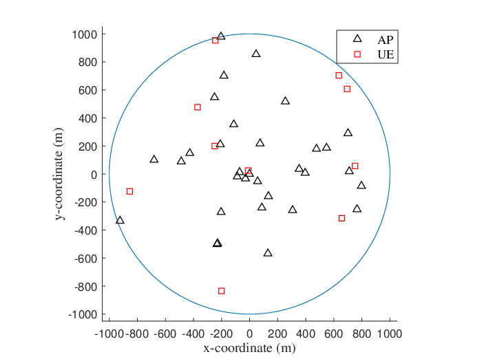
Fig. 2: A system topology with M=32M=32 APs and N=10N=10 UEs is used in numerical examples.

VII-A Simulation Parameters

A CFmMIMO-NOMA system including M=32M=32 APs and N=10N=10 UEs is considered as shown in Fig. I, where all APs and UEs are uniformly distributed within a circular region with a radius of 1 km. The large-scale fading of all channels is modeled as [6] βm,nl= 10PL⁡(dm,nl)+σs​h​z10\displaystyle\beta_{m,n_{l}}=\ 10^{\frac{{\rm{PL}}(d_{m,n_{l}})+\sigma_{sh}z}{10}}, ∀m∈ℳ\forall m\in\mathcal{M}, nl∈𝒩ln_{l}\in\mathcal{N}_{l}, where dm,nld_{m,n_{l}} is the distance from APm to UE nl{n_{l}}. The shadow fading is modeled as an RV zz, which follows 𝒞​𝒩​(0,1)\mathcal{CN}(0,1) with standard deviation σs​h\sigma_{sh} = 8 dB. The three-slope path loss model is considered as [6, 37, 29]

PL⁡(dm,nl)\displaystyle{\rm{PL}}(d_{m,n_{l}}) =−140.7−35​l​o​g10​(dm,nl)+20​a0​log10​(dm,nld0)+15​a1​log10​(dm,nld1),\displaystyle=-140.7-35{\rm{log}}_{10}(d_{m,n_{l}})+20a_{0}{\rm{log}}_{10}\Bigl(\frac{d_{m,n_{l}}}{d_{0}}\Bigr)+15a_{1}{\rm{log}}_{10}\Bigl(\frac{d_{m,n_{l}}}{d_{1}}\Bigr), (51)

where djd_{j}, with j={0,1}j=\left\{0,1\right\}, represents the reference distance and aj=max⁡{0,di−dm,nl|di−dm,nl|}a_{j}={{\rm{max}}\left\{0,\frac{d_{i}-d_{m,n_{l}}}{|d_{i}-d_{m,n_{l}}|}\right\}}. Note that PL⁡(dm,nl){\rm{PL}}(d_{m,n_{l}}) in (51) is measured in dB, while all distances are in km. Unless otherwise stated, other key parameters are shown in Table I, where all APs are assumed to have the same power budget [29, 6]. The used convex solver is SeDuMi [35] in the MATLAB environment.

VII-B Selection of the Number of Clusters L

TABLE II: Silhouette Score for CFmMIMO-NOMA and COmMIMO-NOMA.
Number of clusters LL 2 3 4 5 6 7 8 9
Silhouette Score CFmMIMO-NOMA 0.86 0.08 0.52 0.97 0.23 0.36 0.52 0.89
COmMIMO-NOMA 0.90 0.85 0.67 0.99 0.65 0.78 0.88 0.93

The performance of the k-means based UC algorithms is highly affected by the value of number of clusters LL [24, 25]. Thus, it is essential to investigate the particular feature of the UEs’ distribution in CFmMIMO-NOMA system to choose a proper number of clusters, such that the SSE is maximized. A reliable and precise approach to validate the optimal number of clusters LL is the silhouette score [38], which is the mean silhouette coefficient of all UEs. The silhouette coefficient of an UE is calculated as c−bmax⁡(c,b)\displaystyle\frac{c-b}{{\rm{max}}(c,b)}, where bb denotes the mean distance to other UEs in the same cluster (so-called the mean intra-cluster distance), and cc represents the mean distance to UEs of the next closest cluster which is the one that minimizes bb, excluding the UE’s own cluster (so-called mean nearest-cluster distance). The value of the silhouette coefficient ranges from -1 to +1. A coefficient close to +1 means that the UE is well matched to its own cluster and far from other clusters. A coefficient close to 0 indicates that the UE is near a cluster boundary, whereas a coefficient close to -1 implies that the UE is assigned to the wrong cluster. Table II shows the silhouette score versus the number of clusters LL. It is observed that the optimal number of clusters for this setting is L⋆=5L^{\star}=5.

In what follows, we set L=5L=5 to verify the performance analysis in Section VII-C and to evaluate the performance of the proposed algorithms in Section VII-D.

VII-C Numerical Results for the Performance Analysis

Refer to caption
Fig. 3: The SSE of CFmMIMO-NOMA versus the total power budget of all APs for the k-means, k-means++, and improved k-means++ algorithms.
Refer to caption
Fig. 4: The SSE of CFmMIMO-NOMA and COmMIMO-NOMA versus the total power budget of all APs.

We now investigate the performance of the two proposed unsupervised ML-based UC algorithms with fixed PA. The transmit power at each AP allocated to a specific UE follows the fixed PA scheme. Each AP allocates equal power to each cluster, and then, the fractional transmit PA [39] is used to allocate the power to a specific UE in each cluster based on the virtual channel gains presented in Section IV. As a benchmark, we also consider the COmMIMO-NOMA system, which is presented in Section VI.

Fig. 4 illustrates the SSE performance of CFmMIMO-NOMA versus the total power budget of all APs for the proposed UC algorithms. For comparison, the performance of the k-means algorithm is also plotted. It can be seen that the proposed UC algorithms significantly outperform the conventional k-means one. On the other hand, the improved k-means++ achieves the best SSE among all algorithms. This further confirms the importance of the effective initialization of centroids that improves the quality of the grouping process; otherwise, the use of NOMA becomes less efficient. Next, the SSE performance of the CFmMIMO-NOMA and COmMIMO-NOMA systems using the improved k-means++ algorithm versus the total power budget of all APs is shown in Fig. 4. We can observe that the performance of the CFmMIMO-NOMA system is better than that of COmMIMO-NOMA. This is attributed to the fact that CFmMIMO with many distributed APs brings the service antennas closer to UEs which not only reduces path losses but also provides higher degree of macro-diversity, compared to COmMIMO. Further, from Figs. 4 and 4, simulation results are well matched with the derived closed-form expressions of SSE in Section IV, verifying the correctness of our analytical results. In the following numerical results, unless otherwise specified, the improved k-means++ algorithm is used for UC.

VII-D Numerical Results for Optimal Power Allocation (Algorithm 4)

Refer to caption
Fig. 5: Convergence behavior of Algorithm 4 with different number of AP antennas, KK.

In Fig. 5, we evaluate the convergence speed of Algorithm 4 for CFmMIMO-NOMA and COmMIMO-NOMA with different values of KK. The proposed algorithm converges within three iterations and the convergence speed of both systems is not sensitive to the number of AP antennas, KK. As expected, the SSE is monotonically increasing after each iteration. Compared to the results in Figs. 4 and 4 with fixed PA at the power budget of 40 dBm, Algorithm 4 yields a significantly better performance in terms of SSE. The results demonstrate the effectiveness of the proposed algorithm to achieve the optimal SSE.
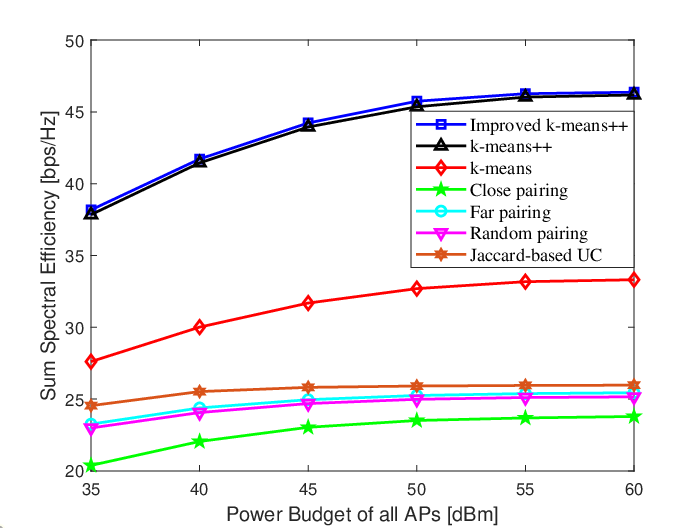
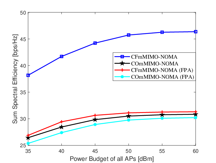
Refer to caption
Fig. 6: The SSE of different UC algorithms.
Refer to caption
Fig. 7: SSE of CFmMIMO-NOMA and COmMIMO-NOMA: with and without PA.

Fig. 7 shows the impact of the proposed k-means++ and improved k-means++ algorithms on the system performance of CFmMIMO-NOMA. For comparison, we also plot the SSE of the k-means (i.e., Algorithm 1) and the recently proposed UC approaches, including near pairing, far pairing, random pairing [16], and the Jaccard-based UC [17]. The main result observed from the figure is that the proposed unsupervised ML-based UC algorithms achieve better SSE performance compared to the baseline ones, and the performance gaps are wider when PmaxP_{\max} increases. This implies that the two proposed UC schemes are capable of exploiting UC more effectively, so that the SSE is remarkably enhanced. In Fig. 7, we demonstrate the benefit of optimizing PA for CFmMIMO-NOMA and COmMIMO-NOMA systems. The SSE of both systems is significantly enhanced with optimal PA compared to the fixed PA scheme. Hence, this shows the necessity of optimizing PA for both systems, especially for the CFmMIMO-NOMA system.

Refer to caption
Fig. 8: The effect of SIC performance coefficient on the SSE of CFmMIMO-NOMA and COmMIMO-NOMA systems.
Refer to caption
Fig. 9: The joint effect of the numbers of antennas KK and APs MM on the average SSE of different UC algorithms.

Next, the effect of the SIC performance coefficient ζnl\zeta_{{n}_{l}} on the SSE of CFmMIMO-NOMA and COmMIMO-NOMA is examined in Fig. 9. We note that ζnl=1\zeta_{{n}_{l}}=1 (ζnl=0\zeta_{{n}_{l}}=0) indicates no SIC (perfect SIC), while 0<ζnl<10<\zeta_{{n}_{l}}<1 means imperfect SIC. The system performance without NOMA/SIC is plotted. It is clear that the SSE of CFmMIMO-NOMA degrades when ζnl,∀nl\zeta_{{n}_{l}},\forall n_{l} increases. It implies that the SIC performance coefficient requires to be small enough to exploit the full potential of NOMA in CFmMIMO. Nevertheless, the SSE achieved by CFmMIMO-NOMA and COmMIMO-NOMA systems is much higher than their counterparts without NOMA/SIC.

Finally, we investigate the joint effect of the numbers of antennas KK and APs MM on the average SSE of different UC algorithms. We fix M​K=256MK=256 and select KK from the set K∈[8,16,32,64,128,256]K\in[8,16,32,64,128,256]. When K=256K=256, then M=1M=1, which represents COmMIMO-NOMA. From the figure, we see that the SSE first increases and then decreases when KK increases. This result reveals an interesting insight: for extremely small KK, the use of fpZF is less efficient in terms of canceling inter-cluster interference. However, the higher the value of KK, the lower the value of APs MM. This not only increases path losses, but also reduces the degree of macro-diversity. The results suggest that the optimal value of (M,K)(M,K) can improve the SSE of CFmMIMO-NOMA, e.g., (M,K)=(16,16)(M,K)=(16,16) for improved k-means++ and (M,K)=(32,8)(M,K)=(32,8) for k-means++ in this setting.

VIII Conclusion

In this paper, we have investigated downlink CFmMIMO-NOMA system, where two efficient unsupervised ML-based UC algorithms are developed to effectively cluster users into disjoint clusters. Using the fpZF precoding at APs, we have derived closed-form expressions for the SSE of CFmMIMO-NOMA, taking into account effects of intra-cluster pilot contamination, inter-cluster interference, and imperfect SIC. In addition, we have considered the problem of power allocation to maximize SSE. Since the formulated problem is intractable, we have developed a low-complexity iterative algorithm based on the IA framework for its solution. Numerical results have confirmed the effectiveness of the proposed UC algorithms, and show their superior performance compared to the baseline schemes. The proposed PA algorithm converges fast, and significantly outperforms CFmMIMO-NOMA without optimizing PA and COmMIMO-NOMA in terms of SSE.

Appendix A Proof of Lemma 1

1) Computation of |DSnl|2|\text{DS}_{n_{l}}|^{2}: By using (5) and (IV), the numerator in (23) is rewritten as

|DSnl|2=|𝔼{∑m∈ℳρnlmhm,nlH𝒘m,l}|2=|𝔼{∑m∈ℳρnlmh^m,nlH𝒘m,l}|2=(K−τp)(∑m∈ℳρnlm​γm,nl)2,\displaystyle|\text{DS}_{n_{l}}|^{2}=\Bigl|\mathbb{E}\Bigl\{\sum\limits_{m\in\mathcal{M}}\sqrt{\rho^{m}_{n_{l}}}\textbf{h}_{m,n_{l}}^{H}\boldsymbol{w}_{m,l}\Bigl\}\Bigl|^{2}=\Bigl|\mathbb{E}\Bigl\{\sum\limits_{m\in\mathcal{M}}\sqrt{\rho^{m}_{n_{l}}}\hat{\textbf{h}}_{m,n_{l}}^{H}\boldsymbol{w}_{m,l}\Bigl\}\Bigl|^{2}=(K-\tau_{p})\Bigl(\sum\limits_{m\in\mathcal{M}}\sqrt{\rho^{m}_{n_{l}}\gamma_{m,n_{l}}}\Bigl)^{2}, (52)

where the second equality is obtained due to the independence between the estimation error vector em,nl\textbf{e}_{m,n_{l}} and the channel estimate h^m,nl\hat{\textbf{h}}_{m,n_{l}}.

2) Computation of 𝔼​{|BUnl|2}\mathbb{E}\left\{|\text{BU}_{n_{l}}|^{2}\right\}: The first term of the denominator in (23) is reformulated as

𝔼​{|BUnl|2}\displaystyle\mathbb{E}\left\{|\text{BU}_{n_{l}}|^{2}\right\} =𝔼{|(∑m∈ℳρnlmhm,nlH𝒘m,l−𝔼{∑m∈ℳρnlmhm,nlH𝒘m,l})|2}\displaystyle=\mathbb{E}\Bigl\{\Bigl|\Bigl(\sum\limits_{m\in\mathcal{M}}\sqrt{\rho^{m}_{n_{l}}}\textbf{h}_{m,n_{l}}^{H}\boldsymbol{w}_{m,l}-\mathbb{E}\Bigl\{\sum\limits_{m\in\mathcal{M}}\sqrt{\rho^{m}_{n_{l}}}\textbf{h}_{m,n_{l}}^{H}\boldsymbol{w}_{m,l}\Bigl\}\Bigl)\Bigl|^{2}\Bigl\}
=𝔼{|∑m∈ℳρnlmhm,nlH𝒘m,l|2}−|𝔼{∑m∈ℳρnlmhm,nlH𝒘m,l}|2.\displaystyle=\mathbb{E}\Bigl\{\Bigl|\sum\limits_{m\in\mathcal{M}}\sqrt{\rho^{m}_{n_{l}}}\textbf{h}_{m,n_{l}}^{H}\boldsymbol{w}_{m,l}\Bigl|^{2}\Bigl\}-\Bigl|\mathbb{E}\Bigl\{\sum\limits_{m\in\mathcal{M}}\sqrt{\rho^{m}_{n_{l}}}\textbf{h}_{m,n_{l}}^{H}\boldsymbol{w}_{m,l}\Bigl\}\Bigl|^{2}. (53)

According to (5) and (IV), the first term in (A) is further derived as follows:

𝔼{|∑m∈ℳρnlmhm,nlH𝒘m,l|2}\displaystyle\mathbb{E}\Bigl\{\Bigl|\sum\limits_{m\in\mathcal{M}}\sqrt{\rho^{m}_{n_{l}}}\textbf{h}_{m,n_{l}}^{H}\boldsymbol{w}_{m,l}\Bigl|^{2}\Bigl\} =𝔼{|∑m∈ℳρnlmh^m,nlH𝒘m,l|2}+𝔼{|∑m∈ℳρnlmem,nlH𝒘m,l|2}\displaystyle=\mathbb{E}\Bigl\{\Bigl|\sum\limits_{m\in\mathcal{M}}\sqrt{\rho^{m}_{n_{l}}}\hat{\textbf{h}}_{m,n_{l}}^{H}\boldsymbol{w}_{m,l}\Bigl|^{2}\Bigl\}+\mathbb{E}\Bigl\{\Bigl|\sum\limits_{m\in\mathcal{M}}\sqrt{\rho^{m}_{n_{l}}}\textbf{e}_{m,n_{l}}^{H}\boldsymbol{w}_{m,l}\Bigl|^{2}\Bigl\}
=(K−τp)(∑m∈ℳρnlm​γm,nl)2+∑m∈ℳρnlm(βm,nl−γm,nl).\displaystyle=(K-\tau_{p})\Bigl(\sum\limits_{m\in\mathcal{M}}\sqrt{\rho^{m}_{n_{l}}\gamma_{m,n_{l}}}\Bigl)^{2}+\sum\limits_{m\in\mathcal{M}}\rho^{m}_{n_{l}}\Bigl(\beta_{m,n_{l}}-\gamma_{m,n_{l}}\Bigl). (54)

Substituting (52) and (A) into (A), (A) can be rewritten as

𝔼{|BUnl|2}\displaystyle\mathbb{E}\Bigl\{|\text{BU}_{n_{l}}|^{2}\Bigl\} =(K−τp)(∑m∈ℳρnlm​γm,nl)2+∑m∈ℳρnlm(βm,nl−γm,nl)\displaystyle=(K-\tau_{p})\Bigl(\sum\limits_{m\in\mathcal{M}}\sqrt{\rho^{m}_{n_{l}}\gamma_{m,n_{l}}}\Bigl)^{2}+\sum\limits_{m\in\mathcal{M}}\rho^{m}_{n_{l}}\left(\beta_{m,n_{l}}-\gamma_{m,n_{l}}\right)
−(K−τp)(∑m∈ℳρnlm​γm,nl)2\displaystyle-(K-\tau_{p})\Bigl(\sum\limits_{m\in\mathcal{M}}\sqrt{\rho^{m}_{n_{l}}\gamma_{m,n_{l}}}\Bigl)^{2}
=∑m∈ℳρnlm​(βm,nl−γm,nl).\displaystyle=\sum\limits_{m\in\mathcal{M}}\rho^{m}_{n_{l}}\left(\beta_{m,n_{l}}-\gamma_{m,n_{l}}\right). (55)

3) Computation of ∑n′l=1nl−1𝔼⁡{|ICInl|2}\sum\limits_{{n^{\prime}}_{l}=1}^{n_{l}-1}\mathbb{E}\left\{|\text{ICI}_{n_{l}}|^{2}\right\}: Based on (A), the second term of the denominator in (23) is computed as

∑n′l=1nl−1𝔼⁡{|ICInl|2}\displaystyle\sum\limits_{{n^{\prime}}_{l}=1}^{n_{l}-1}\mathbb{E}\left\{|\text{ICI}_{n_{l}}|^{2}\right\} =∑n′l=1nl−1𝔼{|∑m∈ℳρn′lmhm,nlH𝒘m,l|2}\displaystyle=\sum\limits_{{n^{\prime}}_{l}=1}^{n_{l}-1}\mathbb{E}\Bigl\{\Bigl|\sum\limits_{m\in\mathcal{M}}\sqrt{\rho^{m}_{{n^{\prime}}_{l}}}\textbf{h}_{m,n_{l}}^{H}\boldsymbol{w}_{m,l}\Bigl|^{2}\Bigl\}
=∑n′l=1nl−1(K−τp)(∑m∈ℳρn′lm​γm,nl)2+∑n′l=1nl−1∑m∈ℳρn′lm(βm,nl−γm,nl).\displaystyle=\sum\limits_{{n^{\prime}}_{l}=1}^{n_{l}-1}(K-\tau_{p})\Bigl(\sum\limits_{m\in\mathcal{M}}\sqrt{\rho^{m}_{{n^{\prime}}_{l}}\gamma_{m,n_{l}}}\Bigl)^{2}+\sum\limits_{{n^{\prime}}_{l}=1}^{n_{l}-1}\sum\limits_{m\in\mathcal{M}}\rho^{m}_{{n^{\prime}}_{l}}\left(\beta_{m,n_{l}}-\gamma_{m,n_{l}}\right). (56)

4) Computation of ∑n′′l=nl+1Nl𝔼⁡{|RICInl|2}\sum\limits_{{n^{\prime\prime}}_{l}=n_{l}+1}^{N_{l}}\mathbb{E}\left\{|\text{RICI}_{n_{l}}|^{2}\right\}: According to (A), the third term of the denominator in (23) is rewritten as

∑n′′l=nl+1Nl𝔼⁡{|RICInl|2}\displaystyle\sum\limits_{{n^{\prime\prime}}_{l}=n_{l}+1}^{N_{l}}\mathbb{E}\left\{|\text{RICI}_{n_{l}}|^{2}\right\} =∑n′′l=nl+1Nl𝔼{|ζnl∑m∈ℳρn′′lmhm,nlH𝒘m,lxn′′l|2}\displaystyle=\sum\limits_{{n^{\prime\prime}}_{l}=n_{l}+1}^{N_{l}}\mathbb{E}\Bigl\{\Bigl|\sqrt{\zeta_{{n}_{l}}}\sum\limits_{m\in\mathcal{M}}\sqrt{\rho^{m}_{{n^{\prime\prime}}_{l}}}\textbf{h}_{m,n_{l}}^{H}\boldsymbol{w}_{m,l}x_{{n^{\prime\prime}}_{l}}\Bigl|^{2}\Bigl\}
=∑n′′l=nl+1Nlζnl(K−τp)(∑m∈ℳρn′′lm​γm,nl)2\displaystyle=\sum\limits_{{n^{\prime\prime}}_{l}=n_{l}+1}^{N_{l}}\zeta_{{n}_{l}}(K-\tau_{p})\Bigl(\sum\limits_{m\in\mathcal{M}}\sqrt{\rho^{m}_{{n^{\prime\prime}}_{l}}\gamma_{m,n_{l}}}\Bigl)^{2}
+∑n′′l=nl+1Nl∑m∈ℳζnlρn′′lm(βm,nl−γm,nl).\displaystyle+\sum\limits_{{n^{\prime\prime}}_{l}=n_{l}+1}^{N_{l}}\sum\limits_{m\in\mathcal{M}}\zeta_{{n}_{l}}\rho^{m}_{{n^{\prime\prime}}_{l}}\left(\beta_{m,n_{l}}-\gamma_{m,n_{l}}\right). (57)

5) Computation of 𝔼​{|UInl|2}\mathbb{E}\left\{|\text{UI}_{n_{l}}|^{2}\right\}: From (A), the fourth term of the denominator in (23) is shown as follows:

𝔼​{|UInl|2}\displaystyle\mathbb{E}\left\{|\text{UI}_{n_{l}}|^{2}\right\} =∑l′∈ℒ∖{l}∑nl′=1Nl′𝔼{|∑m∈ℳρnl′mhm,nlH𝒘m,l′|2}\displaystyle=\sum\limits_{{l^{\prime}}\in\mathcal{L}\setminus\{l\}}\sum\limits_{n_{l^{\prime}}=1}^{N_{l^{\prime}}}\mathbb{E}\Bigl\{\Bigl|\sum\limits_{m\in\mathcal{M}}\sqrt{\rho^{m}_{{n}_{l^{\prime}}}}\textbf{h}_{m,n_{l}}^{H}\boldsymbol{w}_{m,{l^{\prime}}}\Bigl|^{2}\Bigl\}
=∑l′∈ℒ∖{l}∑nl′=1Nl′𝔼{|∑m∈ℳρnl′mem,nlH𝒘m,l′|2}\displaystyle=\sum\limits_{{l^{\prime}}\in\mathcal{L}\setminus\{l\}}\sum\limits_{n_{l^{\prime}}=1}^{N_{l^{\prime}}}\mathbb{E}\Bigl\{\Bigl|\sum\limits_{m\in\mathcal{M}}\sqrt{\rho^{m}_{{n}_{l^{\prime}}}}\textbf{e}_{m,n_{l}}^{H}\boldsymbol{w}_{m,{l^{\prime}}}\Bigl|^{2}\Bigl\}
=∑l′∈ℒ∖{l}∑nl′=1Nl′∑m∈ℳρnl′m​(βm,nl−γm,nl),\displaystyle=\sum\limits_{{l^{\prime}}\in\mathcal{L}\setminus\{l\}}\sum\limits_{n_{l^{\prime}}=1}^{N_{l^{\prime}}}\sum\limits_{m\in\mathcal{M}}\rho^{m}_{{n}_{l^{\prime}}}\left(\beta_{m,n_{l}}-\gamma_{m,n_{l}}\right), (58)

where the second equality in (A) is obtained due to the property of the fpZF precoding.

Finally, by substituting (52), (A), (A), (A), and (A) into (23), SINRnlnl\text{SINR}^{n_{l}}_{n_{l}} is obtained as in (27). Following the similar steps for deriving SINRnlnl\text{SINR}^{n_{l}}_{n_{l}}, SINRn′lnl\text{SINR}^{n_{l}}_{{n^{\prime}}_{l}} can be easily derived as in (28).

Appendix B Proof of Proposition 1

By contradiction and IA principles, we can easily prove that constraints (33aa)-(33c), (34), (35a)-(38a) and (41d) must hold with equality at optimum. Let us define ℱ⁡(φnl)≜ln⁡(1+φnl)\mathcal{F}(\varphi_{n_{l}})\triangleq\ln(1+\varphi_{n_{l}}). From (40), we have

ℱ⁡(φnl)≥ℱ(κ)​(φ(κ),φ¯nl),\mathcal{F}(\varphi_{n_{l}})\geq\mathcal{F}^{(\kappa)}(\varphi^{(\kappa)},\bar{\varphi}_{n_{l}}), (59)

and

ℱ⁡(φnl(κ))=ℱ(κ)​(φ(κ),φ¯nl).\mathcal{F}(\varphi_{n_{l}}^{(\kappa)})=\mathcal{F}^{(\kappa)}(\varphi^{(\kappa)},\bar{\varphi}_{n_{l}}). (60)

Thus, it is true that

ℱ⁡(φnl(κ))≥ℱ(κ−1)​(φ(κ),φ¯nl)≥ℱ(κ−1)​(φ(κ−1),φ¯nl)=ℱ⁡(φnl(κ−1)).\mathcal{F}(\varphi_{n_{l}}^{(\kappa)})\geq\mathcal{F}^{(\kappa-1)}(\varphi^{(\kappa)},\bar{\varphi}_{n_{l}})\geq\mathcal{F}^{(\kappa-1)}(\varphi^{(\kappa-1)},\bar{\varphi}_{n_{l}})=\mathcal{F}(\varphi_{n_{l}}^{(\kappa-1)}). (61)

These results imply that (ϖ(κ),𝜽(κ),𝝋(κ))(\boldsymbol{\varpi}^{(\kappa)},{\boldsymbol{\theta}}^{(\kappa)},\boldsymbol{\varphi}^{(\kappa)}) is an improved solution to problem (41), compared to (ϖ(κ−1)CLOSE,(\boldsymbol{\varpi}^{(\kappa-1)}, OPEN𝜽(κ−1),𝝋(κ−1)){\boldsymbol{\theta}}^{(\kappa-1)},\boldsymbol{\varphi}^{(\kappa-1)}). By [27, Theorem 1], the sequence {ϖ(κ),𝜽(κ),𝝋(κ)}\{\boldsymbol{\varpi}^{(\kappa)},{\boldsymbol{\theta}}^{(\kappa)},\boldsymbol{\varphi}^{(\kappa)}\} converges to at least local optima which satisfy the KKT conditions. As a result, the objective value of problem (41) is monotonically increasing, i.e., (1−τpτc)​∑l∈ℒ∑nl∈𝒩lrnl(κ)≥(1−τpτc)​∑l∈ℒ∑nl∈𝒩lrnl(κ−1)\bigl(1-\frac{\tau_{p}}{\tau_{c}}\bigr)\sum\limits_{l\in\mathcal{L}}\sum\limits_{n_{l}\in\mathcal{N}_{l}}r_{n_{l}}^{(\kappa)}\geq\bigl(1-\frac{\tau_{p}}{\tau_{c}}\bigr)\sum\limits_{l\in\mathcal{L}}\sum\limits_{n_{l}\in\mathcal{N}_{l}}r_{n_{l}}^{(\kappa-1)}. In addition, the sequence of the objective values is upper bounded due to power constraints (39c), which completes the proof.

References

  • [1] Iot-analytics.com, State of the IoT 2018: Number of IoT devices now at 7B – Market accelerating, Aug. 2018. [Online]. Available: https://iot-analytics.com/state-of-the-iot-update-q1-q2-2018-number-of-iot-devices-now-7b
  • [2] Cisco Visual Networking Index: Global Mobile Data Traffic Forecast Update, 2016-2021, Mar. 2017. [Online]. Available: https://www.cisco.com/c/en/us/solutions/collateral/service-provider/visual-networking-index-vni/mobile-white-paper-c11-520862.html
  • [3] S. M. R. Islam, N. Avazov, O. A. Dobre, and K.-S. Kwak, “Power-domain non-orthogonal multiple access (NOMA) in 5G systems: Potentials and challenges,” IEEE Commun. Surveys Tuts., vol. 19, no. 2, pp. 721–742, 2nd Quart. 2017.
  • [4] V.-D. Nguyen, H. D. Tuan, T. Q. Duong, H. V. Poor, and O.-S. Shin, “Precoder design for signal superposition in MIMO-NOMA multicell networks,” IEEE J. Select. Areas Commun., vol. 35, no. 12, pp. 2681–2695, Dec. 2017.
  • [5] H. V. Nguyen, V.-D. Nguyen, O. A. Dobre, D. N. Nguyen, E. Dutkiewicz, and O.-S. Shin, “Joint power control and user association for NOMA-based full-duplex systems,” IEEE Trans. Commun., vol. 67, no. 11, pp. 8037–8055, Nov. 2019.
  • [6] H. Q. Ngo, A. Ashikhmin, H. Yang, E. G. Larsson, and T. L. Marzetta, “Cell-free massive MIMO versus small cells,” IEEE Trans. Wireless Commun., vol. 16, no. 3, pp. 1834–1850, Mar. 2017.
  • [7] E. Nayebi, A. Ashikhmin, T. L. Marzetta, H. Yang, and B. D. Rao, “Precoding and power optimization in cell-free massive MIMO systems,” IEEE Trans. Wireless Commun., vol. 16, no. 7, pp. 4445–4459, July 2017.
  • [8] M. Bashar, K. Cumanan, A. G. Burr, M. Debbah, and H. Q. Ngo, “On the uplink max–min SINR of cell-free massive MIMO systems,” IEEE Trans. Wireless Commun., vol. 18, no. 4, pp. 2021–2036, Apr. 2019.
  • [9] H. Q. Ngo, L.-N. Tran, T. Q. Duong, M. Matthaiou, and E. G. Larsson, “On the total energy efficiency of cell-free massive MIMO,” IEEE Trans. Green Commun. Netw., vol. 2, no. 1, pp. 25–39, Mar. 2018.
  • [10] Z. Chen and E. Björnson, “Channel hardening and favorable propagation in cell-free massive MIMO with stochastic geometry,” IEEE Trans. Commun., vol. 66, no. 11, pp. 5205–5219, Nov. 2018.
  • [11] X. Chen, D. W. K. Ng, W. Yu, E. G. Larsson, N. Al-Dhahir, and R. Schober, “Massive access for 5G and beyond,” Feb. 2020. [Online]. Available: https://arxiv.org/abs/2002.03491
  • [12] Y. Li and G. A. A. Baduge, “NOMA-aided cell-free massive MIMO systems,” IEEE Wireless Commun. Lett., vol. 7, no. 6, pp. 950–953, Dec. 2018.
  • [13] Y. Zhang, H. Cao, M. Zhou, and L. Yang, “Spectral efficiency maximization for uplink cell-free massive MIMO-NOMA networks,” in 2019 IEEE Inter. Conf. Commun. Works. (ICC Workshops), May 2019, pp. 1–6.
  • [14] F. Rezaei, C. Tellambura, A. A. Tadaion, and A. R. Heidarpour, “Rate analysis of cell-free massive MIMO-NOMA with three linear precoders,” IEEE Trans. Commun., vol. 68, no. 6, pp. 3480–3494, June 2020.
  • [15] S. M. R. Islam, M. Zeng, O. A. Dobre, and K.-S. Kwak, “Resource allocation for downlink NOMA systems: Key techniques and open issues,” IEEE Wireless Commun., vol. 25, no. 2, pp. 40–47, Apr. 2018.
  • [16] M. Bashar, K. Cumanan, A. G. Burr, H. Q. Ngo, L. Hanzo, and P. Xiao, “On the performance of cell-free massive MIMO relying on adaptive NOMA/OMA mode-switching,” IEEE Trans. Commun., vol. 68, no. 2, pp. 792–810, Feb. 2020.
  • [17] F. Rezaei, A. R. Heidarpour, C. Tellambura, and A. A. Tadaion, “Underlaid spectrum sharing for cell-free massive MIMO-NOMA,” IEEE Commun. Lett., vol. 24, no. 4, pp. 907–911, Apr. 2020.
  • [18] R. He, Q. Li, B. Ai, Y. L.-A. Geng, A. F. Molisch, V. Kristem, Z. Zhong, and J. Yu, “A kernel-power-density-based algorithm for channel multipath components clustering,” IEEE Trans. Wireless Commun., vol. 16, no. 11, pp. 7138–7151, Nov. 2017.
  • [19] X. Xie, Z. Zhang, H. Jiang, J. Dang, and L. Wu, “Cluster-based geometrical dynamic stochastic model for MIMO scattering channels,” in Proc. Inter. Conf. Wireless Commun. and Signal Process. (WCSP), Oct. 2017, pp. 1–5.
  • [20] Y. Wang, A. Liu, X. Xia, and K. Xu, “Exploiting the clustered sparsity for channel estimation in hybrid analog-digital massive MIMO systems,” IEEE Access, vol. 7, pp. 4989–5000, Dec. 2018.
  • [21] A. B. Rozario and M. F. Hossain, “An architecture for M2M communications over cellular networks using clustering and hybrid TDMA-NOMA,” in Proc. Inter. Conf. Infor. and Commun. Tech. (ICoICT), May 2018, pp. 18–23.
  • [22] A. K. Jain, “Data clustering: 50 years beyond k-means,” Pattern Recognition Lett., vol. 31, no. 8, pp. 651–666, June 2010.
  • [23] E. Cabrera and R. Vesilo, “An enhanced k-means clustering algorithm with non-orthogonal multiple access (NOMA) for MMC networks,” in Proc. Inter. Telecommun Net. and App. Conf. (ITNAC), Nov. 2018, pp. 1–8.
  • [24] J. Cui, Z. Ding, P. Fan, and N. Al-Dhahir, “Unsupervised machine learning-based user clustering in millimeter-wave-NOMA systems,” IEEE Trans. Wireless Commun., vol. 17, no. 11, pp. 7425–7440, Sep. 2018.
  • [25] F. Riera-Palou, G. Femenias, A. G. Armada, and A. Pérez-Neira, “Clustered cell-free massive MIMO,” in Proc. IEEE Globecom Workshops (GC Wkshps), Dec. 2018, pp. 1–6.
  • [26] M. Morales-Céspedes, O. A. Dobre, and A. García-Armada, “Semi-blind interference aligned NOMA for downlink MU-MISO systems,” IEEE Trans. Commun., vol. 68, no. 3, pp. 1852–1865, Mar. 2020.
  • [27] B. R. Marks and G. P. Wright, “A general inner approximation algorithm for nonconvex mathematical programs,” Oper. Res., vol. 26, no. 4, pp. 681–683, July-Aug. 1978.
  • [28] G. Interdonato, M. Karlsson, E. Bjornson, and E. G. Larsson, “Downlink spectral efficiency of cell-free massive MIMO with full-pilot zero-forcing,” in IEEE Global Conf. Signal and Infor. Process. (GlobalSIP), Nov. 2018, pp. 1003–1007.
  • [29] H. V. Nguyen, V.-D. Nguyen, O. A. Dobre, S. K. Sharma, S. Chatzinotas, B. Ottersten, and O.-S. Shin, “On the spectral and energy efficiencies of full-duplex cell-free massive MIMO,” IEEE J. Select. Areas Commun., pp. 1–1, June 2020.
  • [30] D. Arthur and S. Vassilvitskii, “K-means++: The advantages of careful seeding,” in Proc. Symp. Discrete Algorithms, Jan. 2007, pp. 1027–1035.
  • [31] P. Fränti and S. Sieranoja, “How much can k-means be improved by using better initialization and repeats?” Pattern Recognit., vol. 93, pp. 95–112, Sep. 2019.
  • [32] O. Bachem, M. Lucic, S. H. Hassani, and A. Krause, “Approximate k-means++ in sublinear time,” in Proc. 30th AAAI Conf. Artif. Intell., Feb. 2016, pp. 1459–1467.
  • [33] A. M. Tulino and S. Verdú, “Random matrix theory and wireless communications,” Commun. Inf. Theory, vol. 1, no. 1, pp. 1–182, June 2004.
  • [34] A. Beck, A. Ben-Tal, and L. Tetruashvili, “A sequential parametric convex approximation method with applications to nonconvex truss topology design problems,” J. Global Optim., vol. 47, no. 1, pp. 29–51, May 2010.
  • [35] J. F. Sturm, “Using sedumi 1.02, a MATLAB toolbox for optimization over symmetric cones,” Optimiz. Methods and Softw., vol. 11-12, pp. 625–653, Sep. 1999.
  • [36] “I. MOSEK aps,” 2014. [Online]. Available: http://www.mosek.com
  • [37] A. Tang, J. Sun, and K. Gong, “Mobile propagation loss with a low base station antenna for NLOS street microcells in urban area,” in Proc. IEEE Veh. Tech. Conf. (VTC Spring), May 2001, pp. 333–336.
  • [38] A. Geron, “Hands-on machine learning with scikit-learn and tensorflow: Concepts, tools, and techniques to build intelligent systems,” O’Reilly Media Inc., pp. 1–484, Sep. 2019.
  • [39] A. Benjebbour, A. Li, Y. Kishiyama, H. Jiang, and T. Nakamura, “System-level performance of downlink NOMA combined with SUMIMO for future LTE enhancements,” in Proc. IEEE Globecom Workshops (GC Wkshps), Dec. 2014, pp. 706–710.