Assessing Uncertainties in the Predicted Very-High-Energy Flux of Globular Clusters in the Cherenkov Telescope Array Era2020Assessing Uncertainties in the Predicted Very-High-Energy Flux of Globular Clusters in the Cherenkov Telescope Array Era—-References

Venter & Kopp 2015 applied a leptonic GC model to the population of clusters mentioned in Abramowski et al. 2013 to predict the live-time-averaged (stacked) flux and compare it to the H.E.S.S. stacking upper limits. They used fixed (best-guess) model parameters as noted in their Table 1, and used the inferred values from Abdo et al. 2010 for $N_{\rm MSP}$ where possible, and $N_{\star}$ values from Lang 1993, and obtained distances $d$ and structural parameters³³ 3 http://gclusters.altervista.org/index.php $r_{\rm c}$, $r_{\rm hm}$, and $r_{\rm t}$ from Harris 1996. Typical values of $\eta\sim 0.01$ (Venter & de Jager 2005), $N_{\rm MSP}\sim 25$, and $\langle\dot{E}\rangle\sim 2\times 10^{34}\,{\rm erg\,s^{-1}}$ led to typical values of $Q_{0}\sim 10^{33-34}\,{\rm erg^{-1}s^{-1}}$ for the source strength (see Equations [1] and [2]). They also used $B=5\mu G$ and $\Gamma=2.0$ throughout, and assumed optical photons from the stellar population embedded in the GC plus cosmic microwave background (CMB) photons as target fields for their IC calculation (assuming an average stellar temperature of $\langle T\rangle=4\,500$ K). They found that none of the predicted single-cluster spectra violated the H.E.S.S. TeV upper limits for individual sources. Their averaged flux furthermore satisfied the stringent stacking upper limits. However, they noted that different choices of parameters led to average fluxes that in some cases may exceed these limits. That is why we refine their calculation in this paper, now also including an estimation of uncertainties on the predicted VHE fluxes.

In this Section, we describe the method we employ for modelling the IC $\gamma$-ray flux expected from the 15 Galactic GCs observed by H.E.S.S. We follow the method of Venter & de Jager 2008 where they used a Monte Carlo technique to model the pulsed CR $\gamma$-ray flux and associated uncertainties expected from $100$ MSPs hosted by a GC. Their calculated CR flux was randomised over the magnetic inclination ($\alpha$) and observer ($\zeta$) angles that are usually estimated from radio polarisation measurements involving the rotating vector model (Manchester & Johnston 1995), as well as taking into account the fixed, pulsar-specific parameters such as period $P$ and period derivative $\dot{P}$ (or $\dot{E}$) of each MSP member. In our case, we use the same method to calculate the single-GC and stacked integral VHE flux of 15 GCs (Abramowski et al. 2013), with uncertainties due to the uncertainty in model parameters. We do this by randomising over seven free parameters as mentioned in Section 2: $B$, $\Gamma$, $N_{*}$, $d$, $\eta$, $\dot{E}$, and $N_{\rm MSP}$, in addition to fixing the structural and diffusion coefficient parameters as noted above.

We first apply the model of Kopp et al. 2013 to the population of clusters to obtain the differential spectrum (Section 2) for different parameter combinations, initially setting $Q_{0}=1$ and only using four free parameters ($B$, $\Gamma$, $N_{*}$, and $d$). We then calculate the integral flux using Equation (3) and obtain a spread of fluxes, based on the range of values we picked for these four parameters. To indicate the build-up of a smooth flux distribution, we use the four free parameters for illustration (for the full modeling, we use seven). Figure 2 thus indicates how a distribution of $\log_{10}$ of the integral flux becomes smooth as we increase the resolution at which each of four free parameters is sampled. A finer grid thus lead to a smoother distribution of fluxes.

Second, we indicate convergence of the flux distribution with an increase of the number of trials, again for four free model parameters. That is, we calculate the integral flux for $N_{t}$ trials (each trial corresponding to a different parameter combination on a pre-defined grid), obtaining convergence as $N_{\rm t}$ gets close to or exceeds the number of unique combinations ($N_{\rm comb}$) of the four free parameters. Thus, we reproduce the last panel of Figure 2 to indicate convergence in Figure 2. We note that undersampling will not give a smooth flux distribution, but oversampling will lead to convergence.

We thirdly check for the convergence of the source strength parameter $Q_{0}$ (see Figure 3) via two methods, using 47 Tucanae as an example. For the first method, we pick values of four relevant (different) parameters on a specified grid: $\eta\in[0.005,0.08]$ in steps of 0.005, $\log_{10}\langle\dot{E}\rangle\in[33.7,34.7]$ in steps of $0.05$, $N_{\rm MSP}\in[5,150]$ in steps of 1, and $\Gamma\in[1.7,2.9]$ in steps of $0.1$. For the second method, we randomise over the same four parameters $\eta$, $\log\dot{E}$, $N_{\rm MSP}$, and $\Gamma$, for fixed $E_{\rm e,min}=0.1\,{\rm TeV}$ and $E_{\rm e,max}=100\,{\rm TeV}$, within the parameter ranges given above (but not on a fixed grid). We conduct $N_{\rm t}=10^{6}$ trials in both cases. The two different approaches yield very similar results, which also correspond to the values found by Kopp et al. 2013 as well as to the calculation by Venter & Kopp 2015, with the two peaks in the histogram only slightly shifted with respect to each other. Thus, sampling on a grid vs. randomly picking parameter values does not make too much of a difference in terms of the distribution of $Q_{0}$.

We lastly perform nested loops over the seven free model parameters to calculate $Q_{0}(\Gamma,\eta,\langle\dot{E}\rangle,N_{\rm MSP})\neq 1$, and multiply the correct flux, pre-calculated for $Q_{0}=1$ and depending only on $B,\Gamma,d$, and $N_{*}$, by the actual value of $Q_{0}$ to obtain the final differential and integral fluxes in observational units (see Equation [1] and the final panel of Figure 4 for the case of 47 Tucanae). The spread in flux reflects the uncertainty in model parameters. We use the observational threshold energy $E_{\rm th}$ associated with a particular cluster to calculate $F(>E_{\rm th})$. In Figure 4, we randomly sample integral fluxes for a different total number of trials $N_{\rm t}$ from the grid of pre-calculated fluxes to show convergence as $N_{\rm t}\rightarrow N_{\rm comb}$.

MAGIC has recently published differential flux upper limits for M15 (Acciari et al. 2019; see Section 4.2 for details on the source and VHE data). We applied the model of Kopp et al. 2013 to M15 to obtain the differential fluxes for each combination of seven free model parameters (see Section 2). Next, we calculated the final differential flux as described in Section 3.1.

We again use the method of Venter & de Jager 2008 to estimate the uncertainty in the differential flux of M15 at 13 different observer-defined energy bins (Acciari et al. 2019). Specifically, we logarithmically interpolate model fluxes to obtain predictions at the specified observational energies associated with the upper limits. Our parameter grid for M15 was chosen as follows: $B\in[1,\,3,\,5,\,7,\,9]\,\mu G$, injection spectral index $\Gamma\in[1.7,\,2.0,\,2.3,\,2.6,\,2.9]$, $N_{*}\in[2.05,\,2.90,\,4.10,\,5.80,\,8.20]\times 10^{5}$, $d\in[5.20,\,7.35,\,10.4\,14.7,\,20.8]\,{\rm kpc}$, $\eta\in[0.003,0.063]$ with steps of $0.005$, $\log_{10}\langle\dot{E}\rangle\in[33.7,34.7]$ with steps of $0.05$, and the number of MSPs $N_{\rm MSP}\in[8,24]$, in steps of $1$. In the case of $\omega$ Cen, we used the same $B$ and $\Gamma$ range as for M15, but $N_{*}\in[0.5,\,0.7,\,1.0,\,1.4,\,2.0]\times 10^{6}$, $d\in[2.6,\,3.7,\,5.2,\,7.6,\,10.5]\,{\rm kpc}$, $\eta\in[0.005,0.055]$, $\log_{10}\langle\dot{E}\rangle\in[33.9,34.9]$ in steps of $0.05$, and $N_{\rm MSP}\in[5,299]$ in steps of 1. We conducted a maximum of $N_{\rm t}=10^{7}$ trials, with $N_{\rm comb}=2.9\times 10^{6}$ for M15 and $N_{\rm comb}=7.4\times 10^{6}$ for $\omega$ Cen, respectively (cf. Figure 5, where the value of $N_{t}$ is indicated in each panel).

To obtain a sample of GCs suited for the study by H.E.S.S., Abramowski et al. 2013 selected a population of clusters based on the GC catalog of Harris 2010 from which all the basic parameters such as position, $d$, $r_{\rm c}$, and central luminosity density $\rho_{0}$ have been taken. Abramowski et al. 2013 furthermore applied different cuts on the target and observation run lists:
1. GC $|{\rm Galactic\,latitude}|\geq 1.0^{\circ}$. This cut was done to conservatively exclude GCs towards the direction of the Galactic Plane to avoid faint emission from unresolved sources, diffuse emission, and also chance coincidences with unrelated sources.
2. Standard quality selection criteria were applied, with the telescopes pointed $<2.0^{\circ}$ offset from the GC position.
3. A selected GC had to have at least $20$ available runs passing the cut describe in point $2.$ to ensure a reasonably long exposure on these potentially faint sources.

In order to compare our model predictions with the H.E.S.S. flux upper limits $F_{\rm UL}$, we have to characterise the mean predicted flux plus its uncertainty⁴⁴ 4 We note that it is common in certain statistical contexts to use the $2^{\rm nd}$ quartile (median) as an indication of an average value, and the $1^{\rm st}$ and $3^{\rm rd}$ quartiles ($25^{\rm th}$ and $75^{\rm th}$ percentiles) as indications of uncertainty or the spread of values around the median, as is done in box plots. However, we opt to use the median and the $16^{\rm th}$ and $84^{\rm th}$ percentiles to estimate the average and uncertainty in model flux (in analogy to what is typical for a normal distribution of values), as is commonly done in certain physics contexts, given the fact that our flux distributions appear to be approximately log-normal. Our main conclusion, that there are large uncertainties on the median model fluxes due to uncertainty on model parameters, is not affected by this choice of convention. First, we obtain the median flux $F_{\mu}$ ($50^{\rm th}$ percentile) for each cluster, as well as the $16^{\rm th}$ and $84^{\rm th}$ percentile, as shown in Figure 6 and listed in Table 1. We calculate $\sigma_{16}=\mu-F_{16}$ and $\sigma_{84}=F_{84}-\mu$ and also express them as percentages: $100\sigma_{16}/\mu$ and $100\sigma_{84}/\mu$, with $F_{16}$ and $F_{84}$ being the $16^{\rm th}$ and $84^{\rm th}$ percentiles. We also calculate the geometric mean of the flux $\bar{F}_{\rm G}$ (since we want to be insensitive to outliers), as well as the standard deviation $\sigma$ of this flux, noting that the geometric mean is equal to the antilog of the arithmetic mean of the log of fluxes. We finally list the ratios $F_{\mu}/F_{\rm UL}$ as well as $\bar{F}_{\rm G}/F_{\mu}$, indicating that the median is usually below the upper limit, except for Djorg 2 and the stacking upper limit, and that $F_{\mu}\approx\bar{F}_{\rm G}$.

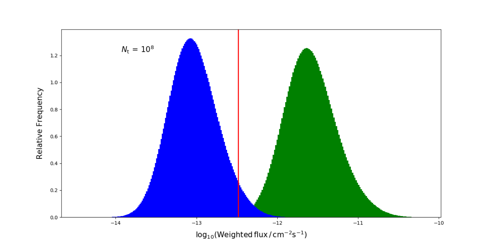
In Figure 7 we show the distribution of the $\log_{10}$ of weighted (stacked) flux for all GCs. We plot the weighted flux as a function of $N_{\rm t}$ for all 15 GCs. We use $E_{\rm th}=0.23$ TeV and calculate the weighted flux as

where $i$ represents a specific GC, $\tau_{i}$ is the live time (acceptance-corrected observational time passing quality cuts) for each GC, and $\tau_{\rm tot}$ is the total live time. The median and geometric mean of this quantity are listed in the bottom row of Table 1, in column 4 and 8, respectively, for comparison to the stacked upper limit published by H.E.S.S. as listed in column 3. The first set (range) of parameter combinations used for the green histograms in Figure 7 is as follows: $d_{\rm cluster}\in[\frac{d}{2},\frac{d}{\sqrt{2}},d,\sqrt{2}d,2d]$, $N_{*}\in[\frac{N}{2},\frac{N_{*}}{\sqrt{2}},N_{*},\sqrt{2}N_{*},2N_{*}]$ (see Venter & Kopp 2015 for values of $d$ and $N_{*}$). We used $B\in[1,9]$ in steps of 2, $\Gamma\in[1.7,2.9]$ with steps of 0.3, $\eta\in[0.005,0.08]$ in steps of 0.0075, $\log_{10}\langle\dot{E}\rangle\in[33.7,34.7]$ in steps of 0.1, and $N_{\rm MSP}\in[5,150]$ in steps of 10. Although somewhat arbitrary, these were chosen to be an example set of reasonable (best-guess) parameter values. However, we see from Table 1 that for this initial choice, the median stacked flux exceeds the upper limit by a factor of 7.6. We therefore considered a second parameter set, associated with the blue histograms of weighted flux for 15 GCs in Figure 7: $\eta\in[0.003,0.03]$ in steps of 0.003, $\log_{10}\langle\dot{E}\rangle\in[33,34]$ in steps of 0.1, and $N_{\rm MSP}\in[5,50]$ in steps of 5. Again, this choice might seem arbitrary, but given the freedom in model parameters, there is no unique way of reducing the GC flux. Thus, we reduced the three (degenerate) main parameters determining the source strength $Q_{0}$, i.e., $\eta$, $\dot{E}$, and $N_{\rm MSP}$ by a factor of a $\sim 3$ to illustrate that by lowering $Q_{0}$, the flux upper limits may be satisfied. While we do not claim this second set as a final answer, we deem these ranges to still be realistic, given the uncertainty in their intrinsic values. The fluxes obtained for the second choice of parameter grid are indicated in Table 2. In this case, the predicted median flux is a factor of $\sim 4$ below the H.E.S.S. upper limit (indicated by the red solid line in Figure 7). This is one example (i.e., changing some parameters so as to yield a smaller $Q_{0}$) of how one can use the H.E.S.S. data to constrain the MSP population’s characteristics (Ndiyavala et al. 2019, see also), although there may be some degeneracy with other model parameters such as $\kappa$, $\Gamma$, $d$ and to a lesser extent $B$ (this will impact the SR component more) and $N_{*}$, although the latter is relatively well constrained.

Finally, we graphically summarise the fluxes we obtained for both the stacked as well as single-GC cases in Figure 8. The black diamond and squares and arrows correspond to the observational upper limits, while the green and blue squares and error bars are for the median fluxes and $1\sigma$ uncertainty intervals, for the two different parameter combinations as discussed above. We note that there are indeed parameter combinations that yield fluxes below all of these observational upper limits. One example is afforded by combinations of degenerate parameters yielding a lower $Q_{0}$; there may also be other parameter combinations that can lower the flux, as indicated before. Further constraints derived from future observations may aid in breaking such degeneracies.

The northern GC M15 (also known as NGC 7078) is one of the densest⁵⁵ 5 https://www.nasa.gov/feature/goddard/2017/messier-15 globular clusters ever discovered in the Milky Way Galaxy. It has undergone a core collapse contraction and thus belongs to the class of core-collapsed brightest GCs (Acciari et al. 2019). M15 hosts at least eight MSPs detected so far (Freire 2015). It is located at a distance of $d=10.4\,{\rm kpc}$ (Harris 1996) at RA (J2000) $21^{\rm h}29^{\rm m}58^{\rm s}.33$ and Dec $+12^{\circ}10^{\prime}01^{\prime\prime}.2$ (Galactic coordinates: $l=65.01^{\circ},b=-27.31^{\circ}$) and exhibits $r_{\rm c}=0^{\prime}.14$ and a half-light radius $r_{\rm h}=1^{\prime}.00$ (Harris 1996).

Acciari et al. 2019 observed M15 with the MAGIC telescopes, since it is the only GC discovered by Fermi LAT at GeV $\gamma$-ray energies that they could observe at low zenith angles. Its $\gamma$-ray luminosity measured above $0.1\,{\rm GeV}$ is $L_{\gamma}^{\rm M15}=\left(5.26_{-1.16}^{+1.31}\right)\times 10^{34}\,{\rm erg\,s^{-1}}$ and the spectrum is similar to the power-law type with spectral index 2.84 $\pm$ 0.18 when observed up to $\sim 5$ GeV (Zhang et al. 2016). The estimated number of MSPs in M15 is $37_{-8}^{+9}$, for a conversion efficiency of the MSP’s spin-down power into GeV $\gamma$-rays of $\eta_{\gamma}\approx 0.08$ and an average luminosity of $\langle L_{\gamma}^{\rm MSP}\rangle=1.44\times 10^{33}\,{\rm erg\,s^{-1}}$ per MSP. However, no detection from the direction of M15 has been made in the TeV band (Acciari et al. 2019). These authors therefore followed Rolke et al. 2005 using a $95\%$ confidence level and assuming a $30\%$ total systematic uncertainty on the collection area and spectral index of $-2.6$ to calculate the upper limits on the VHE flux from the source. They found an upper limit of $F(E>0.3\penalty\ {\rm TeV})=3.2\times 10^{-13}\,{\rm cm^{-2}s^{-1}}$, which several times more stringent than the $F(E>0.44\penalty\ {\rm TeV})=7.2\times 10^{-13}\,{\rm cm^{-2}s^{-1}}$ published earlier by Abramowski et al. 2013.

We create a distribution of differential fluxes (see Figure 5 for energy bins 2 and 7, centred on energies of $E=62$ GeV and $E=955$ GeV, respectively) and calculate the median and $1\sigma$ uncertainties of the $\log_{10}$ of these fluxes by finding the $16^{\rm th},50^{\rm th}$ and $84^{\rm th}$ percentiles. As before, the fluxes were obtained by randomising over seven free parameters many times (see the different $N_{\rm t}$ as indicated in each panel) to study the convergence.

Figure 9 shows the upper limits from 165 hrs of MAGIC observations on the differential flux, the predicted spectrum for a few different combinations of model parameters, and the median points with $1\sigma$ error. We note that the differential data are much more constraining than the integral data since there are 13 points of comparison instead of 1. For each bin, we are able to tell whether the model exceeds the flux at that energy bin or not, thus constraining the spectral shape. For our choice of parameters, we satisfy the MAGIC flux upper limits.

$\omega$ Centauri (NGC 5139), which is located at RA $201.7^{\circ}$, Dec $-47.56^{\circ}$, stands out among all the known GCs in our Galaxy. Its origin and history are not fully understood yet, but its properties have led to suggestions that it may be the remnant core of a dwarf galaxy that has been disrupted (e.g., Bekki & Freeman 2003). $\omega$ Cen is the most massive, complex, brightest, and has the largest core and half-light radius of all GCs in the Galaxy (Harris 1996). It is thought to have been the nuclear star cluster of either the Sequoia or Gaia-Enceladus Galaxy discussed in Myeong et al. 2019. The cluster also shows characteristic features such as its incredible multiplicity in stellar populations (e.g., Pancino et al. 2000; Bellini et al. 2017) and its broad metallicity distribution (e.g., Freeman & Rodgers 1975; Magurno et al. 2019). $\omega$ Cen is furthermore suspected to harbour a black hole with total mass $\sim 10^{5}M_{\odot}$ at its centre, which makes this GC an interesting candidate to model for possible future CTA observations (Zocchi et al. 2019).

Observations by Fermi LAT has indicated that $\omega$ Cen’s spectrum was reminiscent of a typical MSP spectrum. However, it was a mystery that no radio or X-ray MSPs had been detected (Abdo et al. 2010) at that time. The Parkes Radio Telescope has now detected five radio MSPs in this cluster, four of which are isolated and a fifth one is in an eclipsing binary system. This confirms the scenario that the cumulative MSP $\gamma$-ray emission may explain the Fermi detection of this cluster. However, no pulsations in the GeV data have been found to date (Dai et al. 2020).

We apply the same method as in Section 3.2 on $\omega$ Cen as an example of a Southern source. In Figure 10 we compare the predicted differential fluxes with the H.E.S.S. and CTA sensitivity curves for 100 hours of observations. We also indicate typical predicted $\gamma$-ray spectra for a few choices of parameter combinations. We note that our current IC predictions are higher than predicted by Ndiyavala et al. 2018. This is because Ndiyavala et al. 2018 assumed relatively low numbers of stars within this cluster, while we now use $N_{*}=10^{7}$ (Miller & Walker 2020), creating a much higher ambient target photon density.

References

- Abdo et al. (2009) Abdo A. A., et al., 2009, Science, 325, 848
- Abdo et al. (2010) Abdo A. A., et al., 2010, A&A, 524, A75
- Abramowski et al. (2011) Abramowski A., et al., 2011, A&A, 531, L18
- Abramowski et al. (2013) Abramowski A., et al., 2013, A&A, 551, A26
- Acciari et al. (2019) Acciari V. A., et al., 2019, MNRAS, 484, 2876
- Aharonian et al. (2009) Aharonian F., et al., 2009, A&A, 499, 273
- Anderhub et al. (2009) Anderhub H., et al., 2009, A&A, 498, 83
- Bednarek (2012) Bednarek W., 2012, J. of Phys, 39, 065001
- Bednarek & Sitarek (2007) Bednarek W., Sitarek J., 2007, MNRAS, 377, 920
- Bednarek & Sobczak (2014) Bednarek W., Sobczak T., 2014, MNRAS, 445, 2842
- Bednarek et al. (2016) Bednarek W., Sitarek J., Sobczak T., 2016, MNRAS, 458, 1083
- Bekki & Freeman (2003) Bekki K., Freeman K. C., 2003, MNRAS, 346, L11
- Bellini et al. (2017) Bellini A., Milone A. P., Anderson J., Marino A. F., Piotto G., van der Marel R. P., Bedin L. R., King I. R., 2017, ApJ, 844, 164
- Brown et al. (2018) Brown A. M., Lacroix T., Lloyd S., BÅ‘hm C., Chadwick P., 2018, Phys.˜Rev.˜D., 98, 041301
- Cheng et al. (2010) Cheng K. S., Chernyshov D. O., Dogiel V. A., Hui C. Y., Kong A. K. H., 2010, ApJ, 723, 1219
- Clapson et al. (2011) Clapson A.-C., Domainko W., Jamrozy M., Dyrda M., Eger P., 2011, A&A, 532, A47
- Dai et al. (2020) Dai S., Johnston S., Kerr M., Camilo F. o., Cameron A., Toomey L., Kumamoto H., 2020, ApJ, 888, L18
- Domainko (2011) Domainko W. F., 2011, A&A, 533, L5
- Eger et al. (2010) Eger P., Domainko W., Clapson A.-C., 2010, A&A, 513, A66
- Feldman & Cousins (1998) Feldman G. J., Cousins R. D., 1998, Phys. rev. D, 57, 3873
- Freeman & Rodgers (1975) Freeman K. C., Rodgers A. W., 1975, ApJ, 201, L71
- Freire (2015) Freire P., 2015, Pulsars in globular clusters, http://www.naic.edu/˜pfreire/GCpsr.html
- Funk et al. (2013) Funk S., Hinton J. A., CTA Consortium 2013, Astropart.˜Phys., 43, 348
- Harding et al. (2005) Harding A. K., Usov V. V., Muslimov A. G., 2005, ApJ, 622, 531
- Harris (1996) Harris W. E., 1996, AJ, 112, 1487
- Harris (2010) Harris W. E., 2010, arXiv:1012.3224,
- Kong et al. (2010) Kong A. K. H., Hui C. Y., Cheng K. S., 2010, ApJ, 712, L36
- Kopp et al. (2013) Kopp A., Venter C., Büsching I., de Jager O. C., 2013, ApJ, 779, 126
- Lang (1993) Lang K. R., 1993, Astrophysical Data: Planets and Stars, Heidelberg: Springer-Verlag
- Magurno et al. (2019) Magurno D., et al., 2019, ApJ, 881, 104
- Manchester & Johnston (1995) Manchester R. N., Johnston S., 1995, ApJ, 441, L65
- McCutcheon (2009) McCutcheon M., 2009, arXiv e-prints, p. arXiv:0907.4974
- Miller & Walker (2020) Miller M., Walker J., 2019 (accessed July 26, 2020), Millions of Stars in Omega Centauri. https://www.nasa.gov/mission_pages/hubble/multimedia/ero/ero_omega_centauri.html
- Myeong et al. (2019) Myeong G. C., Vasiliev E., Iorio G., Evans N. W., Belokurov V., 2019, MNRAS, 488, 1235
- Ndiyavala et al. (2018) Ndiyavala H., Krüger P. P., Venter C., 2018, MNRAS, 473, 897
- Ndiyavala et al. (2019) Ndiyavala H., Venter C., Johnson T. J., Harding A. K., Smith D. A., Eger P., Kopp A., van der Walt D. J., 2019, The Astrophysical Journal, 880, 53
- Pancino et al. (2000) Pancino E., Ferraro F. R., Bellazzini M., Piotto G., Zoccali M., 2000, ApJ, 534, L83
- Rolke et al. (2005) Rolke W. A., López A. M., Conrad J., 2005, Nuclear Instruments and Methods in Physics Research A, 551, 493
- Tam et al. (2011) Tam P. H. T., Kong A. K. H., Hui C. Y., Cheng K. S., Li C., Lu T.-N., 2011, ApJ, 729, 90
- Venter & Kopp (2015) Venter C., Kopp A., 2015, Proc. SAIP2014, ed. C Engelbrecht and S Karataglidis, ISBN: 978-0-620-65391-6, pp 394–9
- Venter & de Jager (2005) Venter C., de Jager O. C., 2005, ApJ, 619, L167
- Venter & de Jager (2008) Venter C., de Jager O. C., 2008, ApJ, 680, L125
- Venter & de Jager (2010) Venter C., de Jager O. C., 2010, ApJ, 725, 1903
- Venter et al. (2009) Venter C., de Jager O. C., Clapson A.-C., 2009, ApJ, 696, L52
- Zajczyk et al. (2013) Zajczyk A., Bednarek W., Rudak B., 2013, MNRAS, 432, 3462
- Zhang et al. (2016) Zhang P. F., Xin Y. L., Fu L., Zhou J. N., Yan J. Z., Liu Q. Z., Zhang L., 2016, MNRAS,
- Zocchi et al. (2019) Zocchi A., Gieles M., Hénault-Brunet V., 2019, MNRAS, 482, 4713