Investigation of Langdon effect on the stimulated backward Raman and Brillouin scattering

In hohlraum, SRS mainly occurs in the gas region with low-Z or mid-Z plasma Lindl2004ICFIndirectIgn, for which $m$ can vary from $2$ to about $4$ as shown in Fig. 1. Through a systematic analysis of the influence of $m$ on $\mathrm{K}_{\rm R}$ for various plasma conditions, it is found that the wavelength of SRS backscattered light corresponding to the peak value of ${\rm K}_{\rm R}$ decreases with $m$ in regime of high $n_{\rm e}$ and low $T_{\rm e}$ while increases with $m$ in regime of low $n_{\rm e}$ and high $T_{\rm e}$, but the peak value of ${\rm K}_{\rm R}$ always increases with $m$, irrespective of the specific plasma condition. Besides, the half width of ${\rm K}_{\rm R}$ versus $\lambda_{\rm R}$ is anti-correlated to the peak value of ${\rm K}_{\rm R}$, implying that it always decreases with $m$. To illustrate these effects, as two typical examples in different regimes of $n_{\rm e}$ and $T_{\rm e}$, case I and case II are shown in Fig. 2(a) and Fig. 2(b), respectively. Notice that $\mathrm{K}_{\rm R}$ is proportional to the intensity of single beam which stimulates the SRS, while the single beam intensity may not be the total intensity leading to the IB heating, due to effects such as beam overlapping. For the universality, $\mathrm{K}_{\rm R}/I_{15}$ which is independent of the single beam intensity is used to characterize the physics trends in these figures.

Commonly, ${\mathrm{K}}_{\rm R}$ peaks approximately at the naturally resonant frequency of EPW, which satisfies the dispersion equation $\chi_{\rm e}(\omega_{\rm l}-\mathbbm{i}\nu_{\rm l},k_{\rm l},m)+1=0$, where $k_{\rm l}$, $\omega_{\rm l}$ and $\nu_{\rm l}$ are the wavenumber, frequency and Landau damping of EPW, respectively. And the wavelength of SRS scattered light is related to $\omega_{\rm l}$ by $\lambda_{\rm R}=\omega_{0}\lambda_{0}/(\omega_{0}-\omega_{\rm l})$. To understand the reason for the different variation trends of peak wavelength with $m$ at different plasma conditions, a normalized dispersion relation

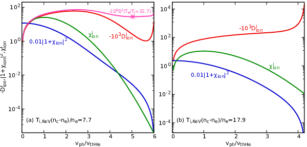
of $\omega_{\rm l}/\omega_{\rm pe}$ versus $k_{\rm l}\lambda_{\rm De}$ for EPW is calculated at different $m$ as shown in Fig. 3. For a given $k_{\rm l}\lambda_{\rm De}$, there are roughly three regimes in Fig. 3(a). In regime I, where $k_{\rm l}\lambda_{\rm De}\lesssim 0.43$, $\omega_{\rm l}$ decreases monotonously with $m$, and the dependence of the dispersion relation on $m$ is rather weak at about $k_{\rm l}\lambda_{\rm De}<0.2$. In regime II, where $0.43<k_{\rm l}\lambda_{\rm De}\lesssim 0.55$, the variation trend of $\omega_{\rm l}$ with $m$ becomes non-monotonous. In regime III, where $k_{\rm l}\lambda_{\rm De}>0.55$, $\omega_{\rm l}$ increases monotonously with $m$. In fact, for a fixed $k_{\rm l}\lambda_{\rm De}$, $\Delta\omega_{\rm l}/\Delta m=-(\partial\mathcal{Z}_{\rm e}/\partial m)/(\partial\mathcal{Z}_{\rm e}/\partial\omega_{\rm l})$ can be obtained from Eq. (12). It can be proven $\partial\mathcal{Z}_{\rm e}/\partial\omega_{\rm l}>0$ at the EPW frequency, but the sign of $\partial\mathcal{Z}_{\rm e}/\partial m$ depends on the value of $k_{\rm l}\lambda_{\rm De}$ and $m$, which results in the three regimes of different $k_{\rm l}\lambda_{\rm De}$. For the case I and case II shown in Fig. 2, by solving the dispersion relations Eq. (6) and Eq. (12) together with the matching conditions Eq. (5), $k_{\rm l}\lambda_{\rm De}$ can be obtained to be about $0.36$ for case I and $0.68$ for case II as indicated in Fig. 3(a). As expected, case I and case II are located in the regimes where $\lambda_{\rm R}$ is blue-shifted and red-shifted with $m$, respectively.

To understand the reason for the behavior of the peak value of $\mathrm{K}_{\rm R}$ with $m$ and the anti-correlation between the peak value and the half width of ${\mathrm{K}}_{\rm R}$,

can be deduced from Eq. (4), where the superscripts $\rm R$ and $\rm I$ denote the real and imaginary parts, respectively. According to Eq. (13), the half width is determined by $|1+\chi_{\rm e}^{\rm R}|\approx\chi_{\rm e}^{\rm I}$, so a higher peak value of ${\rm K}_{\rm R}$ is always related to a smaller half width of it. At the peak, $\chi_{\rm e}^{\rm R}+1\approx 0$, and the peak value of ${\mathrm{K}}_{\rm R}$ is proportional to $1/\chi_{\rm e}^{\rm I}$. Since $\chi_{\rm e}^{\rm I}=\nu_{\rm l}(\partial\epsilon^{\rm R}/\partial\omega)\approx\nu_{\rm l}(\partial\chi_{\rm e}^{\rm R}/\partial\omega)$ Strozzi2008RayBackScatter, it is $\nu_{\rm l}$ that primarily determines the trend of the peak value of ${\mathrm{K}}_{\rm R}$ with $m$. As shown in Fig. 3(b), $\nu_{\rm l}$ decreases with $m$ for all $k_{\rm l}\lambda_{\rm De}$, so the peak value of ${\mathrm{K}}_{\rm R}$ always increase with $m$. The trend of Landau damping with $m$ and $k_{\rm l}\lambda_{\rm De}$ can be understood from the feature of the EEDF near the matched phase velocity $v_{\rm ph}=\omega_{\rm l}/k_{\rm l}$. For $\nu_{\rm l}\ll\omega_{\rm l}$, $\chi_{\rm e}^{\rm I}$ from Eq. (8) can be written as

where second equality follows by using $\mathrm{Im}[1/(\omega/k-v_{x})]=-\pi\delta(\omega/k-v_{x})$ Chen1984Plasma. As shown in Fig. 4, in case I of small $k_{\rm l}\lambda_{\rm De}$, the matched $v_{\rm ph}$ is located in the tail of the EEDF where $\chi_{\rm e}^{\rm I}\propto e^{-v_{\rm ph}^{m}}$, and $\nu_{\rm l}$ decreases with $m$ rapidly. While in case II of large $k_{\rm l}\lambda_{\rm De}$, the matched $v_{\rm ph}$ is in the bulk region of the EEDF where $\chi_{\rm e}^{\rm I}(v_{\rm ph})$ at different $m$ is close. For such a case, it is the increase of the matched phase velocity with $m$ (see Fig. 3a) that leads to the decrease of Landau damping with $m$.

Commonly, SBS can occur in both the gas region with low-Z or mid-Z plasma and the ablated region with high-Z plasma in hohlraum Lindl2004ICFIndirectIgn. To illuminate the influence of super-Gaussian exponent $m$ on SBS, several examples with the typical parameters in hohlraum are shown in Figs. 5 and 6 for the low-Z and high-Z plasma with the specific conditions listed in Tables 1 and 2, respectively. In low-Z He and HHe plasma, we take $m=2,2.3,2.6,2.9$ as examples, while in high-Z Au and AuB plasma, $m=2,3,4,4.5$ are discussed. The intensity requirements for the corresponding $m$ of super-Gaussian EEDF, are listed in Tables 1 and  2 for these cases, which are possible due to the high intensity speckles and beam overlapping effects. Comparing different cases shown in Figs. 5 and 6, it is found that the peak wavelength of SBS backscattered light always increases with $m$ for a given parameter conditions and ion composition, but the influence of $m$ on the peak value of ${\rm K}_{\rm B}$ is much more complicated. In both He and HHe plasmas, the peak value of ${\rm K}_{\rm B}$ can increase or decrease with $m$ according to the plasma conditions. Even at the same condition labeled as case ‘a’, the variation trend of ${\rm K}_{\rm B}$ with $m$ can be opposite in He and HHe plasma. In high-Z case ‘d’, the peak $\mathrm{K}_{\rm B}$ decreases with $m$ in pure Au plasma, while the trend of the peak $\mathrm{K}_{\rm B}$ with $m$ becomes non-monotonic in AuB plasma, and depends sensitively on the isotopic type of the low-Z species $\rm B$.

To comprehend the behavior of ${\rm K}_{\rm B}$ with $m$, Eq. (4) can be written as

where

and superscripts $\mathrm{R}$ and $\mathrm{I}$ denote the real and imaginary parts, respectively. Near the peak of ${\rm K}_{\rm B}$, $\mathscr{D}^{\rm R}\approx 0$ is consistent with the dispersion relation of IAW $\epsilon\approx 0$ for weak damping $|\chi_{\rm e}^{\rm I}|\ll|\chi_{\rm e}^{\rm R}|$ and $|\chi_{\rm ion}^{\rm I}|\ll|1+\chi_{\rm ion}^{\rm R}|$, implying $\mathrm{K}_{\rm B}$ peaks near the natural resonance mode. And the peak value of spatial growth rate

To see the reason for the redshift of SBS backscattered light with $m$, the dispersion relation of IAW is solved. Under the approximation $\omega_{a}/k_{a}\ll v_{\rm the}$, for the super-Gaussian EEDF

Because $A_{m}$ increases with $m$ monotonically, $\chi_{\rm e}^{\rm R}$ decreases with $m$, implying a reduced number of slow electrons to shield the ions due to the Langdon effect Afeyan1998KinNonuniformHeating. For such $\chi_{\rm e}^{\rm R}$, the ion acoustic velocity $c_{\rm s}=\omega_{a}/k_{a}$ in plasma composed of one or two species Williams1995IAWTwoIon; Feng2020Laser3wto2w, is given by

where “$+$” corresponds to the fast mode, and “$-$” corresponds to the slow mode, and

and

Here $q\equiv 1+A_{m}k_{a}^{2}\lambda_{\rm De}^{2}$, $M_{\rm p}$ is the proton mass, the ion species is indicated by the subscript $\alpha=1,2$, $\gamma_{\alpha}$ is the adiabatic exponent, $A_{\alpha}$ is the mass number, and $f_{\alpha}$ is the number fraction of ion species $\alpha$. The bars denote the average, i.e.,

In the expression of $c_{\rm s}$, the term $A_{m}T_{\rm e}$ appears as a whole, so it can be thought that the Debye shielding electron temperature is effectively boosted to $A_{m}T_{\rm e}$. In Appendix A, it is proven that $c_{\rm s}$ increases with $A_{m}T_{\rm e}$ for both the fast and slow modes, when all other parameters such as $T_{\rm i}$ and $n_{\rm e}$ are kept constant. So it can be expected that due to the effective increase of Debye shielding electron temperature caused by a super-Gaussian EEDF, the IAW frequency $\omega_{a}=k_{a}c_{\rm s}$ increases with $m$. Consequently, the scattered wavelength $\lambda_{\rm B}=\omega_{0}\lambda_{0}/(\omega_{0}-\omega_{a})$ increases as $m$ increases.

From Eq. (17), the behavior of the peak value of ${\rm K}_{\rm B}$ with $m$ is primarily determined by the value of $-\mathscr{D}^{\rm I}$ near the peak wavelength. Since at the peak $\epsilon\approx 0$ and $|\chi_{\rm e}|\approx|1+\chi_{\rm ion}|$, it is found ${\rm K}_{\rm B}\propto-1/\mathscr{D}^{\rm I}\approx|\chi_{\rm e}||1+\chi_{\rm ion}|/(\chi_{\rm e}^{\rm I}+\chi_{\rm ion}^{\rm I})$. Considering that $\chi_{\rm e}^{\rm I}+\chi_{\rm ion}^{\rm I}=\mathrm{Im}[\epsilon]=(\nu_{\rm e}+\nu_{\rm ion})\partial\epsilon/\partial\omega$, where $\nu_{\rm e}$ and $\nu_{\rm ion}$ are electron and ion Landau damping rates respectively, and $|\chi_{\rm e}||1+\chi_{\rm ion}|$ is proportional to the ponderomotive drive for IAW Strozzi2008RayBackScatter, it can be understood that ${\rm K}_{\rm B}$ is determined by the tradeoff between the ponderomotive drive and the Landau damping of IAW. We can also separate out the ion and electron contributions to $\mathscr{D}^{\rm I}$,

with

and

At the peak of ${\rm K}_{\rm B}$, $\mathscr{D}_{\rm ion}^{\rm I}/\mathscr{D}_{\rm e}^{\rm I}\approx\chi_{\rm ion}^{\rm I}/\chi_{\rm e}^{\rm I}\approx\nu_{\rm ion}/\nu_{\rm e}$, so the relative contribution of electron and ion to $\mathscr{D}^{\rm I}$ is determined by the relative importance of electron Landau damping versus ion Landau damping. As shown in Fig. 4, the electron Landau damping reaches maximum when the phase velocity $v_{\rm ph}$ is close to $v_{\rm the}$. Similarly, the ion damping is maximum when the phase velocity $v_{\rm ph}$ is close to the ion thermal velocity $v_{\rm th\alpha}$. For SBS, typically $c_{\rm s}\ll v_{\rm the}$. When $Z_{\alpha}$ increase, the ion acoustic velocity $c_{\rm s}$ also increases, making the electron damping $\nu_{\rm e}$ increase whereas the ion damping $\nu_{\rm ion}$ decrease when $v_{\rm th\alpha}<c_{\rm s}$. The contribution of electron damping or ion damping can be quite different in low-Z and high-Z plasma. Furthermore, the possible super-Gaussian exponent $m$ due to Langdon effect is smaller in low-Z plasma than in high-Z plasma. Considering the differences in low-Z plasma and high-Z plasma, in the following, we discuss them separately.

In low-Z He and HHe plasmas, taking case ‘a’ as example, we show $-\mathscr{D}^{\rm I}$ in Fig. 7(a) and Fig. 8(a) for He and HHe plasmas, respectively. In proximity to the peak wavelength, $-\mathscr{D}^{\rm I}$ is mainly contributed by ions, because the ion damping which is proportional to $\chi_{\rm ion}^{\rm I}$ is much higher than the electron damping as shown in Figs. 7(b) and 8(b). Since the Maxwellian distribution of ions is assumed, $\mathscr{D}_{\rm ion}^{\rm I}$ itself does not depend on $m$. However, since the phase velocity of IAW corresponding to the peak wavelength $\lambda_{\rm B}$ increases with $m$, the decrease of $-\mathscr{D}^{\rm I}_{\rm ion}$ with the peak wavelength $\lambda_{\rm B}$ at different $m$ in He plasma leads to the increase of the peak value of $\mathrm{K}_{\rm B}$ with $m$. Similarly in HHe plasma, the increase of $-\mathscr{D}^{\rm I}_{\rm ion}$ with the peak wavelength $\lambda_{\rm B}$ at different $m$ results in the decrease of the peak $\mathrm{K}_{\rm B}$ with $m$.

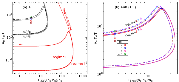
It can be concluded that the variation trend of peak $\mathrm{K}_{\rm B}$ with $m$ is determined by the behavior of $-\mathscr{D}^{\rm I}$ with $v_{\rm ph}$ near the phase velocity of IAW corresponding to the peak wavelength. According to this, two parameter regimes can be defined. In regime I, ${\partial\mathscr{D}^{\rm I}}/{\partial v_{\rm ph}}<0$ near the peak point and thus the peak $\mathrm{K}_{\rm B}$ decrease with $m$, while ${\partial\mathscr{D}^{\rm I}}/{\partial v_{\rm ph}}>0$ near the peak point and the peak $\mathrm{K}_{\rm B}$ increase with $m$ in regime II. So, the boundary between regime I and II satisfies ${\partial\mathscr{D}^{\rm I}}/{\partial v_{\rm ph}}=0$ at the peak point which maintains $\mathscr{D}^{\rm R}=0$. ¹¹ 1 In fact, it can be proven under the condition ${\partial\mathscr{D}^{\rm I}}/{\partial v_{\rm ph}}=0$ and $\mathscr{D}^{\rm R}=0$, $\mathrm{K}_{\rm B}$ given in Eq. (15) satisfies $\partial\mathrm{K}_{\rm B}/\partial\omega_{s}=0$. That is, the peak condition of $\mathrm{K}_{\rm B}$ is exactly satisfied. So when the weak dependence of $-\mathscr{D}_{\rm e}^{\rm I}$ on $m$ can be neglected, these two conditions give the exact conditions for the boundary where the trend of the peak $\mathrm{K}_{\rm B}$ with $m$ changes. These two equations determine a relation between $A_{m}T_{\rm e}/T_{\rm i}$ and $T_{\rm i}(1-n_{\rm e}/n_{\rm c})/n_{\rm e}$ for a given ion composition. By numerical solution, the boundary between regime I and II for He and HHe plasma are shown in Fig. 9, where the weak dependence of $-\mathscr{D}_{\rm e}^{\rm I}$ on $m$ is ignored, and the different cases shown in Fig. 5 are also labelled as asterisks. As expected, case ‘b’ is located in regime I of He plasma, and case ‘c’ is located in regime II of HHe plasma. Case ‘a’ of He and HHe are located in the special parameter range that is in regime II of He plasma yet in regime I of HHe plasma, thus the variation trend of peak $\mathrm{K}_{\rm B}$ with $m$ are opposite in case ‘a’ of He and HHe plasma even under the same parameter condition.

Now we take a closer look into the case ‘a’ to comprehend the physical mechanism for the effects of mixture. Since $-\mathscr{D}_{\rm ion}^{\rm I}=\chi_{\rm ion}^{\rm I}/|1+\chi_{\rm ion}|^{2}$ dominates $-\mathscr{D^{\rm I}}$ near the matched $c_{\rm s}$ as discussed above, and both $\chi_{\rm ion}^{\rm I}$ and $|1+\chi_{\rm ion}|^{2}$ drop with $v_{\rm ph}$, the relative dropping rate of $\chi_{\rm ion}^{\rm I}$ and $|1+\chi_{\rm ion}|^{2}$ with $v_{\rm ph}$ determines the sign of ${\partial\mathscr{D}^{\rm I}}/{\partial v_{\rm ph}}$ and thus the regime. In Fig. 10, the dropping rate of $\chi_{\rm ion}^{\rm I}$ and $|1+\chi_{\rm ion}|^{2}$, which are defined as $\partial(\ln\chi_{\rm ion}^{\rm I})/\partial v_{\rm ph}$ and $\partial(\ln|1+\chi_{\rm ion}|^{2})/\partial v_{\rm ph}$ respectively, are shown as the function of $v_{\rm ph}$ for H, He and HHe (1:1) with the same plasma parameters in case ‘a’, as well as the matched phase velocity corresponding to the peak ${\rm K}_{\rm B}$ at different $m$ for each ion composition. The $v_{\rm ph}$ and the dropping rate are normalized by thermal velocity of helium $v_{\rm thHe}$ and $1/v_{\rm thHe}$, respectively. As expected, in HHe plasma, the matched $c_{\rm s,HHe}$ is between the matched $c_{\rm s,H}$ in single-species H plasma and $c_{\rm s,He}$ in single-species He plasma, with $c_{\rm s,HHe}/v_{\rm thHe}\sim 4$ and $c_{\rm s,HHe}/v_{\rm thH}\sim 2$. Because $c_{\rm s,HHe}$ is closer to $v_{\rm thH}$, the Landau damping is mainly contributed by H ions, and the dropping rate of $\chi_{\rm HHe}^{\rm I}$ is closer to $\chi_{\rm H}^{\rm I}$ in case of single H ions, as shown in Fig. 10. However, due to the contributions of He ions, the dropping rate of $|1+\chi_{\rm HHe}|^{2}$ is larger than $|1+\chi_{\rm H}|^{2}$ of the single H case. As a consequence, the decrease of $\chi_{\rm HHe}^{\rm I}$ with $v_{\rm ph}$ is slower than the decrease of $|1+\chi_{\rm HHe}|^{2}$ in HHe plasma near $c_{\rm s,HHe}$, which leads to ${\partial\mathscr{D}^{\rm I}}/{\partial v_{\rm ph}}<0$ and thus in regime I in case ‘a’.

In Fig. 9, the regime II is constrained between a limited range of $A_{\rm m}T_{\rm e}/T_{\rm i}$ when $T_{\rm i}(1-n_{\rm e}/n_{\rm c})/n_{\rm e}$ is small, while it is totally regime I when $T_{\rm i}(1-n_{\rm e}/n_{\rm c})/n_{\rm e}$ is large enough. This general feature of the partition between regime I and II can be explained as follows. When $T_{\rm i}(1-n_{\rm e}/n_{\rm c})/n_{\rm e}$ is large enough, $-\mathscr{D}^{\rm I}_{\rm ion}$ increases with $v_{\rm ph}$ for all possible $v_{\rm ph}$ of IAW, as shown in Fig. 11(b). Since $-\mathscr{D}^{\rm I}_{\rm e}$ also increases (linearly) with $v_{\rm ph}$ for $v_{\rm ph}\ll v_{\rm the}$, $-\mathscr{D}^{\rm I}$ increases with $v_{\rm ph}$ over the entire range of all possible $c_{\rm s}$, rendering such $T_{\rm i}(1-n_{\rm e}/n_{\rm c})/n_{\rm e}$ belonging to regime I for all $A_{m}T_{\rm e}/T_{\rm i}$. When $T_{\rm i}(1-n_{\rm e}/n_{\rm c})/n_{\rm e}$ is smaller, as $v_{\rm ph}$ increases, $-\mathscr{D}^{\rm I}_{\rm ion}$ increases to a maximum firstly then decreases to a minimum, because $\chi_{\rm ion}^{\rm I}$ drops with $v_{\rm ph}$ faster and faster after $v_{\rm ph}>v_{\rm th\alpha}$, and its dropping rate exceeds the dropping rate of $|1+\chi_{\rm ion}|^{2}$ beyond this maximum point, as shown in Fig. 11(a). While the minimum point arises because $-\mathscr{D}^{\rm I}_{\rm ion}$ rises sharply towards a peak at large $v_{\rm ph}$ where $\chi_{\rm ion}+1$ approaches zero. This peak corresponds to the greatest possible matched $c_{\rm s}$ when $A_{m}T_{\rm e}\gg T_{\rm i}$, and $\chi_{\rm e}\ll 1$ is negligible in the dispersion equation $\epsilon\approx 1+\chi_{\rm ion}=0$. For a given $T_{\rm i}$, the matched $c_{\rm s}$ increases with the increased $A_{\rm m}T_{\rm e}/T_{\rm i}$, consequently, the ion damping decreases while the electron damping increases, as shown in Figs. 7(b) and 8(b). When $A_{\rm m}T_{\rm e}/T_{\rm i}$ is small enough, the contribution of $-\mathscr{D}^{\rm I}_{\rm ion}$ dominates. The boundary coincides with the boundary when only the ion damping considered alone as shown in Fig. 9. The lower boundary corresponds to the maximum point of $-\mathscr{D}^{\rm I}_{\rm ion}$. For a parameter point with $A_{\rm m}T_{\rm e}/T_{\rm i}$ located below the lower boundary, the matched $c_{\rm s}$ is on the left side of the phase velocity corresponding to the maximum point of $-\mathscr{D}_{\rm ion}^{\rm I}$, thus $-\mathscr{D}^{\rm I}$ increases with $v_{\rm ph}$ and this parameter point is in regime I. While for a parameter point with $A_{\rm m}T_{\rm e}/T_{\rm i}$ located above the lower boundary, the matched $c_{\rm s}$ is on the right side of the maximum point, thus $-\mathscr{D}^{\rm I}$ decreases with $v_{\rm ph}$ and this parameter point is in regime II. With the increase of $A_{\rm m}T_{\rm e}/T_{\rm i}$, the matched $c_{\rm s}$ becomes closer and closer to the minimum point of $-\mathscr{D}_{\rm ion}^{\rm I}$, but $-\mathscr{D}_{\rm e}^{\rm I}$ which increases with $v_{\rm ph}$ becomes more and more important. At the upper right boundary of regime II with a relatively large $T_{\rm i}(1-n_{\rm e}/n_{\rm c})/n_{\rm e}$, $c_{\rm s}$ reaches the minimum point before $-\mathscr{D}_{\rm e}^{\rm I}$ becomes sufficiently important. While for smaller $T_{\rm i}(1-n_{\rm e}/n_{\rm c})/n_{\rm e}$, the increase of $-\mathscr{D}_{\rm e}^{\rm I}$ with $v_{\rm ph}$ completely cancels the decrease of $-\mathscr{D}_{\rm ion}^{\rm I}$ with $v_{\rm ph}$ before the phase velocity approaches the minimum point of $-\mathscr{D}_{\rm ion}^{\rm I}$ as shown in Fig. 11(a), where the asterisk symbol indicates the location of the phase velocity corresponding to the minimum point of $-\mathscr{D}^{\rm I}$ with consideration of electron damping. This minimum point of $-\mathscr{D}^{\rm I}$ corresponds to the upper boundary of regime II at small $T_{\rm i}(1-n_{\rm e}/n_{\rm c})/n_{\rm e}$ in Fig. 9.

In high-Z plasmas, the Langdon effect can be more significant and the super-Gaussian exponent can approach about $5$. With the same definition of parameter regimes discussed above, the boundary between regime I and II is shown in Fig. 12 for Au and AuB plasma (including both Au¹⁰B and Au¹¹B), respectively. Since the weak dependence of $-\mathscr{D}_{\rm e}^{\rm I}$ on $m$, the parameter boundary shifts with $m$ indistinctly as shown in Fig. 12(b). Here, only the boundary at $m=2$ is shown for Au plasma. It is noticed that when the ion damping is considered alone, the regime II of AuB plasma is enclosed in the regime II of Au plasma. In fact, this holds generally for mixing low-Z species into the single ion species plasma with higher charge state. However, taking into account contributions from the electron damping, parameter region of regime II of Au plasma is reduced, and the regime II of AuB plasma locates inside the regime I of Au plasma. An interesting point of Fig. 12 is that the boundary of regime II for Au¹⁰B plasma is upwardly shifted relative to that for Au¹¹B plasma. Such an isotope effect should be embodied especially near the boundary of regime II. As shown in Fig. 12 case ‘d’ belongs to regime I in Au plasma, and spans both regime I and II in AuB plasma. Thus, as expected, the peak $\mathrm{K}_{\rm B}$ decreases with $m$ monotonically in Au plasma, while the trend of the peak $\mathrm{K}_{\rm B}$ with $m$ becomes non-monotonic and depends sensitively on the isotopic type of the low-Z species $\rm B$ in AuB plasma, as shown in Fig. 6.

Using case ‘d’ as example, we take a closer look into the effects of the super-Gaussian EEDF and mixture near the upper boundary between regime I and II. In Au plasma, the electron damping dominates over the negligible ion damping since the matched $c_{\rm s}$ corresponding to the peak ${\rm K}_{\rm B}$ is much larger than ion thermal velocity $v_{\rm thAu}$, $-\mathscr{D}^{\rm I}\approx-\mathscr{D}_{\rm e}^{\rm I}$ increases with the matched phase velocity $c_{\rm s}$ and hence $\lambda_{\rm B}$, but decreases with $m$ as shown in Fig. 13(b). The first effect has a greater impact in case ‘d’, which leads the peak ${\rm K}_{\rm B}$ decrease with $m$ as shown in Fig. 13(a). After mixing the low-Z boron species into Au plasma, the variation of the ion damping with $v_{\rm ph}$ due to B ions is not negligible compared to the variation of electron damping with $v_{\rm ph}$, as shown in Fig. 14(b). Furthermore, $-\mathscr{D}_{\rm ion}^{\rm I}$ decreases with $\lambda_{\rm B}$ whereas $-\mathscr{D}_{\rm e}^{\rm I}$ increases with $\lambda_{\rm B}$. The trend of the peak $\mathrm{K}_{\rm B}$ with $m$ depends on the competition of the opposite change of $-\mathscr{D}_{\rm e}^{\rm I}$ and $-\mathscr{D}_{\rm ion}^{\rm I}$ with $\lambda_{\rm B}$. In Au¹¹B plasma, this competition effect is the main reason for the non-monotonic change of the peak ${\rm K}_{\rm B}$ with $m$. Nevertheless, the obviously high $-\mathscr{D}^{\rm I}$ at $m=2$ as shown in Fig. 14(a) leads the significant lower value of peak ${\rm K}_{\rm B}$ at $m=2$ than $m=3,4,5$ as shown in Fig. 6(b). Compared to ¹¹B ion, the lighter ¹⁰B ion has a larger thermal velocity as shown in Fig. 14(b). As a result, near the peak wavelength, the ion damping contributed by ¹⁰B is larger than ¹¹B. On one hand, this leads to a smaller ${\rm K}_{\rm B}$ in Au¹⁰B than in Au¹¹B plasma as shown in Fig. 6(b). On the other hand, it makes the contribution of $-\mathscr{D}_{\rm ion}^{\rm I}$ to $-\mathscr{D}^{\rm I}$ become larger in Au¹⁰B plasma, which leads to a stronger decreasing trend of $-\mathscr{D}^{\rm I}$ with $\lambda_{\rm B}$ as shown in Fig. 14(a). Thus, the peak ${\rm K}_{\rm B}$ increase with $m$ in Au¹⁰B plasma as shown in Fig. 6(b).

References

- (1) A. Bruce Langdon. Nonlinear inverse bremsstrahlung and heated-electron distributions. Physical Review Letters, 44(9):575–579, 1980.
- (2) J P Matte, M Lamoureux, C Moller, R Y Yin, J Delettrez, J Virmont, and T W Johnston. Non-Maxwellian electron distributions and continuum X-ray emission in inverse Bremsstrahlung heated plasmas. Plasma Physics and Controlled Fusion, 30(12):1665–1689, 1988.
- (3) Su Ming Weng, Zheng Ming Sheng, and Jie Zhang. Inverse bremsstrahlung absorption with nonlinear effects of high laser intensity and non-Maxwellian distribution. Physical Review E - Statistical, Nonlinear, and Soft Matter Physics, 80(5):1–5, 2009.
- (4) David Turnbull, Arnaud Colaïtis, Aaron M. Hansen, Avram L. Milder, John P. Palastro, Joseph Katz, Christophe Dorrer, Brian E. Kruschwitz, David J. Strozzi, and Dustin H. Froula. Impact of the Langdon effect on crossed-beam energy transfer. Nature Physics, 16:181–185, 2020.
- (5) Jian Zheng, C. X. Yu, and Z. J. Zheng. Effects of non-maxwellian (super-gaussian) electron velocity distribution on the spectrum of thomson scattering. Physics of Plasmas, 4(7):2736–2740, 1997.
- (6) A. L. Milder, H. P. Le, M. Sherlock, P. Franke, J. Katz, S. T. Ivancic, J. L. Shaw, J. P. Palastro, A. M. Hansen, I. A. Begishev, W. Rozmus, and D. H. Froula. Evolution of the electron distribution function in the presence of inverse bremsstrahlung heating and collisional ionization. Phys. Rev. Lett., 124:025001, 2020.
- (7) John D. Lindl, Peter Amendt, Richard L. Berger, S. Gail Glendinning, Siegfried H. Glenzer, Steven W. Haan, Robert L. Kauffman, Otto L. Landen, and Laurence J. Suter. The physics basis for ignition using indirect-drive targets on the national ignition facility. Physics of Plasmas, 11(2):339–491, 2004.
- (8) Liang Hao, Yiqing Zhao, Dong Yang, Zhanjun Liu, Xiaoyan Hu, Chunyang Zheng, Shiyang Zou, Feng Wang, Xiaoshi Peng, Zhichao Li, Sanwei Li, Tao Xu, and Huiyue Wei. Analysis of stimulated raman backscatter and stimulated brillouin backscatter in experiments performed on sg-iii prototype facility with a spectral analysis code. Physics of Plasmas, 21(7):072705, 2014.
- (9) D. J. Strozzi, E. A. Williams, D. E. Hinkel, D. H. Froula, R. A. London, and D. A. Callahan. Ray-based calculations of backscatter in laser fusion targets. Physics of Plasmas, 15(10):102703, 2008.
- (10) G. N. Hall, O. S. Jones, D. J. Strozzi, J. D. Moody, D. Turnbull, J. Ralph, P. A. Michel, M. Hohenberger, A. S. Moore, O. L. Landen, L. Divol, D. K. Bradley, D. E. Hinkel, A. J. Mackinnon, R. P. J. Town, N. B. Meezan, L. Berzak Hopkins, and N. Izumi. The relationship between gas fill density and hohlraum drive performance at the national ignition facility. Physics of Plasmas, 24(5):052706, 2017.
- (11) D. J. Strozzi, D. S. Bailey, P. Michel, L. Divol, S. M. Sepke, G. D. Kerbel, C. A. Thomas, J. E. Ralph, J. D. Moody, and M. B. Schneider. Interplay of laser-plasma interactions and inertial fusion hydrodynamics. Phys. Rev. Lett., 118:025002, 2017.
- (12) V Yu Bychenkov, W Rozmus, and V T Tikhonchuk. Stimulated Raman scattering in non-Maxwellian plasmas. Physics of Plasmas, 4(5):1481, 1997.
- (13) Bedros B. Afeyan, Albert E. Chou, J. P. Matte, R. P. J. Town, and William J. Kruer. Kinetic theory of electron-plasma and ion-acoustic waves in nonuniformly heated laser plasmas. Phys. Rev. Lett., 80:2322–2325, 1998.
- (14) P. Neumayer, R. L. Berger, L. Divol, D. H. Froula, R. A. London, B. J. MacGowan, N. B. Meezan, J. S. Ross, C. Sorce, L. J. Suter, and S. H. Glenzer. Suppression of stimulated brillouin scattering by increased landau damping in multiple-ion-species hohlraum plasmas. Phys. Rev. Lett., 100:105001, 2008.
- (15) P. Neumayer, R. L. Berger, D. Callahan, L. Divol, D. H. Froula, R. A. London, B. J. MacGowan, N. B. Meezan, P. A. Michel, J. S. Ross, C. Sorce, K. Widmann, L. J. Suter, and S. H. Glenzer. Energetics of multiple-ion species hohlraum plasmas. Physics of Plasmas, 15(5):056307, 2008.
- (16) J. F. Drake, P. K. Kaw, Y. C. Lee, G. Schmid, C. S. Liu, and Marshall N. Rosenbluth. Parametric instabilities of electromagnetic waves in plasmas. The Physics of Fluids, 17(4):778–785, 1974.
- (17) Francis F Chen. Introduction to plasma physics and controlled fusion, volume 1. Springer, 1984.
- (18) R. K. Kirkwood, J. D. Moody, J. Kline, E. Dewald, S. Glenzer, L. Divol, P. Michel, D. Hinkel, R. Berger, E. Williams, J. Milovich, L. Yin, H. Rose, B. Macgowan, O. Landen, M. Rosen, and J. Lindl. A review of laser-plasma interaction physics of indirect-drive fusion. Plasma Physics and Controlled Fusion, 55(10):103001, 2013.
- (19) E. A. Williams, R. L. Berger, R. P. Drake, A. M. Rubenchik, B. S. Bauer, D. D. Meyerhofer, A. C. Gaeris, and T. W. Johnston. The frequency and damping of ion acoustic waves in hydrocarbon (ch) and two-ion-species plasmas. Physics of Plasmas, 2(1):129–138, 1995.
- (20) Q.S. Feng, Z.J. Liu, L.H. Cao, C.Z. Xiao, L. Hao, C.Y. Zheng, C. Ning, and X.T. He. Interaction of parametric instabilities from 3 and 2 lasers in large-scale inhomogeneous plasmas. Nuclear Fusion, 60(6):066012, 2020.
Appendix A Proof that the ion acoustic velocity is monotonically increasing with
The ion acoustic velocity is given by Eq. (19) as , with the plus for the fast mode, and the minus for the slow mode. Firstly we define