跳到论文正文
W Papers独立论文阅读器 arXiv:2011.07434 论文正文 计算阅读时间 · 0%
引用这篇论文根据当前论文元数据生成,正式投稿前建议核对。


License: CC BY 4.0
arXiv:2011.07434v2 [math.NA] 31 Mar 2022

Time-Domain Multiple Traces Boundary Integral Formulation for Acoustic Wave Scattering in 2D

Carlos Jerez-Hanckes Thanks: (carlos.jerez@uai.cl), Faculty of Engineering and Sciences, Universidad Adolfo Ibáñez, Santiago, Chile    Ignacio Labarca Thanks: (ignacio.labarca@sam.math.ethz.ch), Seminar for Applied Mathematics, Swiss Federal Institute of Technology, Zurich, Switzerland
Abstract

We present a novel computational scheme to solve acoustic wave transmission problems over two-dimensional composite scatterers, i.e. penetrable obstacles possessing junctions or triple points. The continuous problem is cast as a multiple traces time-domain boundary integral formulation. For discretization in time and space, we resort to convolution quadrature schemes coupled to a non-conforming spatial spectral discretization based on second kind Chebyshev polynomials displaying fast convergence. Computational experiments confirm convergence of multistep and multistage convolution quadrature for a variety of complex domains.

Keywords: acoustic wave scattering, wave transmission problems, convolution quadrature, time-domain boundary integral operators, multiple traces formulation

1 Introduction

We are interested in solving acoustic wave transmission problems arising from the scattering by composite objects in two dimensions. More precisely, we consider a bounded Lipschitz domain Ω⊂ℝ2\Omega\subset\mathbb{R}^{2}, composed of MM non-overlapping Lipschitz subdomains Ωi\Omega_{i}, i=1,…,M,i=1,\ldots,M, such that

Ω¯=⋃i=1MΩ¯i,\overline{\Omega}=\bigcup_{i=1}^{M}\overline{\Omega}_{i}, (1)

where Ωi∩Ωj=∅\Omega_{i}\cap\Omega_{j}=\emptyset for i≠ji\neq j. We define Γi​j:=∂Ωi∩∂Ωj\Gamma_{ij}:=\partial\Omega_{i}\cap\partial\Omega_{j} for the interface between domains Ωi\Omega_{i} and Ωj\Omega_{j}, with Γi​j=Γj​i\Gamma_{ij}=\Gamma_{ji}. We also denote by Ω0:=ℝd\Ω¯\Omega_{0}:=\mathbb{R}^{d}\ \backslash\ \overline{\Omega} the unbounded exterior domain. Notice that, for i=0,…,M,i=0,\ldots,M, one can write

Γi:=∂Ωi=⋃j∈ΥiΓi​j,\Gamma_{i}:=\partial\Omega_{i}=\bigcup_{j\in\Upsilon_{i}}\Gamma_{ij},

where Υi\Upsilon_{i} corresponds to an index set defined as

Υi:={j∈{0,…,M}:j≠i and Γi​j≠∅}.\Upsilon_{i}:=\left\{j\in\{0,\ldots,M\}:\quad j\neq i\text{ and }\Gamma_{ij}\neq\emptyset\right\}.

The above composite material is characterized by piecewise-constant coefficients, ci>0c_{i}>0 corresponding to the wavespeed on the domain Ωi\Omega_{i}, i=0,…,Mi=0,\ldots,M. Assuming some incoming wave with no volume sources denoted uincu^{\text{inc}}, we set ui:=u|Ωiu_{i}:=u|_{\Omega_{i}} for the total wave inside Ωi\Omega_{i}, for i=1,…,Mi=1,\ldots,M, and by u0:=u|Ω0u_{0}:=u|_{\Omega_{0}} the scattered wave in the exterior domain. With this, we seek to solve the time-domain acoustic transmission problem:

{1ci2​∂2ui∂t2−Δ​ui=0 in ​Ωi×[0,∞),i=0,…,M,u0−uj=−uinc on ​Γ0​j×[0,∞),j∈Υ0,∂u0∂n0+∂uj∂nj=−∂uinc∂n0 on ​Γ0​j×[0,∞),j∈Υ0,ui−uj=0 on ​Γi​j×(0,∞],i,j>0,j∈Υi,∂ui∂ni+∂uj∂nj=0 on ​Γi​j×[0,∞),i,j>0,j∈Υi,ui=∂ui∂t=0 in ​Ωi×{0},i=0,…,M.\left\{\begin{array}[]{ll}\dfrac{1}{c_{i}^{2}}\dfrac{\partial^{2}u_{i}}{\partial t^{2}}-\Delta u_{i}=0&\text{ in }\Omega_{i}\times[0,\infty),\quad i=0,\ldots,M,\\ &\\ u_{0}-u_{j}=-u^{\text{inc}}&\text{ on }\Gamma_{0j}\times[0,\infty),\ j\in\Upsilon_{0},\\ &\\ \dfrac{\partial u_{0}}{\partial n^{0}}+\dfrac{\partial u_{j}}{\partial n^{j}}=-\dfrac{\partial u^{\text{inc}}}{\partial n^{0}}&\text{ on }\Gamma_{0j}\times[0,\infty),\ j\in\Upsilon_{0},\\ &\\ u_{i}-u_{j}=0&\text{ on }\Gamma_{ij}\times(0,\infty],\ i,j>0,\ j\in\Upsilon_{i},\\ &\\ \dfrac{\partial u_{i}}{\partial n^{i}}+\dfrac{\partial u_{j}}{\partial n^{j}}=0&\text{ on }\Gamma_{ij}\times[0,\infty),\ i,j>0,\ j\in\Upsilon_{i},\\ &\\ u_{i}=\dfrac{\partial u_{i}}{\partial t}=0&\text{ in }\Omega_{i}\times\{0\},i=0,\ldots,M.\end{array}\right. (2)
Figure 1: Example of a scatterer with two homogenous subdomains.

We solve the above wave scattering problem by combining the following approaches:

  1. (i)

    Boundary integral equations (BIEs) in the form of the local multiple traces formulation (MTF) in space-time domain;

  2. (ii)

    Spectral non-conforming Galerkin discretizations with Chebyshev polynomials for spatial discretization of the BIEs; and,

  3. (iii)

    Convolution quadrature (CQ) for approximation in time.

BIEs lead to unknowns defined on boundaries while rigorously enforcing causality or radiation conditions in the time-harmonic case [29]. Specifically, for composite materials one can resort to BIEs based on single-trace formulations or different versions of MTFs according to the strong or weak enforcement of transmission conditions (cf. [19, 6, 7]). The discretization of MTFs then may be carried out via boundary elements (BE) [19, 18], spectral Galerkin [22, 23, 17] or Nyström [21] methods.

In the following, we employ a spatial spectral non-conforming discrete Galerkin scheme for the (local) MTF based on Chebyshev polynomials in order to attain accurate approximations with a small number of degrees of freedom. Moreover, this setting allows for the efficient computation of matrix entries via the Fast Fourier Transform (FFT) by relating Chebyshev coefficients to Fourier coefficients as well as direct implementation of compression techniques (cf. [22, Section 3.3], [23] and [35, Chapter 3]). First and second kind single-trace formulations [8, 13] also exist but there are no available spectrally convergent methods for them. Still, due to the non-conforming nature of our spectral scheme, its numerical analysis remains open an open problem as existing results require Galerkin discretization in standard Sobolev spaces. Thus, the present work focuses on algorithmic aspects. Indeed, though we introduce the required functional spaces for rigorously formulating the MTF, these are not essential for neither the current presentation nor its implementation. For a precise derivation and results of existence and uniqueness of the continuous problem we refer to [19].

For the time-domain approximation we opt for CQ methods [5, 33] due to their stability and amenability to be coupled to any available complex frequency-domain solvers such as the ones discussed above. Algorithmically, we refer to [15] for the corresponding pseudo-code to efficiently compute forward convolutions and solve the arising equations. A thorough analysis of multistage CQ can be found in [1, 2, 3, 28], while generalized CQ allowing for different timesteps is described in [24, 25]. CQ implementation and analysis for wave scattering problems have been studied in [4], with emphasis on transmission problems provided in [30, 31] and composite materials in [32, 13]. Yet, to our knowledge, no time-domain CQ-MTF has been described in the literature, with the current work being the first contribution to that end.

Alternatively, direct Galerkin discretizations for space-time BIEs could also be used to tackle Problem (2), but this involves the difficult computation of boundary integral operators in time domain [5]. Moreover, as it happens in most time-stepping procedures, a poor choice of time-step may immediately lead to instabilities. Also, long-time computations are often unstable and despite the availability of several remedies (cf. [9, 10, 11, 12]), CQ remains a simple, efficient and stable method to discretize time-domain problems without major complications.

The present manuscript is structured as follows. In Section 2, we present the MTF in frequency domain as in [19]. Section 3 recalls the main ideas behind time-domain BIEs. Section 4 describes the spatial spectral non-conforming Galerkin discretization for MTF [22, 23]. Then, in Sections 5.1 and 5.2 we explain CQ for multistep and multistage linear methods and their application to convolutional equations in Section 5.3. Finally, in Section 6 we show some numerical experiments for different geometries and parameters of interest, which clearly illustrate the capabilities and limitations of the proposed methodology and sketch future research ideas.

Besides the definitions already introduced, the notation used throughout can be summarized as follows:

  • •

    The imaginary unit is denoted ı=−1\imath=\sqrt{-1}.

  • •

    uu denotes an acoustic field in space and time (see (2)).

  • •

    UU and VV denote Laplace-domain fields related to the modified Helmholtz equation (see Section 2).

  • •

    λ,φ,ψ\lambda,\varphi,\psi denote time-domain boundary densities, with values in Sobolev spaces defined over a boundary or interface (see Section 3, (16) and Problem 3.1).

  • •

    Λ,Φ,Ψ\Lambda,\Phi,\Psi are boundary functions in frequency domain (see Section 2, (11), (7)).

  • •

    Bold variables 𝝀,𝝋,𝒈,𝚲,𝚽,𝑮\bm{\lambda},\ \bm{\varphi},\ \bm{g},\ \bm{\Lambda},\ \bm{\Phi},\ \bm{G} denote elements of Cartesian product spaces (see Problems 2.2, 3.1, 4.3, 5.2 and 5.4).

  • •

    Operators 𝖠,𝖲,𝖣,𝖪,𝖪′,𝖵,𝖶,𝖷,𝖤,𝖱,𝖫\mathsf{A},\mathsf{S},\mathsf{D},\mathsf{K},\mathsf{K}^{\prime},\mathsf{V},\mathsf{W},\mathsf{X},\mathsf{E},\mathsf{R},\mathsf{L} are defined in the frequency domain, sometimes depending on a complex parameter s∈ℂ+s\in\mathbb{C}_{+} (see Section 2, (7), (9), (10)).

  • •

    Operators 𝒜,𝒮,𝒟,𝒦,𝒦′,𝒱,𝒲,ℱ\mathcal{A},\mathcal{S},\mathcal{D},\mathcal{K},\mathcal{K}^{\prime},\mathcal{V},\mathcal{W},\mathcal{F} are defined in the time domain by means of the inverse Laplace transform of frequency domain counterparts (see Section 3, (16), (17), (18) and Problem 3.1).

  • •

    NN is the number of timesteps (see Problem 5.2).

  • •

    LL refers to the number of degrees of freedom of the spectral spatial discretization (see Section 4.1, Problem (4.3)).

  • •

    Variable s∈ℂ+s\in\mathbb{C}_{+} is reserved for the parameter in Laplace domain and modified Helmholtz equations (see Section 2, (6), (7), (8), (9)).

2 Multiple traces formulation

We recall results for the (local) MTF for Helmholtz scattering problems over composite materials as exposed in [19, 23]. Despite being initially developed for time-harmonic problems, the formulation lends itself easily to account for time-dependent wave scattering via the inverse Laplace transform as discussed in Section 3.

Let Ω⊂ℝ2\Omega\subset\mathbb{R}^{2} be as in (1) and 𝒏i\bm{n}^{i} denote the unit outward normal vector to ∂Ωi\partial\Omega_{i}. Trace spaces on the boundary are written H±1/2(∂Ωi)H^{\pm 1/2}(\partial\Omega_{i}). For an open interface Γi​j\Gamma_{ij}, we introduce

H12​(Γi​j):={ξ|Γi​j:ξ∈H12​(∂Ωi)} and H~12​(Γi​j):={η∈H12​(Γi​j):η~∈H12​(∂Ωi)},H^{\frac{1}{2}}(\Gamma_{ij}):=\{\xi|_{\Gamma_{ij}}\ :\ \xi\in H^{\frac{1}{2}}(\partial\Omega_{i})\}\quad\text{ and }\quad\widetilde{H}^{\frac{1}{2}}(\Gamma_{ij}):=\{\eta\in H^{\frac{1}{2}}(\Gamma_{ij})\ :\ \widetilde{\eta}\in H^{\frac{1}{2}}(\partial\Omega_{i})\},

where η~\tilde{\eta} is the extension by zero of η\eta over ∂Ωi\partial\Omega_{i}. We identify H~−12​(Γi​j)\widetilde{H}^{-\frac{1}{2}}(\Gamma_{ij}) with the dual space of H12​(Γi​j)H^{\frac{1}{2}}(\Gamma_{ij}). Cartesian product trace spaces over closed boundaries ∂Ωi\partial\Omega_{i} are denoted

𝐕i:=H12​(∂Ωi)×H−12​(∂Ωi).\mathbf{V}_{i}:=H^{\frac{1}{2}}(\partial\Omega_{i})\times H^{-\frac{1}{2}}(\partial\Omega_{i}).

For the multiple interfaces case we require the following piecewise or broken spaces:

H~pw∓12(∂Ωi):={V∈H∓12(∂Ωi):V|Γi​j∈H~∓12(Γi​j),∀j∈Υi},\widetilde{H}_{\text{pw}}^{\mp\frac{1}{2}}(\partial\Omega_{i}):=\left\{V\in H^{\mp\frac{1}{2}}(\partial\Omega_{i})\ :\ V|_{\Gamma_{ij}}\in\widetilde{H}^{\mp\frac{1}{2}}(\Gamma_{ij}),\quad\forall j\in\Upsilon_{i}\right\}, (3)

whose respective duals are

Hpw±12(∂Ωi):={V∈𝒟′(∂Ωi):V|Γi​j∈H±12(Γi​j),∀j∈Υi},H_{\text{pw}}^{\pm\frac{1}{2}}(\partial\Omega_{i}):=\left\{V\in\mathcal{D}^{\prime}(\partial\Omega_{i})\ :\ V|_{\Gamma_{ij}}\in H^{\pm\frac{1}{2}}(\Gamma_{ij}),\quad\forall j\in\Upsilon_{i}\right\}, (4)

where 𝒟′​(∂Ωi)\mathcal{D}^{\prime}(\partial\Omega_{i}) denotes the space of distributions over ∂Ωi\partial\Omega_{i}. With (3) and (4) we define the broken Cartesian product spaces:

𝐕pw,i:=Hpw12​(∂Ωi)×Hpw−12​(∂Ωi) and 𝐕~~i:=H~pw12​(∂Ωi)×H~pw−12​(∂Ωi).\mathbf{V}_{\text{pw},i}:=H^{\frac{1}{2}}_{\text{pw}}(\partial\Omega_{i})\times H^{-\frac{1}{2}}_{\text{pw}}(\partial\Omega_{i})\quad\text{ and }\quad\widetilde{\raisebox{0.0pt}[0.85pt]{$\widetilde{\mathbf{V}}$}}_{i}:=\widetilde{H}^{\frac{1}{2}}_{\text{pw}}(\partial\Omega_{i})\times\widetilde{H}^{-\frac{1}{2}}_{\text{pw}}(\partial\Omega_{i}).

Furthermore, we build the next spaces defined over M∈ℕM\in\mathbb{N} subdomain boundaries:

𝕍~~M:⁣=𝐕~~0×…×𝐕~~M,𝕍M:⁣=𝐕0×…×𝐕M,𝕍pw,M:⁣=𝐕pw,0×…×𝐕pw,M.\begin{array}[]{rcl}\widetilde{\raisebox{0.0pt}[0.85pt]{$\widetilde{\mathbb{V}}$}}_{M}&:=&\widetilde{\raisebox{0.0pt}[0.85pt]{$\widetilde{\mathbf{V}}$}}_{0}\times\ldots\times\widetilde{\raisebox{0.0pt}[0.85pt]{$\widetilde{\mathbf{V}}$}}_{M},\\ \mathbb{V}_{M}&:=&\mathbf{V}_{0}\times\ldots\times\mathbf{V}_{M},\\ \mathbb{V}_{\text{pw},M}&:=&\mathbf{V}_{\text{pw},0}\times\ldots\times\mathbf{V}_{\text{pw},M}.\end{array}

We denote by γdi\gamma_{d}^{i} and γni\gamma_{n}^{i} the standard Dirichlet and Neumann trace operators taken from the interior of Ωi\Omega_{i} and set the vector trace operator γi​V:=(γdi​V,γni​V)\gamma^{i}V:=(\gamma_{d}^{i}V,\gamma_{n}^{i}V). Exterior counterparts are denoted γdi,c,γni,c\gamma_{d}^{i,c},\gamma_{n}^{i,c} and γi,c\gamma^{i,c}. Neumann traces γni,c\gamma_{n}^{i,c} involve the unit normal pointing towards the interior of Ωi,c\Omega^{i,c}, allowing us to introduce average and jump trace operators over ∂Ωi\partial\Omega_{i}:

⟦γ​V⟧i:=(⟦γd​V⟧i⟦γn​V⟧i)=(γdi,c​V−γdi​Vγni,c​V−γni​V)and{{γ​V}}i:=({{γd​V}}i{{γn​V}}i)=12​(γdi,c​V+γdi​Vγni,c​V+γni​V),\llbracket{\gamma V}\rrbracket_{i}:=\begin{pmatrix}\llbracket{\gamma_{d}V}\rrbracket_{i}\\ \llbracket{\gamma_{n}V}\rrbracket_{i}\end{pmatrix}=\begin{pmatrix}\gamma_{d}^{i,c}V-\gamma_{d}^{i}V\\ \gamma_{n}^{i,c}V-\gamma_{n}^{i}V\end{pmatrix}\ \ \text{and}\ \ \left\{\!\!\left\{\gamma V\right\}\!\!\right\}_{i}:=\begin{pmatrix}\left\{\!\!\left\{\gamma_{d}V\right\}\!\!\right\}_{i}\\ \left\{\!\!\left\{\gamma_{n}V\right\}\!\!\right\}_{i}\end{pmatrix}=\dfrac{1}{2}\begin{pmatrix}\gamma_{d}^{i,c}V+\gamma_{d}^{i}V\\ \gamma_{n}^{i,c}V+\gamma_{n}^{i}V\end{pmatrix}, (5)

Let Gi​(|𝒙−𝒚|,s)=i4​H0(1)​(ı​si​|𝒙−𝒚|)G_{i}(|\bm{x}-\bm{y}|;s)=\frac{i}{4}H^{(1)}_{0}(\imath s_{i}|\bm{x}-\bm{y}|) denote the fundamental solution of the homogenous modified Helmholtz equation

−Δ​U+si2​U=0in​ℝ2\∂Ωi,-\Delta U+s_{i}^{2}U=0\quad\text{in}\ \mathbb{R}^{2}\backslash\partial\Omega_{i}, (6)

where si=s​ci−1,s∈ℂ+:={s∈ℂ:Re​(s)>0}s_{i}=sc^{-1}_{i},\ s\in\mathbb{C}_{+}:=\{s\in\mathbb{C}\ :\ \text{Re}(s)>0\}, and H0(1)​(⋅)H^{(1)}_{0}(\cdot) denotes the first kind Hankel function of order zero. We define layer potentials acting on sufficiently smooth densities Ψ\Psi and Φ\Phi on a boundary Γi=∂Ωi\Gamma_{i}=\partial\Omega_{i} as

(𝖲i​(s)​Ψ)​(𝒙):=∫ΓiGi​(‖𝒙−𝒚‖,s)​Ψ​(𝒚)​d​sy,(𝖣i​(s)​Φ)​(𝒙):=∫Γi𝒏i​(𝒚)⋅∇𝒚Gi​(‖𝒙−𝒚‖,s)​Φ​(𝒚)​d​sy.\begin{split}(\mathsf{S}_{i}(s)\Psi)(\bm{x})\ &:=\displaystyle\int_{\Gamma_{i}}G_{i}(\|\bm{x}-\bm{y}\|;s)\Psi(\bm{y})\text{d}s_{y},\\ \quad(\mathsf{D}_{i}(s)\Phi)(\bm{x})\ &:=\displaystyle\int_{\Gamma_{i}}\bm{n}^{i}(\bm{y})\cdot\nabla_{\bm{y}}G_{i}(\|\bm{x}-\bm{y}\|;s)\Phi(\bm{y})\text{d}s_{y}.\end{split} (7)

The integral representation formula for a solution UU of (6) in ℝ2\∂Ωi\mathbb{R}^{2}\ \backslash\ \partial\Omega_{i} yields

U⁡(𝒙)=(𝖣i​(s)​⟦γd​U⟧i)​(𝒙)−(𝖲i​(s)​⟦γn​U⟧i)​(𝒙),𝒙∈ℝ2\∂Ωi.U(\bm{x})=(\mathsf{D}_{i}(s)\llbracket{\gamma_{d}U}\rrbracket_{i})(\bm{x})-(\mathsf{S}_{i}(s)\llbracket{\gamma_{n}U}\rrbracket_{i})(\bm{x}),\quad\bm{x}\in\mathbb{R}^{2}\ \backslash\ \partial\Omega_{i}. (8)

For each subdomain Ωi,\Omega_{i}, we introduce corresponding boundary integral operators (BIOs):

𝖵i​(s):⁣={{γd​𝖲i​(s)}}i:H−12​(∂Ωi)→H12​(∂Ωi),𝖪i′​(s):⁣={{γn​𝖲i​(s)}}i:H−12​(∂Ωi)→H−12​(∂Ωi),𝖪i​(s):⁣={{γd​𝖣i​(s)}}i:H12​(∂Ωi)→H12​(∂Ωi),𝖶i​(s):=−{{γn​𝖣i​(s)}}i:H12​(∂Ωi)→H−12​(∂Ωi).\begin{array}[]{lllclcl}\mathsf{V}_{i}(s)&:=&\left\{\!\!\left\{\gamma_{d}\mathsf{S}_{i}(s)\right\}\!\!\right\}_{{i}}&:&H^{-\frac{1}{2}}(\partial\Omega_{i})&\rightarrow&H^{\frac{1}{2}}(\partial\Omega_{i}),\\ \mathsf{K}^{\prime}_{i}(s)&:=&\left\{\!\!\left\{\gamma_{n}\mathsf{S}_{i}(s)\right\}\!\!\right\}_{{i}}&:&H^{-\frac{1}{2}}(\partial\Omega_{i})&\rightarrow&H^{-\frac{1}{2}}(\partial\Omega_{i}),\\ \mathsf{K}_{i}(s)&:=&\left\{\!\!\left\{\gamma_{d}\mathsf{D}_{i}(s)\right\}\!\!\right\}_{{i}}&:&H^{\frac{1}{2}}(\partial\Omega_{i})&\rightarrow&H^{\frac{1}{2}}(\partial\Omega_{i}),\\ \mathsf{W}_{i}(s)&:=-&\left\{\!\!\left\{\gamma_{n}\mathsf{D}_{i}(s)\right\}\!\!\right\}_{{i}}&:&H^{\frac{1}{2}}(\partial\Omega_{i})&\rightarrow&H^{-\frac{1}{2}}(\partial\Omega_{i}).\end{array} (9)

and the Calderón block operator:

𝖠i​(s):=(−𝖪i​(s)𝖵i​(s)𝖶i​(s)𝖪i′​(s)):𝐕i→𝐕i.\mathsf{A}_{i}(s):=\begin{pmatrix}-\mathsf{K}_{i}(s)&\mathsf{V}_{i}(s)\\ \ \ \mathsf{W}_{i}(s)&\mathsf{K}^{\prime}_{i}(s)\end{pmatrix}\ :\ \mathbf{V}_{i}\rightarrow\mathbf{V}_{i}. (10)
Remark 2.1.

A coercivity result for a scaled version of 𝖠i​(s)\mathsf{A}_{i}(s) can be found in [13, Proposition 3.2].

For 𝚲=(Λ0,…,ΛM)∈𝕍M,𝚽=(Φ0,…,ΦM)∈𝕍~~M\bm{\Lambda}=(\Lambda_{0},\ldots,\Lambda_{M})\in\mathbb{V}_{M},\ \bm{\Phi}=(\Phi_{0},\ldots,\Phi_{M})\in\widetilde{\raisebox{0.0pt}[0.85pt]{$\widetilde{\mathbb{V}}$}}_{M} we denote (𝚲,𝚽)×:=∑i=0M(Λi,Φi)×,i,(\bm{\Lambda},\bm{\Phi})_{\times}:=\displaystyle\sum_{i=0}^{M}(\Lambda_{i},\Phi_{i})_{\times,i}, with the sesquilinear duality product:

(Λi,Φi)×,i=⟨Λi,d,Φ¯i,n⟩Γi+⟨Φ¯i,d,Λi,n⟩Γi\left({\Lambda}_{i},{\Phi}_{i}\right)_{\times,i}=\langle\Lambda_{i,d},\overline{\Phi}_{i,n}\rangle_{\Gamma_{i}}+\langle\overline{\Phi}_{i,d},\Lambda_{i,n}\rangle_{\Gamma_{i}} (11)

for Λi,Φi∈𝐕i{\Lambda}_{i},{\Phi}_{i}\in\mathbf{V}_{i}, Λi=(Λi,d,Λi,n),{\Lambda_{i}}=(\Lambda_{i,d},\Lambda_{i,n}), and Φi=(Φi,d,Φi,n){\Phi_{i}}=(\Phi_{i,d},\Phi_{i,n}).
Now, we are able to present the complex frequency-domain MTF.

Problem 2.2 (Multiple traces formulation).

Seek 𝚲∈𝕍M\bm{\Lambda}\in\mathbb{V}_{M} such that the variational form

(F​(s)​𝚲,𝚽)×=(𝑮,𝚽)×, for all ​𝚽∈𝕍~~M,(\textbf{{F}}(s)\bm{\Lambda},\bm{\Phi})_{\times}=\left(\bm{G},\bm{\Phi}\right)_{\times},\quad\text{ for all }\bm{\Phi}\in\widetilde{\raisebox{0.0pt}[0.85pt]{$\widetilde{\mathbb{V}}$}}_{M}, (12)

is satisfied for 𝐆=(G0,G1,…,GM)∈𝕍pw,M\bm{G}=({G}_{0},{G}_{1},\ldots,{G}_{M})\in\mathbb{V}_{\text{pw},M} with

F​(s):=(𝖠0​(s)−12​𝖷~01…−12​𝖷~0​N−12​𝖷~10𝖠1​(s)…−12​𝖷~1​N⋱−12​𝖷~N​0−12​𝖷~N​1…𝖠M​(s)):𝕍M→𝕍M,pw.\textbf{{F}}(s):=\begin{pmatrix}\mathsf{A}_{0}(s)&-\frac{1}{2}\mathsf{\widetilde{X}}_{01}&\ldots&-\frac{1}{2}\mathsf{\widetilde{X}}_{0N}\\ -\frac{1}{2}\mathsf{\widetilde{X}}_{10}&\mathsf{A}_{1}(s)&\ldots&-\frac{1}{2}\mathsf{\widetilde{X}}_{1N}\\ \vdots&\vdots&\ddots&\vdots\\ -\frac{1}{2}\mathsf{\widetilde{X}}_{N0}&-\frac{1}{2}\mathsf{\widetilde{X}}_{N1}&\ldots&\mathsf{A}_{M}(s)\end{pmatrix}\ :\ \mathbb{V}_{M}\rightarrow\mathbb{V}_{M,\text{pw}}. (13)

wherein 𝖷~i​k\mathsf{\widetilde{X}}_{ik} denotes the restriction-and-extension by zero operator:

(𝖷~i​k​Λk,Φi)×,i:={⟨Λk,d,Φ¯i,n⟩Γi​k−⟨Φ¯i,d,Λk,n⟩Γi​k,k∈Υi,0,k∉Υi,\left(\mathsf{\widetilde{X}}_{ik}\Lambda_{k},\Phi_{i}\right)_{\times,i}:=\left\{\begin{array}[]{cl}\left\langle\Lambda_{k,d},\overline{\Phi}_{i,n}\right\rangle_{\Gamma_{ik}}-\left\langle\overline{\Phi}_{i,d},\Lambda_{k,n}\right\rangle_{\Gamma_{ik}},&\quad k\in\Upsilon_{i},\\ &\\ 0,&\quad k\notin\Upsilon_{i},\end{array}\right. (14)

i.e. the duality product on the interface Γi​k\Gamma_{ik}.

Remark 2.3.

Broken function spaces H~pw∓12​(∂Ωi)\widetilde{H}_{\text{pw}}^{\mp\frac{1}{2}}(\partial\Omega_{i}) and Hpw±12​(∂Ωi){H}_{\text{pw}}^{\pm\frac{1}{2}}(\partial\Omega_{i}) –(3) and (4)– let us properly define the restriction of boundary data to the open interface Γi​k\Gamma_{ik} in (14). This is also crucial for the analysis of the MTF [19].

Remark 2.4.

For the case of an incident complex-valued field UincU^{\text{inc}} coming from the exterior domain Ω0,\Omega_{0}, the right-hand side in Problem 2.2 is given by 𝐆=12​𝖱​γ0​Uinc\bm{G}=\frac{1}{2}\mathsf{R}\gamma^{0}U^{\text{inc}}, where we summarize in

𝖱:𝐕0→𝕍p​w,M\mathsf{R}\ :\ \mathbf{V}_{0}\rightarrow\mathbb{V}_{pw,M}

the restriction-extension operators defined in [19] by the expression

(𝖱​γ0​Uinc,𝚽)×=⟨γd0​Uinc,Φ¯0,n⟩Γ0−⟨Φ0,d,γn0​Uinc¯⟩Γ0−∑k∈Υ0{⟨γd0​Uinc,Φ¯k,n⟩Γ0​k+⟨Φk,d,γn0​Uinc¯⟩Γ0​k}.\begin{array}[]{rcl}\left(\mathsf{R}\gamma_{0}U^{\text{inc}},\bm{\Phi}\right)_{\times}&=&\left\langle\gamma_{d}^{0}U^{\text{inc}},\overline{\Phi}_{0,n}\right\rangle_{\Gamma_{0}}-\langle\Phi_{0,d},\gamma_{n}^{0}\overline{U^{\text{inc}}}\rangle_{\Gamma_{0}}\\ &&\\ &-&\displaystyle\sum_{k\in\Upsilon_{0}}\left\{\left\langle\gamma_{d}^{0}U^{\text{inc}},\overline{\Phi}_{k,n}\right\rangle_{\Gamma_{0k}}+\langle\Phi_{k,d},\gamma_{n}^{0}\overline{U^{\text{inc}}}\rangle_{\Gamma_{0k}}\right\}.\end{array}

Well-posedness of Problem 2.2 follows from the corresponding result for its real wavenumber counterpart (Helmholtz transmission problem) studied in [19], based on coercivity results that still hold for the complex wavenumber case.

Theorem 2.5 (Existence and Uniqueness).

There exists a unique solution to Problem 2.2.

3 Time Domain BIEs

We now shift our attention to deriving a time-domain formulation based on the inverse Laplace transform of operator F​(s)\textbf{{F}}(s) following [33]. To this end, let us start by recalling the Laplace transform and its inverse for a causal function f∈L2​(ℝ+)f\in L^{2}(\mathbb{R}_{+}):

F(s):=(ℒf)(s):=∫0∞f(t)e−s​tdt,f(t)=(ℒ−1{s↦F(s)})(t):=12​π​ı∫σ−i​∞σ+i​∞es​tF(s)ds,F(s):=(\mathcal{L}f)(s):=\displaystyle\int_{0}^{\infty}f(t)e^{-st}\text{d}t,\quad f(t)=(\mathcal{L}^{-1}\{s\mapsto F(s)\})(t):=\dfrac{1}{2\pi\imath}\int\limits_{\sigma-i\infty}^{\sigma+i\infty}e^{st}F(s)\text{d}s, (15)

where σ>0\sigma>0. These definitions can be easily extended to vector-valued causal distributions (cf. [15, Section 1.2] or [33, Section 2.1]). For causal density functions ψ:ℝ+→H−12​(Γ)\psi:\mathbb{R}_{+}\rightarrow H^{-\frac{1}{2}}(\Gamma) and φ:ℝ+→H12​(Γ)\varphi:\mathbb{R}_{+}\rightarrow H^{\frac{1}{2}}(\Gamma) that can be extended to causal tempered distributions with values in Sobolev spaces and their corresponding Laplace transforms Ψ:ℂ+→H−12​(Γ)\Psi:\mathbb{C}_{+}\rightarrow H^{-\frac{1}{2}}(\Gamma) and Φ:ℂ+→H12​(Γ)\Phi:\mathbb{C}_{+}\rightarrow H^{\frac{1}{2}}(\Gamma), we define time-domain single and double layer potentials as

𝒮∗ψ:=ℒ−1({s↦𝖲(s)Ψ(s)}),𝒟∗φ:=ℒ−1({s↦𝖣(s)Φ(s)}),\mathcal{S}\ast\psi:=\mathcal{L}^{-1}\left(\{s\mapsto\mathsf{S}(s)\Psi(s)\}\right),\quad\mathcal{D}\ast\varphi:=\mathcal{L}^{-1}\left(\{s\mapsto\mathsf{D}(s)\Phi(s)\}\right), (16)

where 𝖲⁡(s)\mathsf{S}(s) and 𝖣⁡(s)\mathsf{D}(s) are the single and double layer potentials for the (modified) Helmholtz equation −Δ​U+s2​U=0-\Delta U+s^{2}U=0 defined in (7).

In general, for normed spaces XX and YY and a transfer function 𝖥⁡(s):X→Y\mathsf{F}(s):X\rightarrow Y in the Laplace domain, we will define the corresponding convolutional operator in time domain as

ℱ∗φ:=ℒ−1({s↦𝖥(s)Φ(s)}),\mathcal{F}\ast\varphi:=\mathcal{L}^{-1}\left(\{s\mapsto\mathsf{F}(s)\Phi(s)\}\right), (17)

with (ℒ​φ)​(s)=Φ​(s)(\mathcal{L}\varphi)(s)=\Phi(s) and Φ⁡(s)∈X\Phi(s)\in X for all s∈ℂ+s\in\mathbb{C}_{+}. Details about the existence of this operator can be found in [33, Propositions 3.1.1 and 3.1.2]. With this, we are able to define Calderón BIOs in the time domain by means of the inverse Laplace transform and corresponding operators for the modified Helmholtz equation.

We define the time-domain Calderón operator:

𝒜:=(−𝒦𝒱𝒲𝒦′)\quad\mathcal{A}:=\begin{pmatrix}-\mathcal{K}&\mathcal{V}\\ \mathcal{W}&\mathcal{K}^{\prime}\end{pmatrix} (18)

with 𝒱,𝒦,𝒦′\mathcal{V},\ \mathcal{K},\ \mathcal{K}^{\prime} and 𝒲\mathcal{W} being the corresponding time-domain counterparts of the weakly singular, double-, adjoint-double layer and hypersingular BIOs based on (9) and (17).

Finally, we can write a time-domain version of the local MTF.

Problem 3.1.

Let uincu^{\text{inc}} be as in (2). We seek a causal 𝕍M\mathbb{V}_{M}-valued distribution 𝛌\bm{\lambda}, i.e. 𝛌∈C1​([0,∞),𝕍M)\bm{\lambda}\in C^{1}([0,\infty);\mathbb{V}_{M}), such that

ℱ∗𝝀=𝒈,\mathcal{F}\ast\bm{\lambda}=\bm{g}, (19)

where

ℱ:=(𝒜0−12𝖷~01⊗δ0…−12𝖷~0​N⊗δ0−12𝖷~10⊗δ0𝒜1…−12𝖷~1​N⊗δ0⋱−12𝖷~N​0⊗δ0−12𝖷~N​1⊗δ0…𝒜M)​and​𝒈=12​𝖱​γ0​uinc.\mathcal{F}:=\begin{pmatrix}\mathcal{A}_{0}&-\frac{1}{2}\mathsf{\widetilde{X}}_{01}\otimes\delta_{0}&\ldots&-\frac{1}{2}\mathsf{\widetilde{X}}_{0N}\otimes\delta_{0}\\ -\frac{1}{2}\mathsf{\widetilde{X}}_{10}\otimes\delta_{0}&\mathcal{A}_{1}&\ldots&-\frac{1}{2}\mathsf{\widetilde{X}}_{1N}\otimes\delta_{0}\\ \vdots&\vdots&\ddots&\vdots\\ -\frac{1}{2}\mathsf{\widetilde{X}}_{N0}\otimes\delta_{0}&-\frac{1}{2}\mathsf{\widetilde{X}}_{N1}\otimes\delta_{0}&\ldots&\mathcal{A}_{M}\end{pmatrix}\ \text{and}\ \bm{g}=\dfrac{1}{2}\mathsf{R}\gamma^{0}u^{\text{inc}}. (20)

with 𝐠\bm{g} in the Bochner space C1​([0,∞),𝕍pw,M)C^{1}([0,\infty);\mathbb{V}_{\text{pw},M}), δ0\delta_{0} denoting the Dirac delta at time t=0t=0 and 𝖱\mathsf{R} the operator defined in Remark 2.4.

4 Spatial Spectral Discretizations

We now turn to the approximation of the above system by means of CQ combined with spatial spectral non-conforming elements, starting with the latter. The reason for this is that the CQ requires multiple solves of the Laplace domain MTF system, thereby rendering low-order methods computationally too intensive and even impractical for complex geometries.

4.1 Spectral Elements

Following [22, 23], we consider spectral elements based on Chebyshev polynomials to discretize the spatial unknowns in Problem 3.1.

Assume that for each interface Γj​i\Gamma_{ji} there exists a C1C^{1}-parametrization 𝒉j​i\bm{h}_{ji} that maps the nominal segment Γ^:=[−1,1]\widehat{\Gamma}:=[-1,1] onto Γj​i\Gamma_{ji}. We derive a non-conforming Petrov-Galerkin discretization of problem (12) by using the space spanned by second kind Chebyshev polynomials of degree ℓ∈ℕ0\ell\in\mathbb{N}_{0}:

υℓ​(t):=sin⁡(ℓ+1)​θsin⁡θ,t=cos⁡θ,θ∈[0,π],\upsilon_{\ell}(t):=\dfrac{\sin(\ell+1)\theta}{\sin\theta},\quad t=\cos\theta,\quad\theta\in[0,\pi], (21)

as trial functions and test functions spanned by weighted second kind Chebyshev polynomials as follows.

Let L∈ℕL\in\mathbb{N} indicate the dimension of the finite-dimensional space. On each interface we use the same trial space for both H12​(Γj​i)H^{\frac{1}{2}}(\Gamma_{ji}) and H−12​(Γj​i)H^{-\frac{1}{2}}(\Gamma_{ji}) defined by

𝕋Lj​i:=span ​{ξ0j​i,…,ξLj​i},ξℓj​i​(t):=1‖𝒉j​i′​(t)‖​υℓ​(t),t∈Γ^.\mathbb{T}_{L}^{ji}:=\text{span }\{\xi^{ji}_{0},\ldots,\xi^{ji}_{L}\},\quad\xi^{ji}_{\ell}(t):=\dfrac{1}{\|\bm{h}^{\prime}_{ji}(t)\|}\upsilon_{\ell}(t),\quad t\in\widehat{\Gamma}. (22)

Similarly, on each interface we use a test space for both H~12​(Γj​i)\widetilde{H}^{\frac{1}{2}}(\Gamma_{ji}) and H~−12​(Γj​i)\widetilde{H}^{-\frac{1}{2}}(\Gamma_{ji}) defined by

ℚLj​i:=span ​{χ0j​i,…,χLj​i},χℓj​i​(t):=1‖𝒉j​i′​(t)‖​υℓ​(t)​1−t2,t∈Γ^.\mathbb{Q}_{L}^{ji}:=\text{span }\{\chi^{ji}_{0},\ldots,\chi^{ji}_{L}\},\quad\chi^{ji}_{\ell}(t):=\dfrac{1}{\|\bm{h}^{\prime}_{ji}(t)\|}\upsilon_{\ell}(t)\sqrt{1-t^{2}},\quad t\in\widehat{\Gamma}. (23)

For k,ℓ∈ℕ0k,\ell\in\mathbb{N}_{0}, we recall the orthogonality property:

∫−11υℓ​(t)​υk​(t)​1−t2​𝑑t={0ℓ≠k,π/2ℓ=k,\displaystyle\int_{-1}^{1}\upsilon_{\ell}(t)\upsilon_{k}(t)\sqrt{1-t^{2}}dt=\left\{\begin{array}[]{ll}0&\ell\neq k,\\ \pi/2&\ell=k,\end{array}\right. (24)

which jointly with related Fourier-Chebyshev expansions [35, Chapter 3] allow for the fast computation of matrix entries by means of the FFT.

Remark 4.1.

The above property motivates the weight 1−t2\sqrt{1-t^{2}} in our test functions. More importantly, this weight forces test functions to vanish at the endpoints of every interface as required for spaces H~12​(Γj​i).\widetilde{H}^{\frac{1}{2}}(\Gamma_{ji}).

Analogously to the continuous case, we define finite-dimensional subspaces of our broken spaces:

𝐗Li:⁣={ξ∈𝐕pw,i:ξ|Γj​i∈𝕋Lj​i×𝕋Lj​i,j∈Υi},𝐘Li:⁣={χ∈𝐕~~pw,i:χ|Γj​i∈ℚLj​i×ℚLj​i,j∈Υi}.\begin{array}[]{lcl}\mathbf{X}_{L}^{i}&:=&\left\{\xi\in\mathbf{V}_{\text{pw},i}\ :\ \xi|_{\Gamma_{ji}}\in\mathbb{T}_{L}^{ji}\times\mathbb{T}_{L}^{ji},\quad j\in\Upsilon_{i}\right\},\\ &&\\ \mathbf{Y}_{L}^{i}&:=&\left\{\chi\in\widetilde{\raisebox{0.0pt}[0.85pt]{$\widetilde{\mathbf{V}}$}}_{\text{pw},i}\ :\ \chi|_{\Gamma_{ji}}\in\mathbb{Q}_{L}^{ji}\times\mathbb{Q}_{L}^{ji},\quad j\in\Upsilon_{i}\right\}.\end{array} (25)

Density of the above spaces in the product ones 𝐕pw,i\mathbf{V}_{\text{pw},i} and 𝐕~~i\widetilde{\raisebox{0.0pt}[0.85pt]{$\widetilde{\mathbf{V}}$}}_{i} was established in [22, Propositions 1-2].

Finally, we introduce

𝕏M,L:=𝐗L0×…×𝐗LM,𝕐M,L:=𝐘L0×…×𝐘LM.\mathbb{X}_{M,L}:=\mathbf{X}_{L}^{0}\times\ldots\times\mathbf{X}_{L}^{M},\quad\mathbb{Y}_{M,L}:=\mathbf{Y}_{L}^{0}\times\ldots\times\mathbf{Y}_{L}^{M}.
Remark 4.2.

Note that our discretization scheme is non-conforming as it allows for discontinuities in the Dirichlet unknowns at the endpoints of every interface, i.e. 𝐗Li⊄H12​(∂Ωi)×H−12​(∂Ωi)\mathbf{X}_{L}^{i}\not\subset H^{\frac{1}{2}}(\partial\Omega_{i})\times H^{-\frac{1}{2}}(\partial\Omega_{i}). Yet, as test functions vanish at the endpoints of each interface, the formulation remains well defined (cf. [19, 22]).

We can now define the discrete version of Problem 2.2:

Problem 4.3 (Spectral non-conforming Petrov-Galerkin MTF).

We seek 𝚲L∈𝕏M,L\bm{\Lambda}_{L}\in\mathbb{X}_{M,L} such that the variational form:

(F​(s)​𝚲L,𝚽L)×=(𝑮,𝚽L)×,for all ​𝚽L∈𝕐M,L,(\textbf{{F}}(s)\bm{\Lambda}_{L},\bm{\Phi}_{L})_{\times}=(\bm{G},\bm{\Phi}_{L})_{\times},\quad\text{for all }\bm{\Phi}_{L}\in\mathbb{Y}_{M,L}, (26)

is satisfied for 𝐆=(G0,G1,…,GM)∈𝕍pw,M.\bm{G}=(G_{0},G_{1},\ldots,G_{M})\in\mathbb{V}_{\text{pw},M}.

Remark 4.4.

Existence and uniqueness of solutions for Problem 4.3 depend on the existence of an inf-sup condition. This result remains elusive by now, but various numerical experiments show the good behaviour of the proposed discretization scheme [22, 23].

Remark 4.5.

Notice that the discrete problem consists in finding a solution in the space 𝕍p​w,M\mathbb{V}_{pw,M} instead of 𝕍M\mathbb{V}_{M}, which was the case for Problem 2.2. Existence and uniqueness for the continuous problem remains valid in 𝕍pw,M\mathbb{V}_{\text{pw},M}, as mentioned in [22, Theorem 1], due to the equivalence of the duality product between 𝕍M\mathbb{V}_{M} and 𝕍pw,M\mathbb{V}_{\text{pw},M} when test functions are elements of 𝕍~~M\widetilde{\raisebox{0.0pt}[0.85pt]{$\widetilde{\mathbb{V}}$}}_{M}.

4.2 Computation of Galerkin matrices

We now compute the explicit integrals for each of the BIOs involved in the construction of the Calderón operator, as it was done in [22]. Integrals over Γ^×Γ^\widehat{\Gamma}\times\widehat{\Gamma} are numerically approximated by the following two-step scheme:

  • (a)

    Computation of Chebyshev coefficients for the kernel in the inner integral.

  • (b)

    Gauss-Legendre quadrature rule for the outer integral.

For implementation purposes, we briefly explain the algorithm. Let K⁡(η,τ):Γ^×Γ^→ℂK(\eta,\tau)\ :\ \widehat{\Gamma}\times\widehat{\Gamma}\rightarrow\mathbb{C} denote any of the BIO kernels. For each subdomain Ωi\Omega_{i} and for a pair of interfaces Γj​i\Gamma_{ji} and Γi​k\Gamma_{ik}, we proceed as follows:

  1. i.

    Set the number of Gauss-Legendre quadrature points {ηj}j=1Ng\{\eta_{j}\}_{j=1}^{N_{g}} and Chebyshev points {τl}l=1Nc\{\tau_{l}\}_{l=1}^{N_{c}}.

  2. ii.

    Kernels K⁡(η,τ)K(\eta,\tau) are evaluated at each of these points and their values are stored. For the case of self-interactions, j=kj=k, the kernel is regularized with the Laplace kernel to extract the singularity (see Remark 4.6).

  3. iii.

    By means of the FFT over the array {K⁡(ηj,τl)}l=1Nc\{K(\eta_{j},\tau_{l})\}_{l=1}^{N_{c}}, one computes approximations of the Chebyshev coefficients fl​(ηj)f_{l}(\eta_{j}), l=1,…,Nc,l=1,\ldots,N_{c}, of the polynomial interpolant of the kernel

    K⁡(ηj,τ)≈∑l=0Ncfl​(ηj)​υl​(τ),τ∈Γ^,K(\eta_{j},\tau)\approx\displaystyle\sum_{l=0}^{N_{c}}f_{l}(\eta_{j})\upsilon_{l}(\tau),\quad\tau\in\widehat{\Gamma},

    for every Gauss-Legendre quadrature point ηj\eta_{j}, j=1,…,Ngj=1,\ldots,N_{g}.

  4. iv.

    The outer integral is computed via a Gauss-Legendre quadrature rule.

Remark 4.6.

Regularization of the kernel is done for the case Γj​i=Γk​i\Gamma_{ji}=\Gamma_{ki} by using the Laplace kernel

G(𝒙,𝒚):=12​πlog∥𝒙−𝒚∥,𝒙≠𝒚,𝒙,𝒚∈Γ^.G(\bm{x},\bm{y}):=\dfrac{1}{2\pi}\log\|\bm{x}-\bm{y}\|,\quad\bm{x}\neq\bm{y},\quad\bm{x},\bm{y}\in\widehat{\Gamma}.

Over the canonical segment Γ^\widehat{\Gamma}, the following kernel expansion [20, Remark 4.2] based on Chebyshev polynomials of the first kind, Tℓ​(η):=cos⁡(ℓ​θ)T_{\ell}(\eta):=\cos(\ell\theta), simplifies our computations:

12​π​log⁡|η−τ|=12​π​log⁡2+∑n=1∞1n​π​Tn​(η)​Tn​(τ),τ≠η∈Γ^.\dfrac{1}{2\pi}\log|\eta-\tau|=\dfrac{1}{2\pi}\log 2+\displaystyle\sum_{n=1}^{\infty}\dfrac{1}{n\pi}T_{n}(\eta)T_{n}(\tau),\quad\tau\neq\eta\in\widehat{\Gamma}.

Specifically, two integrals have to be computed: one with the regularized kernel Gi​(𝐱,𝐲,s)−G⁡(𝐱,𝐲)G_{i}(\bm{x},\bm{y};s)-G(\bm{x},\bm{y}) and one with the Laplace kernel that can be computed exactly.

4.2.1 Weakly Singular BIO

For the weakly singular operator 𝖵i​(s),s∈ℂ+\mathsf{V}_{i}(s),\ s\in\mathbb{C}_{+} defined on the boundary Γi=∂Ωi\Gamma_{i}=\partial\Omega_{i}, we need to compute integrals of the form:

∫Γ^∫Γ^Gi​(‖𝒉i​j​(τ)−𝒉i​k​(η)‖,s)​υl​(t)​υm​(τ)​1−τ2​d​τ​d​η.\displaystyle\int\limits_{\widehat{\Gamma}}\displaystyle\int\limits_{\widehat{\Gamma}}G_{i}(\left\|\bm{h}_{ij}(\tau)-\bm{h}_{ik}(\eta)\right\|;s)\upsilon_{l}(t)\upsilon_{m}(\tau)\sqrt{1-\tau^{2}}\text{d}\tau\text{d}\eta. (27)

For η≠τ\eta\neq\tau, the approximation

Gi​(‖𝒉i​j​(τ)−𝒉i​k​(η)‖,s)≈∑l=0Ncfl​(η)​υl​(τ)G_{i}(\left\|\bm{h}_{ij}(\tau)-\bm{h}_{ik}(\eta)\right\|;s)\approx\sum_{l=0}^{N_{c}}f_{l}(\eta)\upsilon_{l}(\tau) (28)

holds and, by the orthogonality property (24), one obtains

∫Γ^∫Γ^Gi​(‖𝒉i​j​(τ)−𝒉i​k​(η)‖,s)​υl​(η)​υm​(τ)​1−τ2​d​τ​d​η≈π2​∫−11fl​(η)​υl​(η)​d​η,\displaystyle\int\limits_{\widehat{\Gamma}}\displaystyle\int\limits_{\widehat{\Gamma}}G_{i}(\left\|\bm{h}_{ij}(\tau)-\bm{h}_{ik}(\eta)\right\|;s)\upsilon_{l}(\eta)\upsilon_{m}(\tau)\sqrt{1-\tau^{2}}\text{d}\tau\text{d}\eta\approx\dfrac{\pi}{2}\displaystyle\int_{-1}^{1}f_{l}(\eta)\upsilon_{l}(\eta)\text{d}\eta, (29)

which is then approximated by a Gauss-Legendre quadrature rule.

4.2.2 Double Layer BIOs

For the double layer BIOs and its adjoint, 𝖪i​(s)\mathsf{K}_{i}(s) and 𝖪i′​(s)\mathsf{K}^{\prime}_{i}(s), respectively, the approach is the same as in Section 4.2.1. The only difference is that the Chebyshev coefficients have to be computed for the corresponding kernels.

4.2.3 Hypersingular BIO

For the hypersingular operator 𝖶i​(s)\mathsf{W}_{i}(s) defined on the boundary ∂Ωi\partial\Omega_{i} we employ the following expression from [34, Lemma 6.13, Theorem 6.15]. Let Γ\Gamma be an open measurable part of ∂Ωi\partial\Omega_{i} and ff and gg be continuously differentiable on Γ.\Gamma. Then, it holds that

⟨𝖶i​(s)​f,g⟩Γ=⟨𝖵i​(s)​curl ​f,curl ​g⟩Γ+(sci)2​⟨𝖵i​(𝒏𝒙i⋅𝒏𝒚i​f),g⟩Γ−f⁡(𝒙)​∫ΓGi​(‖𝒙−𝒚‖,s)​curl ​g​(𝒚)​d​Γ𝒚|𝒙∈∂Γ,\begin{array}[]{lcl}\langle\mathsf{W}_{i}(s)f,g\rangle_{\Gamma}&=&\langle\mathsf{V}_{i}(s)\text{curl }f,\text{curl }g\rangle_{\Gamma}+\left(\dfrac{s}{c_{i}}\right)^{2}\langle\mathsf{V}_{i}(\bm{n}^{i}_{\bm{x}}\cdot\bm{n}^{i}_{\bm{y}}f),g\rangle_{\Gamma}\\ &-&f(\bm{x})\left.\displaystyle\int\limits_{\Gamma}G_{i}(\left\|\bm{x}-\bm{y}\right\|;s)\text{curl }g(\bm{y})\text{d}\Gamma_{\bm{y}}\right|_{\bm{x}\in\partial\Gamma},\end{array} (30)

where ∂Γ\partial\Gamma denotes the endpoints of the open curve Γ.\Gamma. The first and second terms are computed as in the case for the weakly singular BIO and employing Chebyshev polynomials derivatives. The third term involves computing Chebyshev coefficients for which no quadrature rule is required.

5 Convolution Quadrature Schemes

Multistep-based and multistage CQ methods were originally introduced by Lubich in [26, 27] and in [28], respectively. For the sake of completeness, both methods will be explained along with their assumptions and limitations following [15].

Consider two functions f:[0,∞)→𝒳f:[0,\infty)\rightarrow\mathcal{X} and g:[0,∞)→𝒴g:[0,\infty)\rightarrow\mathcal{Y} where 𝒳\mathcal{X} and 𝒴\mathcal{Y} are normed spaces. We further assume that F​(s):=(ℒ​f)​(s)F(s):=(\mathcal{L}f)(s) is known. We are interested in computing the convolution, which corresponds to

h⁡(t):=∫0tf⁡(τ)​g​(t−τ)​d​τ=12​π​ı​∫σ−i​∞σ+i​∞F⁡(s)​(∫0tes​τ​g​(t−τ)​d​τ)​d​s.h(t):=\displaystyle\int_{0}^{t}f(\tau)g(t-\tau)\text{d}\tau=\dfrac{1}{2\pi\imath}\displaystyle\int_{\sigma-i\infty}^{\sigma+i\infty}F(s)\left(\int_{0}^{t}e^{s\tau}g(t-\tau)\text{d}\tau\right)\text{d}s. (31)

The inner integral in the right-hand side corresponds to the exact solution of the ordinary differential equation:

y˙​(t)=s​y​(t)+g⁡(t)t∈ℝ+,y⁡(0)=0,\dot{y}(t)=sy(t)+g(t)\quad t\in\mathbb{R}_{+},\quad y(0)=0, (32)

which can be solved by means of a multistep or a multistage linear method.

5.1 Multistep Convolution Quadrature

A multistep method [37, Ch. III.2] for solving equation (32) is defined by parameters αk\alpha_{k}, βk\beta_{k}, k=0,…,mk=0,\ldots,m and a timestep Δ​t>0\Delta t>0 with discrete times tn=n​Δ​tt_{n}=n\Delta t such that the new unknown corresponds to yn≈y⁡(tn)y_{n}\approx y(t_{n}), for n=0,1,…n=0,1,\ldots, in

∑k=0mαkyn+k−m=Δt∑k=0mβk(syn+k−m+gn+k−m),n=0,1,….\sum_{k=0}^{m}\alpha_{k}y_{n+k-m}=\Delta t\sum_{k=0}^{m}\beta_{k}(sy_{n+k-m}+g_{n+k-m}),\quad n=0,1,\ldots. (33)

At discrete times tnt_{n}, an approximation for the convolution (31) is cast as the following closed contour integral:

h⁡(tn)≈12​π​ı​∫𝒞1ζn+1​F​(δ⁡(ζ)Δ​t)​G​(ζ)​d​ζ=∑k=0nωkF​(Δ​t)​gn−m,\begin{array}[]{rcl}h(t_{n})&\approx&\dfrac{1}{2\pi\imath}\displaystyle\int_{\mathcal{C}}\dfrac{1}{\zeta^{n+1}}F\left(\frac{\delta(\zeta)}{\Delta t}\right)G(\zeta)\text{d}\zeta=\displaystyle\sum_{k=0}^{n}\omega_{k}^{F}(\Delta t)g_{n-m},\end{array} (34)

where

δ(ζ)=∑k=0mαm−k​ζk∑k=0mβm−k​ζk,F(δ⁡(ζ)Δ​t)=∑n=0∞ωnF(Δt)ζn and G(ζ)=∑n=0∞gnζn.\delta(\zeta)=\dfrac{\sum_{k=0}^{m}\alpha_{m-k}\zeta^{k}}{\sum_{k=0}^{m}\beta_{m-k}\zeta^{k}},\quad F\left(\frac{\delta(\zeta)}{\Delta t}\right)=\displaystyle\sum_{n=0}^{\infty}\omega_{n}^{F}(\Delta t)\zeta^{n}\quad\text{ and }\quad G(\zeta)=\displaystyle\sum_{n=0}^{\infty}g_{n}\zeta^{n}. (35)

For implementation purposes, a good choice for the integration contour 𝒞\mathcal{C} is a circle of radius 0<λ<10<\lambda<1, explicitly λ=ε12​N\lambda=\varepsilon^{\frac{1}{2N}} [4], where ε\varepsilon refers to machine precision and NN is the number of quadrature points used. Later on, this number will coincide with the number of timesteps for the time discretization. Indeed, this allows the stable use of FFT to compute the integral by means of a trapezoidal rule. Following [15, Sections 3.2-3.3], the final expression for (34) becomes

h⁡(tn)=12​π​ı​∫𝒞1ζn+1​F​(δ⁡(ζ)Δ​t)​G​(ζ)​d​ζ≈λ−n​(1N+1​∑k=0NF^k​(∑j=0Nλj​gj​ζN+1−j​k)​ζN+1k​n),h(t_{n})=\dfrac{1}{2\pi\imath}\displaystyle\int_{\mathcal{C}}\dfrac{1}{\zeta^{n+1}}F\left(\frac{\delta(\zeta)}{\Delta t}\right)G(\zeta)\text{d}\zeta\approx\lambda^{-n}\left(\dfrac{1}{N+1}\displaystyle\sum_{k=0}^{N}\widehat{F}_{k}\left(\sum_{j=0}^{N}\lambda^{j}g_{j}\zeta_{N+1}^{-jk}\right)\zeta_{N+1}^{kn}\right), (36)

where F^k=F⁡(δ⁡(λ​ζN+1−k)Δ​t)\widehat{F}_{k}=F\left(\dfrac{\delta(\lambda\zeta_{N+1}^{-k})}{\Delta t}\right), ζN+1=e2​π​ıN+1\zeta_{N+1}=e^{\frac{2\pi\imath}{N+1}}. Moreover, the method converges at the rate of the multistep method chosen. Due to Dahlquist’s barrier theorem [36], A-stable multistep methods are limited to order less than or equal to two, which is the main disadvantage of multistep-based CQ.

Remark 5.1.

The expression (36) is well defined as long as F,GF,G and δ\delta are analytic. The contour 𝒞\mathcal{C} must belong to the analyticity region of the transfer function F⁡(δ⁡(ζ)Δ​t)​G​(ζ)F\left(\frac{\delta(\zeta)}{\Delta t}\right)G(\zeta) and wind around zero once, which is guaranteed by using A-stable multistep methods [26].

5.2 Multistage Convolution Quadrature

We solve (32) by employing A-stable implicit multistage methods of arbitrary order [2] instead of the more restrictive multistep methods.

Let A∈ℝm×m,𝒃,𝒅∈ℝmA\in\mathbb{R}^{m\times m},\ \bm{b},\bm{d}\in\mathbb{R}^{m} be the Butcher’s tableau for a given mm-stage Runge-Kutta method [36, Chapter 4], and defining yn​j≈y⁡(tn+dj​Δ​t)y_{nj}\approx y(t_{n}+d_{j}\Delta t), for (32), the problem consists in looking for a vector-valued function 𝒚n:=(yn​1,…,yn​m)=(y(tn+d1Δt),…,y(tn+dmΔt))=y(tn+𝒅Δt),n=0,…,N,\bm{y}_{n}:=(y_{n1},\ldots,y_{nm})=(y(t_{n}+d_{1}\Delta t),\ldots,y(t_{n}+d_{m}\Delta t))=y(t_{n}+\bm{d}\Delta t),\ n=0,\ldots,N, of stage solutions such that

𝒚n=yn​𝟏+Δ​t​A​(𝒚n+g⁡(tn+𝒅​Δ​t)),yn+1=yn+Δ​t​𝒃⋅(𝒚n+g⁡(tn+𝒅​Δ​t)).\begin{array}[]{rclll}\bm{y}_{n}&=&y_{n}\bm{1}&+&\Delta t\ A(\bm{y}_{n}+g(t_{n}+\bm{d}\Delta t)),\\ &&&&\\ y_{n+1}&=&y_{n}&+&\Delta t\ \bm{b}\cdot(\bm{y}_{n}+g(t_{n}+\bm{d}\Delta t)).\end{array} (37)

Assume that 𝑮⁡(ζ)=∑n=0∞g⁡(tn+𝒅​Δ​t)​ζn\bm{G}(\zeta)=\sum_{n=0}^{\infty}g(t_{n}+\bm{d}\Delta t)\zeta^{n} and δRK​(ζ):=(𝟏​𝒃T​ζ1−ζ+A)−1\delta^{\text{RK}}(\zeta):=\left(\bm{1}\bm{b}^{T}\dfrac{\zeta}{1-\zeta}+A\right)^{-1}. Following a similar procedure to that of the multistep case [2], one finds

𝒉n=h⁡(tn+𝒅​Δ​t)≈12​π​ı​∫𝒞1ζn+1​F​(δRK​(ζ)Δ​t)​𝑮​(ζ)​d​ζ.\bm{h}_{n}=h(t_{n}+\bm{d}\Delta t)\approx\dfrac{1}{2\pi\imath}\displaystyle\int_{\mathcal{C}}\dfrac{1}{\zeta^{n+1}}F\left(\dfrac{\delta^{\text{RK}}(\zeta)}{\Delta t}\right)\bm{G}(\zeta)\text{d}\zeta. (38)

If we consider stiffly accurate Runge-Kutta methods –for example RadauIIA or LobattoIIIC classes [28]– we have the relation hn​m=hn+1h_{nm}=h_{n+1}. The procedure to obtain the convolution at each discrete time follows the same idea employed for the approximation (36) [15, Section 5.5].

5.3 Convolutional Equations

We have shown how to compute convolutions with CQ, but we are interested in solving equations where the unknown is one of the terms involved in the convolution. As explained in Sections 5.1 and 5.2, convolution can be approximated as (34) or (38), for multistep or multistage strategies, respectively. Without loss of generality, we now follow the notation of multistep methods.

Problem 5.2 (Semi-discrete CQ-MTF).

Let N∈ℕN\in\mathbb{N} be the fixed number of timesteps, Δ​t=T/N>0\Delta t=T/N>0 be the timestep chosen for a CQ scheme, T>0T>0 denotes the final time of computation and tm=m​Δ​tt_{m}=m\Delta t discrete times for m=0,…,Nm=0,\ldots,N, with tN=Tt_{N}=T. Let δ⁡(ζ)\delta(\zeta) be given by the choice of a multistep or multistage A-stable method. We look for solutions 𝛌m∈𝕍p​w,M\bm{\lambda}_{m}\in\mathbb{V}_{pw,M} at each tmt_{m}, m=0,…,Nm=0,\ldots,N, such that

(∑m=0nωm𝖥​(Δ​t)​𝝀n−m,𝚽)×=(𝒈⁡(tn),𝚽)×,for all ​𝚽∈𝕍~~M,\left(\sum_{m=0}^{n}\omega_{m}^{\mathbf{\mathsf{F}}}(\Delta t)\bm{\lambda}_{n-m},\bm{\Phi}\right)_{\times}=\left(\bm{g}(t_{n}),\bm{\Phi}\right)_{\times},\quad\text{for all }\bm{\Phi}\in\widetilde{\raisebox{0.0pt}[0.85pt]{$\widetilde{\mathbb{V}}$}}_{M}, (39)

where ωm𝖥​(Δ​t)\omega_{m}^{\mathbf{\mathsf{F}}}(\Delta t) are the CQ weights coming from the analytic expansion (35), 𝖥\mathbf{\mathsf{F}} is the multiple traces operator defined in Problem 2.2 and 𝐠⁡(t)\bm{g}(t) is the boundary data defined in Problem 3.1.

As Problem 5.2 corresponds to a triangular Toeplitz system, existence and uniqueness of solutions depend on the solvability of the diagonal terms

(ω0𝖥​(Δ​t)​𝝀,𝝋)×=(𝚵,𝚽)×,for all ​𝚽∈𝕍~~M,\left(\omega_{0}^{\mathbf{\mathsf{F}}}(\Delta t)\bm{\lambda},\bm{\varphi}\right)_{\times}=(\bm{\Xi},\bm{\Phi})_{\times},\quad\text{for all }\bm{\Phi}\in\widetilde{\raisebox{0.0pt}[0.85pt]{$\widetilde{\mathbb{V}}$}}_{M}, (40)

for a given 𝚵∈𝕍pw,M\bm{\Xi}\in\mathbb{V}_{\text{pw},M}. To this end, we notice that convolution weights satisfy [15]

ωn𝖥(Δt)=1n!dnd​ζn(𝖥(δ⁡(ζ)Δ​t))|ζ=0,n=0,…,N,\omega_{n}^{\mathbf{\mathsf{F}}}(\Delta t)=\dfrac{1}{n!}\dfrac{\text{d}^{n}}{\text{d}\zeta^{n}}\left.\left(\mathbf{\mathsf{F}}\left(\dfrac{\delta(\zeta)}{\Delta t}\right)\right)\right|_{\zeta=0},\ n=0,\ldots,N,

and so ω0𝖥​(Δ​t)=𝖥⁡(δ⁡(0)Δ​t)\omega_{0}^{\mathbf{\mathsf{F}}}(\Delta t)=\mathbf{\mathsf{F}}\left(\dfrac{\delta(0)}{\Delta t}\right), for which existence and uniqueness of solutions for (40) follows by arguments similar to [19, Theorem 11].

Theorem 5.3.

There exists a unique solution {𝛌n}n=0N∈[𝕍pw,M]N+1\{\bm{\lambda}_{n}\}_{n=0}^{N}\in\left[\mathbb{V}_{\text{pw},M}\right]^{N+1} for Problem 5.2.

Proof.

Problem 5.2 can be written as a triangular Toeplitz system:

(ω0𝖥​(Δ​t)​𝝀0,𝝋)×…0=(𝒈⁡(t0),𝝋)×,⋮⋱⋮⋮(ωN𝖥​(Δ​t)​𝝀0,𝝋)×+…+(ω0𝖥​(Δ​t)​𝝀N,𝝋)×=(𝒈⁡(tN),𝝋)×,\begin{array}[]{ccccccccl}\left(\omega_{0}^{\mathbf{\mathsf{F}}}(\Delta t)\bm{\lambda}_{0},\bm{\varphi}\right)_{\times}&&\ldots&&0&=&(\bm{g}(t_{0}),\bm{\varphi})_{\times},\\ \vdots&&\ddots&&\vdots&&\vdots&&\\ \left(\omega_{N}^{\mathbf{\mathsf{F}}}(\Delta t)\bm{\lambda}_{0},\bm{\varphi}\right)_{\times}&+&\ldots&+&\left(\omega_{0}^{\mathbf{\mathsf{F}}}(\Delta t)\bm{\lambda}_{N},\bm{\varphi}\right)_{\times}&=&(\bm{g}(t_{N}),\bm{\varphi})_{\times},\\ \end{array}

for all 𝝋∈𝕍~~M.\bm{\varphi}\in\widetilde{\raisebox{0.0pt}[0.85pt]{$\widetilde{\mathbb{V}}$}}_{M}. As (40) has a unique solution in 𝕍pw,M\mathbb{V}_{\text{pw},M} for every right-hand side 𝚵∈𝕍pw,M\bm{\Xi}\in\mathbb{V}_{\text{pw},M}, each one of the previous equations is uniquely solvable by 𝝀n\bm{\lambda}_{n}, n=0,…,Nn=0,\ldots,N, by Theorem 2.5. ∎

Finally, recalling the notation introduced in Section 4.1, the fully discrete problem reads as follows.

Problem 5.4 (Fully Discrete CQ-Spectral Galerkin MTF).

Let N∈ℕ,Δ​t=T/N>0N\in\mathbb{N},\ \Delta t=T/N>0 be the timestep chosen for a CQ scheme, T>0T>0 be the final time, n∈ℕn\in\mathbb{N} so that t0=0,…,tn=n​Δ​t,…,tN=Tt_{0}=0,\ldots,t_{n}=n\Delta t,\ldots,t_{N}=T discrete times. Let δ⁡(ζ)\delta(\zeta) be given by the choice of a multistep or multistage A-stable method. We look for solutions 𝛌n∈𝕏M,L\bm{\lambda}_{n}\in\mathbb{X}_{M,L} at each discrete times tnt_{n}, n=0,…,Nn=0,\ldots,N, such that

(∑m=0nωm𝖥​(Δ​t)​𝝀n−m,𝝋)×=(𝒈⁡(tn),𝝋)×,for all ​𝝋∈𝕐M,L,\left(\sum_{m=0}^{n}\omega_{m}^{\mathbf{\mathsf{F}}}(\Delta t)\bm{\lambda}_{n-m},\bm{\varphi}\right)_{\times}=\left(\bm{g}(t_{n}),\bm{\varphi}\right)_{\times},\quad\text{for all }\bm{\varphi}\in\mathbb{Y}_{M,L}, (41)

where ωm𝖥​(Δ​t),m=0,…,N,\omega_{m}^{\mathbf{\mathsf{F}}}(\Delta t),\ m=0,\ldots,N, are the CQ weights coming from the analytic expansion (35), 𝖥\mathbf{\mathsf{F}} is the multiple traces operator defined in Problem 2.2 and 𝐠⁡(t)\bm{g}(t) is the boundary data defined in Problem 3.1.

Remark 5.5.

Well-posedness of Problem 5.4 remains as an open problem, as it depends on the existence and uniqueness of solutions for the non-conforming spatial spectral scheme (see Remark 4.4).

6 Numerical Experiments

We present several numerical experiments to validate our proposed CQ-MTF discretization for different scenarios. All computations were performed on Matlab 2018a, 64bit, running on a GNU/Linux desktop machine with a 3.80 GHz CPU and 32GB RAM.11 1 The code is available in http://www.github.com/ijlabarca/cqmtf. We measure different error norms to verify that our implementation is correct and analyze its performance. We use equivalent norms for the spaces H±12​(Γ)H^{\pm\frac{1}{2}}(\Gamma) based on the single layer operator and its inverse, for a wavenumber k=10​ık=10\imath (s=10s=10 for modified Helmholtz equation).

For each numerical example, we compute relative trace errors over each interface for a density φ∈Hs​(Γi)\varphi\in H^{s}(\Gamma_{i}) compared to a reference density φref∈Hs​(Γi)\varphi^{\text{ref}}\in H^{s}(\Gamma_{i}), with s∈{−12,12}s\in\{-\frac{1}{2},\frac{1}{2}\}. We express it as follows

TraceError​(Γi):⁣=(∑n=0N‖φnref−φn‖Hs​(Γi)2)12(∑n=0N‖φnref‖Hs​(Γi)2)12,i=0,1,…,M.\begin{array}[]{rcll}\texttt{TraceError}(\Gamma_{i})&:=&\dfrac{\left(\displaystyle\sum_{n=0}^{N}\left\|\varphi^{\text{ref}}_{n}-\varphi_{n}\right\|^{2}_{H^{s}(\Gamma_{i})}\right)^{\frac{1}{2}}}{\left(\displaystyle\sum_{n=0}^{N}\left\|\varphi^{\text{ref}}_{n}\right\|^{2}_{H^{s}(\Gamma_{i})}\right)^{\frac{1}{2}}},&i=0,1,\ldots,M.\\ \end{array} (42)

We also compute field errors on a set of sample points SS in each domain Ωi\Omega_{i} by using the representation formula (8), compared to a reference field urefu^{\text{ref}}

ErrorU​(Ωi):=(∑n=0N∑𝒙∈S|unref​(𝒙)−un​(𝒙)|2)12(∑n=0N∑𝒙∈S|unref​(𝒙)|2)12,S∈Ωi.\texttt{ErrorU}(\Omega_{i}):=\dfrac{\left({\displaystyle\sum_{n=0}^{N}}{\ \displaystyle\sum\limits_{\bm{x}\in S}}|u^{\text{ref}}_{n}(\bm{x})-u_{n}(\bm{x})|^{2}\right)^{\frac{1}{2}}}{\ \left(\displaystyle\sum_{n=0}^{N}\displaystyle\sum\limits_{\bm{x}\in S}|u^{\text{ref}}_{n}(\bm{x})|^{2}\right)^{\frac{1}{2}}},\qquad S\in\Omega_{i}. (43)

CQ is implemented using the BDF2 multistep method [36, Chapter 5], completely determined by the polynomial

γ⁡(ζ)=32−2​ζ+12​ζ2,\gamma(\zeta)=\dfrac{3}{2}-2\zeta+\dfrac{1}{2}\zeta^{2}, (44)

and multistage methods (Runge-Kutta CQ) corresponding to the two-stage RadauIIa quadrature [36, Chapter 7], whose Butcher’s tableau is defined by

A:=(5/12−1/123/41/4),𝒃:=(3/41/4)and 𝒅:=(1/31),A:=\begin{pmatrix}5/12&-1/12\\ 3/4&1/4\end{pmatrix},\quad\bm{b}:=\begin{pmatrix}3/4\\ 1/4\end{pmatrix}\quad\text{and }\quad\bm{d}:=\begin{pmatrix}1/3\\ 1\end{pmatrix}, (45)

and the three-stage LobattoIIIc quadrature [36, Chapter 7], whose Butcher’s tableau is defined by

A:=(1/6−1/31/61/65/12−1/121/62/31/6),𝒃:=(1/62/31/6)and 𝒅:=(0121).A:=\begin{pmatrix}1/6&-1/3&1/6\\ 1/6&5/12&-1/12\\ 1/6&2/3&1/6\end{pmatrix},\quad\bm{b}:=\begin{pmatrix}1/6\\ 2/3\\ 1/6\end{pmatrix}\quad\text{and }\quad\bm{d}:=\begin{pmatrix}0\\ \frac{1}{2}\\ 1\end{pmatrix}. (46)

Properties of the Radau IIA and Lobatto IIIC methods are summarized in Table 1. It is important to notice the differences among these as they play an important role in the expected order of convergence in the numerical scheme. The best result that one can expect is the classical order of convergence pp, which is 2.02.0 for the BDF2 method and depends on the number of stages for Runge-Kutta methods. Order reduction phenomena are also common and have been observed for other wave propagation problems and CQ applications [2, 3, 32]. In general, this depends on the stage order qq, which in our case is the same for RadauIIA and LobattoIIIC. Recall that we do not provide numerical estimates and regularity results for solutions of wave propagation problems over composite materials. Thus, we cannot claim more precise bounds other than these lower and upper ones for error convergence in time domain.

Method Stages Stage order (qq) Classical order (pp)
Radau IIA ss ss 2​s−12s-1
Lobatto IIIC ss s−1s-1 2​s−22s-2
Table 1: Properties of Runge-Kutta methods used for CQ[36, Chapter 7].
(a) Circle with two subdomains.
(b) Square with four subdomains.
Figure 2: Geometries used for numerical experiments.

6.1 Spectral dicretization with Chebyshev polynomials

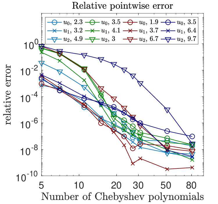
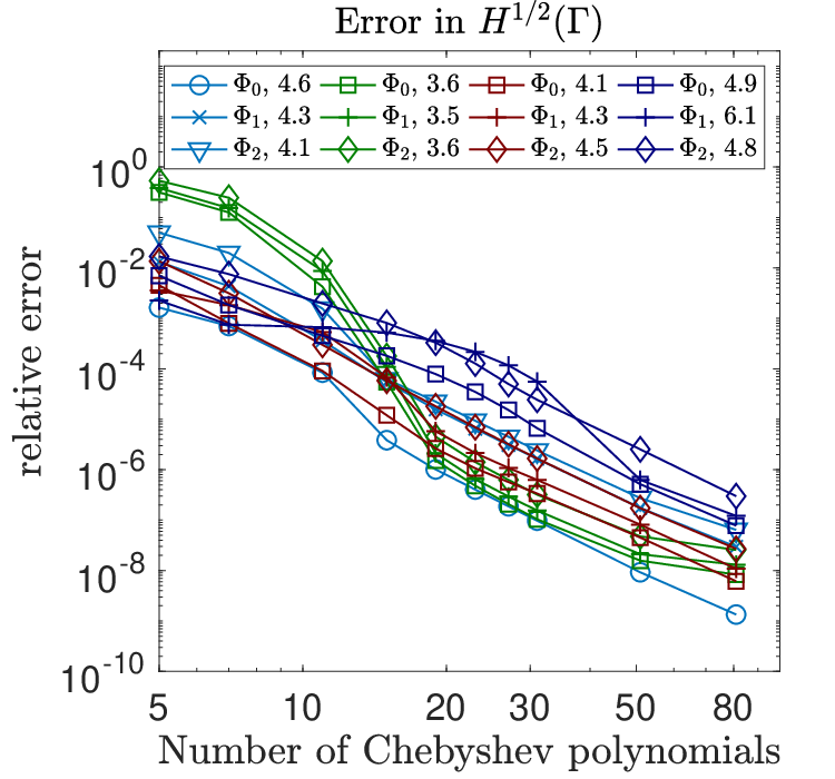
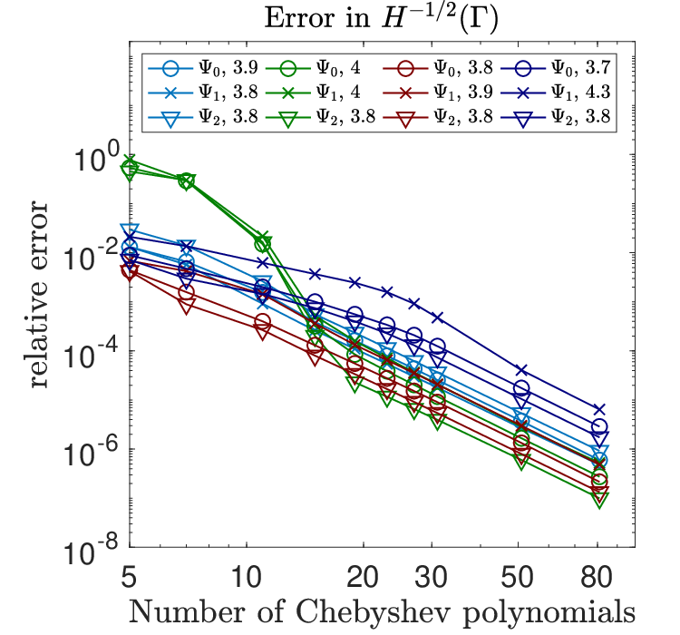
First, we show convergence results for the non-conforming spectral discretization presented in Section 4.1. Although we are using a spectral non-conforming discretization with Chebyshev polynomials, convergence rates are not expected to be exponential. This is related to the regularity of solutions of Helmholtz transmission problems in non-smooth domains [14]. Our aim is to show that we still obtain high-order convergence rates with accurate solutions using only a relatively small number of degrees of freedom.

We solve Problem 2.2 for a domain given by the circle with radius r=0.5r=0.5 with two subdomains (see Figure 2(a)). The volume problem to be solved by the MTF in these examples corresponds to

{−Δ​U+si2​U=0in ​Ωi,i=0,1,2,⟦γ​U⟧0​i=−γ​Uinc|Γ0​i,i=1,2,⟦γ​U⟧12=0,⟦γ​U⟧21=0,\left\{\begin{array}[]{rcll}-\Delta U+s_{i}^{2}U&=&0&\text{in }\Omega_{i},\ i=0,1,2,\\ \llbracket{\gamma U}\rrbracket_{0i}&=&-\gamma U^{\text{inc}}|_{\Gamma_{0i}},&\quad\qquad i=1,2,\\ \llbracket{\gamma U}\rrbracket_{12}&=&0,&\\ \llbracket{\gamma U}\rrbracket_{21}&=&0,&\end{array}\right. (47)
Table 2: Parameters used in Section 6.1. Convergence results are shown in Figure 3.
s0s_{0} s1s_{1} s2s_{2} UincU^{\text{inc}} 𝒅\bm{d}
Example A (blue) −i-i −2​i-2i −4​i-4i exp(−s0𝒙⋅𝒅)\exp(-s_{0}\bm{x}\cdot\bm{d}) (0,−1)(0,-1)
Example B (green) 1−i1-i 2−2​i2-2i 4−4​i4-4i exp(−s0𝒙⋅𝒅)\exp(-s_{0}\bm{x}\cdot\bm{d}) (0,−1)(0,-1)
Example C (brown) 1−i1-i 10−10​i10-10i 20−20​i20-20i exp(−s0𝒙⋅𝒅)\exp(-s_{0}\bm{x}\cdot\bm{d}) (0,−1)(0,-1)
Example D (purple) 1−i1-i 10−10​i10-10i 100−100​i100-100i exp(−s0𝒙⋅𝒅)\exp(-s_{0}\bm{x}\cdot\bm{d}) (0,−1)(0,-1)

The parameters employed are shown in Table 2. Errors are measured with respect to a highly resolved solution. Convergence results are displayed in Figure 3. Different values of ss are used in order to study errors for different problems. As expected, Galerkin solutions initially converge spectrally and then reach a finite order convergence rate due to the non-smoothness of the domains. Small errors are obtained with few degrees of freedom, which is adequate for coupling with BDF2 and two-stage RadauIIA CQ methods. For LobattoIIIc, a higher number of degrees of freedom is required to match its high order convergence in time. In order to study convergence of CQ time-stepping, we fix a high polynomial degree to suppress errors due to the Laplace domain solver.
Refer to caption
(a) Dirichlet trace errors
Refer to caption
(b) Neumann trace errors
Refer to caption
(c) Field errors
Figure 3: Different relative error norms for the two subdomains case (see Figure 2(a)) measured with respect to a highly resolved solution. Legends show estimated orders of convergence obtained by means of least squares fittings.

6.2 Manufactured time-domain solutions with no triple points

We now analyze our time-domain CQ-MTF by considering the case of a single domain, i.e. no triple points. The domain Ω\Omega consists of a circle of radius r=0.5r=0.5. We construct transmission conditions such that the exterior solution is zero whereas the interior one corresponds to

u1(𝒙,t):=f(c1t−tl​a​g−𝒙⋅𝒅),f(t):=sin(ωt)η(t,0.2,2),i=1,2,u_{1}(\bm{x},t):=f(c_{1}t-t_{lag}-\bm{x}\cdot\bm{d}),\quad f(t):=\sin(\omega t)\eta(t,0.2,2),\quad i=1,2, (48)
c0c_{0} c1c_{1} ω\omega TT tlagt_{\text{lag}} 𝒅\bm{d} NchebN_{\text{cheb}}
11 0.50.5 11 55 0.50.5 (1,0)(1,0) 4040
Table 3: Parameters used in Section 6.2.

where the parameters used are provided in Table 3. Therein, η\eta is a smooth version of the Heaviside function defined as

η⁡(t,t0,t1):={00≤t<t0,1−exp⁡(2e−1/ττ−1),τ=t−t0t1−t0,t0<t<t1,1t>t1.\eta(t,t_{0},t_{1}):=\left\{\begin{array}[]{cl}0&0\leq t<t_{0},\\ 1-\exp\left(\dfrac{2e^{-1/\tau}}{\tau-1}\right),\ \tau=\dfrac{t-t_{0}}{t_{1}-t_{0}},&t_{0}<t<t_{1},\\ 1&t>t_{1}.\\ \end{array}\right. (49)

Convergence results for BDF2 and Runge-Kutta CQ methods are displayed in Figure 4. Classical orders of convergence are restricted to the exterior domain (Fig. 4(c)), whereas for interior ones, CQ methods suffer from reduced convergence rates (Fig. 4(a) 4(b)). We observe that the three implemented methods share the same convergence rates for Neumann traces. This is explained by the low temporal regularity of the solutions, as normally the methods would achieve different orders of convergence.

Refer to caption
(a) Dirichlet trace errors
Refer to caption
(b) Neumann trace errors
Refer to caption
(c) Field errors
Figure 4: Relative errors for the transmission problem measured with respect to the analytical solution. Errors are computed as explained in (42) and (43). Legends show the estimated order of convergence obtained by means of least-squares fittings.

6.3 Manufactured time-domain solutions with artificial subdomains

We now validate the use of CQ-MTF by considering the case of artificial subdomains. The domain Ω\Omega consists in a circle of radius r=0.5r=0.5 separated into two subdomains Ω1\Omega_{1} and Ω2\Omega_{2} –left and right semicircles, respectively in Figure 2(a). We use the same manufactured solutions from Section 6.2. As the physical parameters of both subdomains are identical, the only difference from the case in Section 6.2 is the presence of an artificial triple point.

c0c_{0} c1c_{1} c2c_{2} ω\omega TT tlagt_{\text{lag}} 𝒅\bm{d} NchebN_{\text{cheb}}
11 0.50.5 0.50.5 11 55 0.50.5 (1,0)(1,0) 4040
Table 4: Parameters used in Section 6.3.

Error convergence results for BDF2 and Runge-Kutta-based CQ (RadauIIa and LobattoIIIc) are shown in Figure 5. Only small differences can be pointed out with respect to the results of Section 6.2, in particular, for the convergence of Neumann traces as they appear to improve for RadauIIa. However, these results are not sufficient to state that increasing the number of subdomains artificially impacts the convergence of the method.

Refer to caption
(a) Dirichlet trace errors
Refer to caption
(b) Neumann trace errors
Refer to caption
(c) Field errors
Figure 5: Relative errors for the two artificial-subdomains case measured with respect to the analytical solution. Errors are computed as explained in (42) and (43). Legends show estimated order of convergence obtained by means of least squares fittings.

6.4 Incident plane wave over a circle with two subdomains

We now consider as incident field a plane wave coming from Ω0\Omega_{0}, defined as

uinc​(𝒙,t)=f⁡(c0​(t−tlag)−𝒙⋅𝐝),f⁡(t)=sin⁡(ω​t)​η​(t,0.2,2).u^{\text{inc}}(\bm{x},t)=f(c_{0}(t-t_{\text{lag}})-\bm{x}\cdot\mathbf{d}),\quad f(t)=\sin(\omega t)\eta(t,0.2,2). (50)

The domain is a circle of radius r=0.5r=0.5 divided into two subdomains from Figure 2(a), with parameters used are shown in Table 5.

c0c_{0} c1c_{1} c2c_{2} ω\omega TT tlagt_{\text{lag}} 𝒅\bm{d} NchebN_{\text{cheb}}
11 0.50.5 0.250.25 88 1010 0.50.5 (0.5,−0.5)(\sqrt{0.5},-\sqrt{0.5}) 8080
Table 5: Parameters used in Section 6.4.

Error convergence results with respect to a highly resolved solution for each subdomain are shown in Figure 6. We observe that the second order convergence for the BDF2 method is not achieved until a high number of timesteps is reached due to the highly oscillatory behavior of the incident field. Runge-Kutta methods show the expected order of convergence for Dirichlet traces and for the scattered field, having even better results for the case of RadauIIa. Neumann traces present a slower convergence, as in previous examples. This behaviour is related to the stage order of convergence in Runge-Kutta methods, which is the same for two-stages RadauIIa and three-stages LobattoIIIc (q=2q=2). Some snapshots of the solution are shown in Figure 7.

Refer to caption
(a) Dirichlet trace errors
Refer to caption
(b) Neumann trace errors
Refer to caption
(c) Field errors
Figure 6: Relative errors for the two subdomains case measured with respect to a highly resolved solution. Errors are computed as explained in (42) and (43). Legends show methods employed with estimated orders of convergence obtained by means of least squares fittings.
Refer to caption Refer to caption Refer to caption
Figure 7: Snapshots of the computed field from problem in Section 6.4 for the times t = 0, 1.25, 2.5, 3.75, 5, 6.25, 7.5, 8.75, 10.

6.5 Incident Plane Wave over a Square with Four Subdomains

In this experiment, the incident field is the same plane wave from (50) coming from Ω0\Omega_{0} with parameters used are tl​a​g=0.5,𝒅=(0.5,−0.5)t_{lag}=0.5,\ \bm{d}=(\sqrt{0.5},-\sqrt{0.5}) and ω=8.\omega=8. The domain is a square of side length a=1a=1 divided into four subdomains (see Figure 2(b) ). Wavespeeds on each subdomain are c0=1,c1=0.5,c2=0.25,c3=0.5,c4=0.25c_{0}=1,c_{1}=0.5,c_{2}=0.25,c_{3}=0.5,c_{4}=0.25.

Table 6: Parameters used in Section 6.5.
c0c_{0} c1c_{1} c2c_{2} c3c_{3} c4c_{4} ω\omega TT tlagt_{\text{lag}} 𝒅\bm{d} NchebN_{\text{cheb}}
11 0.50.5 0.250.25 0.50.5 0.250.25 88 1010 0.50.5 (0.5,−0.5)(\sqrt{0.5},-\sqrt{0.5}) 2020

Convergence results for each interface are shown in Figure 8. We observe a similar behaviour to the previous example, with slow convergence for the BDF2 method. Snapshots of the volume solution are displayed in Figure 9.

Refer to caption
(a) Dirichlet trace errors
Refer to caption
(b) Neumann trace errors
Refer to caption
(c) Field errors
Figure 8: Relative errors for the four subdomains case measured with respect to a highly resolved solution. Errors are computed as explained in (42) and (43). Legends indicate estimated order of convergence obtained by means of least squares fittings.
Refer to caption Refer to caption Refer to caption
Figure 9: Snapshots of the computed field from problem in Section 6.5 for times t = 0, 1.25, 2.5, 3.75, 5, 6.25, 7.5, 8.75, 10.0.

6.6 Incident plane wave over kite with two subdomains

For our last experiment, the incident field is the same plane wave from (50) coming from Ω0\Omega_{0}. The domain is a smooth kite parametrized as follows

(x⁡(t)y⁡(t))=(cos⁡(t)+0.65​cos⁡(2​t)sin⁡(t)),t∈[0,2​π]\begin{pmatrix}x(t)\\ y(t)\end{pmatrix}=\begin{pmatrix}\cos(t)+0.65\cos(2t)\\ \sin(t)\end{pmatrix},\quad t\in[0,2\pi] (51)

divided into two subdomains Ω1\Omega_{1} and Ω2\Omega_{2} (corresponding to upper and lower halves) with symmetry over the x−x-axis. Parameters used are shown in Table 7. Convergence results for each interface are shown in Figure 10. Snapshots of the volume solution are displayed in Figure 11.

Table 7: Parameters used in Section 6.6.
c0c_{0} c1c_{1} c2c_{2} ω\omega TT tlagt_{\text{lag}} 𝒅\bm{d} NchebN_{\text{cheb}}
11 0.50.5 0.250.25 88 1010 0.50.5 (1,0)(1,0) 8080
Refer to caption
(a) Dirichlet trace errors
Refer to caption
(b) Neumann trace errors
Refer to caption
(c) Field errors
Figure 10: Relative errors for the two subdomains case in a kite-shaped domain, measured with respect to a highly resolved solution. Errors are computed as explained in (42) and (43). Legends indicate estimated order of convergence obtained by means of least squares fittings.
Refer to caption Refer to caption Refer to caption
Figure 11: Snapshots of the computed field from problem in Section 6.6 for times t = 0.5, 1.5, 2.5, 3.5, 4.5, 5.5, 6.5, 7.5, 8.5.

7 Concluding remarks

We solve acoustic wave transmission problems in 2D over composite scatterers by means of CQ methods coupled to a non-conforming spectral Galerkin discretization in space. We showed that Runge-Kutta CQ constitutes an efficient and accurate method, preferable to multistep methods due to their higher order convergence rates. Although reduced order can be expected, this was only observed for the convergence of Neumann traces. For every example, convergence of two-stage Radau and three-stage Lobatto coincides for Neumann traces, which can be explained with the fact that both methods have exactly the same stage order q=2q=2.

The use of high-order spatial discretizations for frequency domain problems is mandatory in order to achieve accurate results and take advantage of the capabilities of Runge-Kutta methods. This is achieved in space via a non-conforming spectral Galerkin discretization. Chebyshev polynomials are also suitable functions for the framework of piecewise/broken Sobolev spaces defined over the boundary of each subdomain.

Future work will be focused on developing a convergence theory for this formulation. Although very important advances have been made in previous works in [16, 30, 31, 32], the current theoretical framework is well suited only for Galerkin-BEM on standard Sobolev spaces over the boundary of Lipschitz domains. Unfortunately, it is not clear how to extend this to piecewise or broken spaces considered for trial and test functions in the MTF, or even the Petrov-Galerkin formulation.

Acknowledgments

This research was funded by FONDECYT Regular 1171491.

References

  • [1] L. Banjai and C. Lubich. An error analysis of Runge–Kutta Convolution Quadrature. BIT Numerical Mathematics, 51(3):483–496, 2011.
  • [2] L. Banjai, C. Lubich, and J. M. Melenk. Runge–Kutta Convolution Quadrature for operators arising in Wave propagation. Numerische Mathematik, 119(1):1–20, 2011.
  • [3] L. Banjai, M. Messner, and M. Schanz. Runge–Kutta Convolution Quadrature for the Boundary Element Method. Computer methods in applied mechanics and engineering, 245:90–101, 2012.
  • [4] L. Banjai and S. Sauter. Rapid Solution of the Wave Equation in Unbounded Domains. SIAM Journal on Numerical Analysis, 47(1):227–249, 2008.
  • [5] L. Banjai and M. Schanz. Wave propagation problems treated with Convolution Quadrature and BEM. In Fast Boundary Element Methods in Engineering and Industrial Applications, pages 145–184. Springer, 2012.
  • [6] X. Claeys, R. Hiptmair, and C. Jerez-Hanckes. Multitrace Boundary Integral Equations. In Direct and inverse problems in wave propagation and applications, volume 14 of Radon Ser. Comput. Appl. Math., pages 51–100. De Gruyter, Berlin, 2013.
  • [7] X. Claeys, R. Hiptmair, C. Jerez-Hanckes, and S. Pintarelli. Novel Multi-Trace Boundary Integral Equations for Transmission Boundary Value Problems. In A. S. Fokas and B. Pelloni, editors, Unified Transform for Boundary Value Problems: Applications and Advances, pages 227–258. Philadelphia, SIAM, 2015.
  • [8] X. Claeys, R. Hiptmair, and E. Spindler. A second-kind Galerkin Boundary Element method for scattering at composite objects. BIT Numerical Mathematics, 55(1):33–57, 2015.
  • [9] P. J. Davies. A stability analysis of a time marching scheme for the general surface electric field integral equation. Applied Numerical Mathematics, 27(1):33–57, 1998.
  • [10] P. J. Davies and D. B. Duncan. Averaging techniques for time-marching schemes for retarded potential integral equations. Applied Numerical Mathematics, 23(3):291–310, 1997.
  • [11] P. J. Davies and D. B. Duncan. Stability and convergence of collocation schemes for retarded potential integral equations. SIAM Journal on Numerical Analysis, 42(3):1167–1188, 2004.
  • [12] P. J. Davies, D. B. Duncan, and B. Zubik-Kowal. The stability of numerical approximations of the time domain current induced on thin wire and strip antennas. Applied numerical mathematics, 55(1):48–68, 2005.
  • [13] S. Eberle, F. Florian, R. Hiptmair, and S. Sauter. A stable boundary integral formulation of an acoustic wave transmission problem with mixed boundary conditions. SIAM Journal on Mathematical Analysis, 53(2):1492–1508, 2021.
  • [14] P. Grisvard. Elliptic problems in nonsmooth domains. SIAM, 2011.
  • [15] M. Hassell and F.-J. Sayas. Convolution Quadrature for Wave simulations. In Numerical simulation in physics and engineering, pages 71–159. Springer, 2016.
  • [16] M. E. Hassell, T. Qiu, T. Sánchez-Vizuet, F.-J. Sayas, et al. A new and improved analysis of the time domain boundary integral operators for the acoustic wave equation. Journal of Integral Equations and Applications, 29(1):107–136, 2017.
  • [17] F. Henríquez and C. Jerez-Hanckes. Multiple Traces Formulation and Semi-Implicit Scheme for Modelling Biological Cells under Electrical Stimulation. ESAIM Mathematical Modelling and Numerical Analysis, 52(2):659–703, 2018.
  • [18] F. Henríquez, C. Jerez-Hanckes, and F. Altermatt. Boundary Integral Formulation and Semi-Implicit Scheme coupling for Modeling Cells under Electrical Stimulation. Numerische Mathematik, 136:101–145, 2017.
  • [19] R. Hiptmair and C. Jerez-Hanckes. Multiple Traces Boundary Integral Formulation for Helmholtz Transmission Problems. Advances in Computational Mathematics, 37(1):39–91, 2012.
  • [20] C. Jerez-Hanckes, S. Nicaise, and C. Urzúa-Torres. Fast spectral galerkin method for logarithmic singular equations on a segment. Journal of Computational Mathematics, 36(1):128–158, 2018.
  • [21] C. Jerez-Hanckes, C. Pérez-Arancibia, and C. Turc. Multitrace/singletrace formulations and Domain Decomposition Methods for the solution of Helmholtz transmission problems for bounded composite scatterers. Journal of Computational Physics, 350:343–360, 2017.
  • [22] C. Jerez-Hanckes, J. Pinto, and S. Tournier. Local multiple traces formulation for high-frequency scattering problems. Journal of Computational and Applied Mathematics, 289:306–321, 2015.
  • [23] C. Jerez-Hanckes, J. Pinto, and S. Tournier. Local Multiple Traces Formulation for High-Frequency Scattering Problems by Spectral Elements. In Scientific Computing in Electrical Engineering, pages 73–82. Springer, 2016.
  • [24] M. Lopez-Fernandez and S. Sauter. Generalized Convolution Quadrature with variable time stepping. IMA Journal of Numerical Analysis, 33(4):1156–1175, 2013.
  • [25] M. Lopez-Fernandez and S. Sauter. Generalized Convolution Quadrature based on Runge-Kutta methods. Numerische Mathematik, 133(4):743–779, 2016.
  • [26] C. Lubich. Convolution Quadrature and Discretized Operational Calculus. I. Numerische Mathematik, 52(2):129–145, 1988.
  • [27] C. Lubich. Convolution Quadrature and Discretized Operational Calculus. II. Numerische Mathematik, 52(4):413–425, 1988.
  • [28] C. Lubich and A. Ostermann. Runge-Kutta Methods for Parabolic Equations and Convolution Quadrature. Mathematics of Computation, 60(201):105–131, 1993.
  • [29] W. C. H. McLean. Strongly Elliptic systems and Boundary Integral Equations. Cambridge university press, 2000.
  • [30] T. Qiu. Time Domain Boundary Integral Equation methods in Acoustics, Heat diffusion and Electromagnetism. PhD thesis, University of Delaware, 2016.
  • [31] T. Qiu and F.-J. Sayas. The Costabel-Stephan system of Boundary Integral Equations in the Time Domain. Mathematics of Computation, 85(301):2341–2364, 2016.
  • [32] D.-I. A. Rieder. Convolution Quadrature and Boundary Element Methods in wave propagation. PhD thesis, Technische Universität Wien, 2017.
  • [33] F.-J. Sayas. Retarded Potentials and Time Domain Boundary Integral Equations: A Road Map, volume 50. Springer, 2016.
  • [34] O. Steinbach. Numerical approximation methods for elliptic boundary value problems: finite and boundary elements. Springer Science & Business Media, 2007.
  • [35] L. N. Trefethen. Approximation theory and approximation practice, volume 128. Siam, 2013.
  • [36] G. Wanner and E. Hairer. Solving ordinary differential equations II. Springer Berlin Heidelberg, 1996.
  • [37] G. Wanner, E. Hairer, and S. P. Norsett. Solving ordinary differential equations I. Springer Berlin Heidelberg, 1993.