Quantum communication capacity transition of complex quantum networks
Abstract
Quantum network is the key to enable distributed quantum information processing. As the single-link communication rate decays exponentially with the distance, to enable reliable end-to-end quantum communication, the number of nodes needs to grow with the network scale. For highly connected networks, we identify a threshold transition in the capacity as the density of network nodes increases—below a critical density, the rate is almost zero, while above the threshold the rate increases linearly with the density. Surprisingly, above the threshold the typical communication capacity between two nodes is independent of the distance between them, due to multi-path routing enabled by the quantum network. In contrast, for less connected networks such as scale-free networks, the end-to-end capacity saturates to constants as the number of nodes increases, and always decays with the distance. Our results are based on capacity evaluations, therefore the minimum density requirement for an appreciable capacity applies to any general protocols of quantum networks.
I Introduction
Quantum information (QI) science has brought advantages in various applications Shor 1997; Giovannetti et al. 2004; Bennett et al. 2002; Gisin and Thew 2007. To unleash the full power of QI processing in distributed tasks Lynch 1996; Andrews 2000, a quantum network (QN) Kimble 2008; Biamonte et al. 2019; Wehner et al. 2018; Kozlowski and Wehner 2019; Miguel-Ramiro et al. 2020 aiming at entanglement distribution and QI transmission is the key.
The Internet is mainly built upon fiber networks, with photons as the information carrier. Similarly, photons as the only known “flying qubits” will likely be the information carrier in a QN. In both cases, channel loss is the major challenge to communication. Therefore, networking protocols that make use of intermediate nodes or repeaters are important for both. Unlike classical information, QI cannot be simply cloned and amplified, and therefore increasing the number of nodes, even repeater nodes Briegel et al. 1998; Jiang et al. 2009; Sangouard et al. 2011; Munro et al. 2015; Muralidharan et al. 2016; Dias and Ralph 2017; Muralidharan et al. 2018; Furrer and Munro 2018; Dias et al. 2020; Seshadreesan et al. 2020; Goodenough et al. 2020, is costly. In this regard, a key question for designing a QN is to understand the trade-off between the density of nodes and the entanglement distribution rate: how many nodes are necessary to guarantee reliable QI transmission between multiple users in a fixed region?
The answer not only depends on the overall distances between the users, but also on the topology of the QN to be built Acín et al. 2007. As it is likely that well-developed classical fiber networks can be adopted as the base of QN s, Ref. Brito et al. 2020 developed a model for QN on the the probabilistic transmission of single photons and took a classical network science approach to study its connectivity by the giant component. However, for QN s exploiting quantum technologies such as quantum error correction Calderbank and Shor 1996 and non-classical state generation Caves 1981; Gottesman et al. 2001, the semi-classical approach has a limited implication. In particular, Ref. Brito et al. 2020’s critical density highly depends on the number of repetitions of each channel use and thus blurs the essential constraints. More recently, Refs. Rabbie et al. 2020; coutinho2021 considered effects from repeater nodes. As the results rely on specific protocols, the fundamental limits of the trade-off remains unclear. We address the same question with a full QI approach based on the fundamental limits pirandola2009; Takeoka et al. 2014; Pirandola et al. 2017; Pirandola 2019; Azuma et al. 2016, and obtain a minimum density requirement that generally applies to any protocols.
As the exact architecture and protocols of QN s are unclear, we take the information-theoretical approach and evaluate the end-to-end capacity Pirandola 2019 of QI transmission. To account for different possibilities of the future QN s, we consider typical types of network models Pastor-Satorras and Vespignani 2007, based on the Waxman networks Waxman 1988; Lakhina et al. 2003, Erdős-Rényi model and scale-free networks Barabási and Albert 1999; Yook et al. 2002. Our results provide an upper bound to characterize the quantum capacity of QN s and the analysis applies to all kinds of quantum communication. In Waxman and Erdős-Rényi QN s, the ensemble-averaged capacity abruptly transits from almost zero to nonzero values at a critical density of nodes. Above the threshold, it grows with the density linearly, at a rate depending on the statistical properties of the QN. Surprisingly, in this region the end-to-end capacity typically does not depend on the distance between the two end nodes, due to the multi-path routing enabled by the coordination of the entire QN. In scale-free QN s, the ensemble-averaged capacity saturates to a constant depending on the scale of the network as the density of nodes increases, due to the limited connectivity in the network that prevents efficient multi-path routing.
II Model of QN s
The skeleton of a QN can be described by a graph, with vertices being the network nodes and edges representing the transmission links Zhang and Zhuang 2020. As nodes are located geographically, we can assign a 2-D coordinate to each node. The transmission link along each edge is modeled as a bosonic pure loss channel, with a transmissivity for fiber length at a state-of-the-art rate per kilometer (km). For simplicity, we assume that for each edge, the fiber length and the geographical distance are identical.
With the transmission links on each edge defined, one needs to specify the graph structure—the coordinates and connections of the vertices—to specify the QN. Without loss of generality, we choose the coordinates of the nodes uniformly random in a square , with an area of .
In the random Waxman model Waxman 1988; Lakhina et al. 2003, each pair of nodes is connected with a probability decaying exponentially with the distance. Here is the maximum possible distance in a square; the constant controls the typical fiber length and is fixed so that km to model the U.S. fiber-optics networks Lakhina et al. 2003. It is worthy to point out that Ref. Brito et al. 2020 adopted the same Waxman QN s. In the scale-free model Yook et al. 2002, the network is built up dynamically: when each node is being added, it is connected to nodes out of all the previous added nodes. The probability of node being connected to node is proportional to the current degree and inversely proportional to the distance , i.e., in contrast to the Waxman model’s exponential decay with distance.
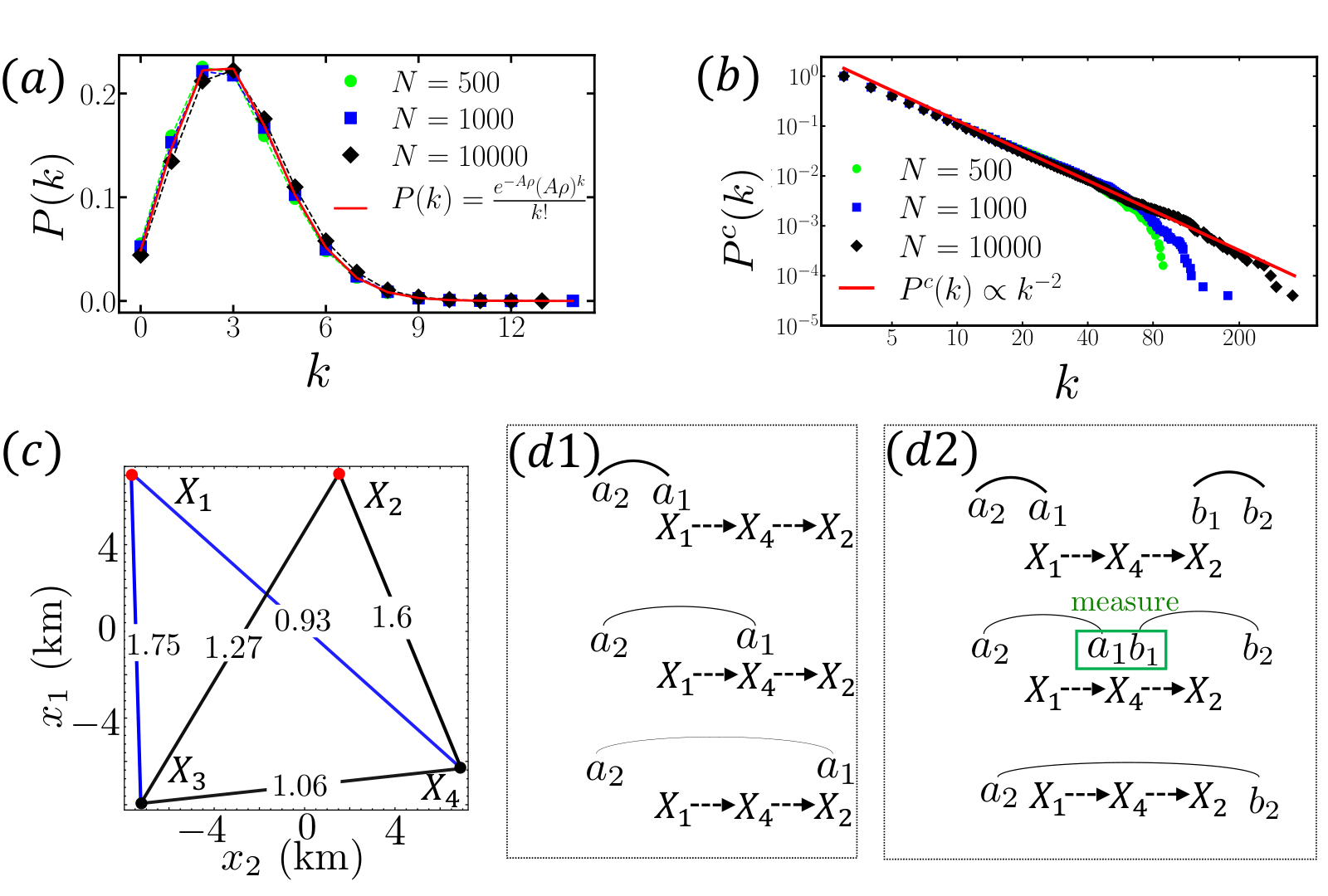

To obtain a direct impression, we visualize the two models in Fig. 2 (a) and Fig. 4 (a) respectively. Immediate differences in the connectivity can be seen, e.g. by comparing Fig. 2 (a2) and Fig. 4 (a1): for the same nodes in a region of scale km, the Waxman model is much more connected and homogeneous, while the scale-free model is less connected and heterogeneous. These differences can be captured by their statistical properties. As shown in Fig. 1(a)(b), the Waxman QN model has a Poisson degree distribution and the average degree grows with the number of nodes linearly poisson; while the scale-free QN model has a long-tailed power-law degree distribution and a bounded average of . It is also worthy mentioning that the Waxman model has a percolation phase transition (see Appendix A), where the percentage of the giant component of the graph increases sharply from close to zero to unity as the density increases above a critical value of . However, we show that this necessary condition is far from being sufficient.
While we base our QN models on the Internet, a QN will be majorly different from Internet. In particular, classical repeaters Mukherjee 2000 are not counted as network nodes in the study of Internet Pastor-Satorras and Vespignani 2007, as they are universally deployed and cheap. In contrast, quantum repeaters are nontrivial and therefore directly considered as network nodes in this study. In this regard, the Waxman model’s exponential decay of long direct links will be more likely for QN s. However, our goal is not to determine which model can better represent a QN, an emerging technology, but to characterize each model in terms of quantum communications.
III Protocols and capacity formula
To distribute entanglement between two nodes and in a QN, the nodes can transmit quantum states between all links and perform two-way classical communication in combination of local operations at each node. To begin with, let’s consider an instance of a four-node network in Fig. 1(c). In a single-path routing strategy, one can choose a path from to (e.g. , , or ) and utilize all the channels along the path once to distribute the entanglement. With the path fixed, one can either perform direct communication or adopt entanglement swap Zukowski et al. 1993, as shown in Fig. 1(d). A more efficient approach is to adopt multi-path routing. For example, nodes and in Fig. 1(c) can utilize multiple non-overlapping paths simultaneously ( and ) and achieve a better performance.
As protocols vary, to obtain universal results, we consider the ultimate achievable entanglement distribution rate among all protocols Pirandola et al. 2017; Pirandola 2019. In contrast to classical communication GiovannettiV2014; Giovannetti et al. 2004, QI transmission rate for each edge is fundamentally limited by the channel loss to be
| (1) |
regardless of the energy, where is the channel loss Pirandola et al. 2017. To characterize the importance of a single node, we define the node capacity , as the sum of the edge capacities.
Consider the graph with edge capacities as the weights (e.g. Fig. 1(c)), the problem of solving the end-to-end capacity is reduced to solving the minimum cut Pirandola 2019. Let’s first introduce a cut between two nodes and as the set of edges such that their deletion will disconnect the two nodes. For example, in Fig. 1(c), the blue part indicates a cut for and . Then the capacity between end nodes and is given by the “edge connectivity” between them Pirandola 2019
| (2) |
To obtain further insights, we derive an upper bound of the end-to-end capacity by the node capacities of the two end nodes, as one can always choose the cut that consists of all edges connected to one of the end nodes.
We take a statistical approach and evaluate the average end-to-end capacity in an ensemble of network models, where the average is over the choices of the end nodes , and the random realization of the network, with fixed numbers of nodes and scale . In this regard,
| (3) |
upper bounded by the ensemble-averaged node capacity. Compared to the edge connectivity approach based on probabilistic single-photon transmission in Ref. Brito et al. 2020, our quantum capacity approach applies to all protocols and reveals essential features of a network.
IV Rate transition of Waxman QN s
To study Waxman QN s, we first fix the scale km and vary the number of nodes . In Fig. 2 (b), we plot the end-to-end capacity of random pairs vs. the graph distance (the shortest path length) between them. When the number of nodes is small (e.g. Fig. 2 (b1)), the capacity decays with the graph distance drastically; while surprisingly, when the number of nodes becomes larger (e.g. Fig. 2 (b2)), the capacity is almost independent of the graph distance patil2020. This is due to the effect of multi-path routing—the number of possible paths increases significantly with distance when the nodes are dense.

To systematically evaluate the transition in the end-to-end capacity, we evaluate the ensemble-averaged capacity for different values of and . We expect the density of nodes to be the crucial parameter. Indeed, we can show that when is large, the ensemble-averaged node capacity , as the upper bound in Ineq. (3), is linear in density with the coefficient (see Appendix C).
In Fig. 3 (a), we plot the average capacity vs the node density for different system size . Overall, for a fixed density , the capacity converges as the scale increases. When the density is small, the capacity is mostly close to zero (see Appendix B); As the density increases, we see a sudden transition from almost zero capacity to capacity at a critical density. The transition happens at around corresponding to a density , which is much larger than the giant component transition and the result from Ref. Brito et al. 2020.
After this transition, the average capacity increases linearly with node density , approaching the upper bound (dark green line). The reason of the convergence can be observed from Fig. 2 (a): when the connectivity is high, the minimum cut (blue edges) becomes a cut formed by all the edges connecting to one of the end points. To be more quantitative, we calculate the ratio of the edges in the minimum cut that contain at least one end node. As shown in Fig. 3 (b), the ratio transits from close to zero to unity at the same time as the end-to-end capacities approach the upper bounds. In fact, we find that a shifted upper bound fits the overall numerical results well, as shown by the green dashed line in Fig. 3(a).
Note that Ref. Brito et al. 2020’s critical density depends on the protocol parameters—e.g. the number of repetition for each link; therefore the value of their critical density is not an essential characterization of the QN. Their results have to obey the constraint in our paper, as any protocol has its rate bounded by the capacity. We can confirm as follows: as they consider repeated use of each channel to successfully establish one single Bell pair, the end-to-end capacity per channel use in their protocol is merely for density , which is in fact within the vanishing capacity region in our results.
V Rate saturation of scale-free QN s
Now we switch the focus to scale-free QN s (see Fig. 4). Similarly, we evaluate the end-to-end capacity for the same set of choices of and . In Fig. 5 (a), the ensemble-averaged capacity grows as increases and saturates to a constant dependent on the scale of the network. This is due to the limited degree of scale-free networks, which constrains the upper bound of the node capacity to be bounded by a constant and dependent on (see Appendix E). As we can see in Fig. 5 (b), the ratio of edges of end points being in the minimum cut is now determined by the network scale, and gets close to unity when the network is small. Indeed, in Fig. 5 (c) we see the gap between the saturated capacity and the upper bound from node capacity is small for small , while larger with increasing. Overall, the capacity decays with exponentially, even when the number of nodes is large.
In additional to the saturation of capacity, the graph-distance-independence of the capacity is absent for scale-free QN s. In Fig. 4 (b), regardless of the capacity being large or small, there is a sharp decrease of the end-to-end capacity as the graph distance increases, in contrast to the Waxman QN s in Fig. 2 (b). This is due to the lack of multi-path routing, constrained by the connectivity of the scale-free networks. Indeed, we can find the average clustering coefficient decaying with the system size, instead of saturating to constants with number of nodes in the Waxman case (see Appendix A).
VI Rate transition of Erdős-Rényi QN s
We also extend our analyses to the Erdős-Rényi model, a network model with uniform edge connection probability . To compare with the Waxman model, we match the number of edges in Erdős-Rényi model to the Waxman model with same and , via choosing a proper . The corresponding degree distribution is binomial (see Appendix A).
We evaluate the transition of average end-to-end capacity with node density in Fig. 3(c), and identify similar trend to the Waxman model: when is large, grows linearly with ; while when is small, there is still a sharp decrease in the capacity. While in the Waxman model, the capacity agrees among different in the linear transition, Erdős-Rényi model shows a clear dependence on , and thus on the connection probability . We can also explore further the dependence on through the upper bound of node capacity in Eq. (3). where (see Appendix D). We can directly see the dependence of on connection probability from the asymptotic upper bound and we show them in Fig. 3(c).
VII Conclusion and discussions
In this paper, we examine the end-to-end quantum communication capacity in Waxman, Erdős-Rényi QN s and scale-free QN s. Our results provide guidance on the design of QN infrastructure, as the capacity places an achievable upper bound on rates of quantum communication protocols.
In particular, our results suggest that when the connectivity of the QN is high (like in the Waxman case), multi-path routing will enable reliable quantum communication. On the practical side, considering that quantum repeaters might be as costly and expensive as user nodes, this indicates that at a moderate metropolitan scale where users are dense and direct links are possible, it might be better to simply build more direct links between the users and utilize the multi-path routing for reliable quantum communication.
Our results are based on network capacity results and therefore reveals essential property of a QN, independent on the protocol. We reveal more detailed properties of QN s, other than the simple connectivity properties in Ref. Brito et al. 2020. Our results address the entanglement generation capacity, which is the most relevant quantity in a QN. In particular, our results allow unlimited two-way classical communication (via an underlying classical network) as assistance in the entanglement generation process. Ref. Brito et al. 2020 limits the protocols to be at a single photon level, and is strongly dependent on the specific protocol parameters to generate entanglement. The density of nodes to guarantee reliable communication would depend on the exact meaning of reliable communication, however, a network above the threshold we identified is preferable as the capacity starts to become distance-independent.
Acknowledgements.
This research is supported by Defense Advanced Research Projects Agency (DARPA) under Young Faculty Award (YFA) Grant No. N660012014029, National Science Foundation (NSF) Engineering Research Center for Quantum Networks Grant No. 1941583. Q.Z. also acknowledges Craig M. Berge Dean’s Faculty Fellowship of University of Arizona.Appendix A Basic properties networks.
As shown in Fig. 7, in the Waxman model, the average degree of the nodes increases with the number of nodes linearly, at a rate depending on the scale ; In the scale-free network, the average degree saturates to as the number of nodes increases. Here is the number of edges brought by the addition of each single node.
We plot the degree distribution of Erdős Rényi model and mean degree in Fig. 7.
The Waxman model has a giant component transition as the density of nodes increases. As shown in Fig. 8(a), the ratio of the size of the largest connected component over the total number of nodes increases from close to zero to unity abruptly at a density of . The transition becomes sharper as the number of nodes increase.
To understand the connectivity of the networks, we plot the clustering coefficient’s dependence network parameters. For a single node, the single-node local clustering coefficient identifies the existence of connections between its neighbors . Here is number of triangles that is attached to the node . We can define the graph clustering coefficient by averaging over all nodes. For Waxman networks, converging to a constant dependent on as the number of nodes increases, as shown in Fig. 8(b). While for the scale-free networks, decays to zero as the number of nodes increases, as shown in Fig. 8(c).
Appendix B Additional data for the end-to-end capacity
We provide additional data of the numerical calculations. First, we show the distribution of the end-to-end capacity between random pairs of nodes in each ensemble of networks. Fig. 10 shows the Waxman case, corresponding to Fig. 2(b1)-(b5); while Fig. 10 shows the scale-free case, corresponding to Fig. 4(b1)(b2) of the main paper. The average of the data utilized here gives the red curves in the corresponding plots of the main paper, which are also shown as red curves in these plots.


Next, we present an in-depth analyses of Fig. 3 in the main paper. Fig. 11(a) shows each curve of capacity vs. number of nodes for different scales individually, without collapsing everything in plotting with density. In the main paper, we do not show the long tails, as these tails are mainly due to rare cases of random pairs of nodes lying very close to each other. Indeed, if we plot the median instead of the mean, as shown in Fig. 13, these long tails are not present and we see a clear sharp drop. To avoid burying the main take-away in such technical details, we do not present the entire data in the main paper. Here we also evaluated the exact upper bound from Eq. (5) for each curve, which converges to the asymptotic results shown in the main paper (see Fig. 13 for details of the convergence). In Fig. 11 (b), we calculate the critical number for , which is much larger than the giant component transition point or the results from Ref. Brito et al. 2020. We can also solve in Eq. (5) to obtain a lower bound estimate on , which works well when is large as shown in Fig. 11(c). In Fig. 11(d), we plot the capacity in linear scale to show the deviations between the actual capacities and the upper bounds in more detail. The major reason for the deviation at large and high density is due to the second inequality of Ineq. (3) of the main paper, which we also print here
| (4) |
as interchanging the order of ensemble averaging and minimization is not tight.

Appendix C Derivation of the asymptotic results for Waxman model
Due to the independence between the edges between nodes, we have
| (5) | ||||
| (6) | ||||
| (7) | ||||
| (8) | ||||
| (9) | ||||
| (10) | ||||
| (11) |
Inputting and we have the asymptotic expansion of
| (12) | ||||
| (13) |
In Fig. 13, we compare the asymptotic results with the exact numerical integration in Eq. (5). A good convergence towards the asymptotic result is found with the increasing scale .
Appendix D Derivation of node capacity in Erdős Rényi models
| (14) |
Appendix E Derivation of the asymptotic results for scale-free model
Considering the on average neighbours as independent, the ensemble-averaged node capacity is
| (15) | ||||
| (16) |
where the normalization constant
| (17) |
The inside the integral now denotes average over the degree distribution of neighbours, conditioned on the neighbour being at . We can approximate the distribution of the degree as independent of the distance to node , then , where is a constant and is an arbitrary function of . We can cancel out the constant and equivalently calculate
| (18) | ||||
| (19) |
The above integral can be numerically calculated. It is clear that does not grow with the number of nodes , as is now a constant.
References
- Shor (1997) P. Shor, Polynomial-time algorithms for prime factorization and discrete logarithms on a quantum computer, SIAM J. Comput. 26, 1484 (1997).
- Giovannetti et al. (2004) V. Giovannetti, S. Guha, S. Lloyd, L. Maccone, J. H. Shapiro, and H. P. Yuen, Classical capacity of the lossy bosonic channel: The exact solution, Phys. Rev. Lett. 92, 027902 (2004).
- Bennett et al. (2002) C. Bennett, P. Shor, J. Smolin, and A. Thapliyal, Entanglement-assisted capacity of a quantum channel and the reverse shannon theorem, IEEE Trans. Inf. Theory 48, 2637 (2002).
- Gisin and Thew (2007) N. Gisin and R. Thew, Quantum communication, Nat. Photonics 1, 165 (2007).
- Lynch (1996) N. A. Lynch, Distributed algorithms (Elsevier, 1996).
- Andrews (2000) G. R. Andrews, Foundations of multithreaded, parallel, and distributed programming, Vol. 11 (Addison-Wesley Reading, 2000).
- Kimble (2008) H. J. Kimble, The quantum internet, Nature 453, 1023 (2008).
- Biamonte et al. (2019) J. Biamonte, M. Faccin, and M. De Domenico, Complex networks from classical to quantum, Commun. Phys. 2, 53 (2019).
- Wehner et al. (2018) S. Wehner, D. Elkouss, and R. Hanson, Quantum internet: A vision for the road ahead, Science 362 (2018).
- Kozlowski and Wehner (2019) W. Kozlowski and S. Wehner, Towards large-scale quantum networks, in Proceedings of the Sixth Annual ACM International Conference on Nanoscale Computing and Communication (2019) pp. 1–7.
- Miguel-Ramiro et al. (2020) J. Miguel-Ramiro, A. Pirker, and W. Dür, Genuine quantum networks: superposed tasks and addressing, arXiv:2005.00020 (2020).
- Briegel et al. (1998) H.-J. Briegel, W. Dür, J. I. Cirac, and P. Zoller, Quantum repeaters: the role of imperfect local operations in quantum communication, Phys. Rev. Lett. 81, 5932 (1998).
- Jiang et al. (2009) L. Jiang, J. M. Taylor, K. Nemoto, W. J. Munro, R. Van Meter, and M. D. Lukin, Quantum repeater with encoding, Phys. Rev. A 79, 032325 (2009).
- Sangouard et al. (2011) N. Sangouard, C. Simon, H. De Riedmatten, and N. Gisin, Quantum repeaters based on atomic ensembles and linear optics, Rev. Mod. Phys. 83, 33 (2011).
- Munro et al. (2015) W. J. Munro, K. Azuma, K. Tamaki, and K. Nemoto, Inside quantum repeaters, IEEE Journal of Selected Topics in Quantum Electron. 21, 78 (2015).
- Muralidharan et al. (2016) S. Muralidharan, L. Li, J. Kim, N. Lütkenhaus, M. D. Lukin, and L. Jiang, Optimal architectures for long distance quantum communication, Sci. Rep. 6, 20463 (2016).
- Dias and Ralph (2017) J. Dias and T. C. Ralph, Quantum repeaters using continuous-variable teleportation, Phys. Rev. A 95, 022312 (2017).
- Muralidharan et al. (2018) S. Muralidharan, C.-L. Zou, L. Li, and L. Jiang, One-way quantum repeaters with quantum reed-solomon codes, Phys. Rev. A 97, 052316 (2018).
- Furrer and Munro (2018) F. Furrer and W. J. Munro, Repeaters for continuous-variable quantum communication, Phys. Rev. A 98, 032335 (2018).
- Dias et al. (2020) J. Dias, N. Hosseinidehaj, and T. C. Ralph, Quantum repeater for continuous variable entanglement distribution, arXiv:2004.06345 (2020).
- Seshadreesan et al. (2020) K. P. Seshadreesan, H. Krovi, and S. Guha, Continuous-variable quantum repeater based on quantum scissors and mode multiplexing, Phys. Rev. Research 2, 013310 (2020).
- Goodenough et al. (2020) K. Goodenough, D. Elkouss, and S. Wehner, Optimising repeater schemes for the quantum internet, arXiv:2006.12221 (2020).
- Acín et al. (2007) A. Acín, J. I. Cirac, and M. Lewenstein, Entanglement percolation in quantum networks, Nat. Phys. 3, 256 (2007).
- Brito et al. (2020) S. Brito, A. Canabarro, R. Chaves, and D. Cavalcanti, Statistical properties of the quantum internet, Phys. Rev. Lett. 124, 210501 (2020).
- Calderbank and Shor (1996) A. R. Calderbank and P. W. Shor, Good quantum error-correcting codes exist, Phys. Rev. A 54, 1098 (1996).
- Caves (1981) C. M. Caves, Quantum-mechanical noise in an interferometer, Phys. Rev. D 23, 1693 (1981).
- Gottesman et al. (2001) D. Gottesman, A. Kitaev, and J. Preskill, Encoding a qubit in an oscillator, Phys. Rev. A 64, 012310 (2001).
- (28) B. C. Coutinho, W. J. Munro, K. Nemoto and Y. Omar, Robustness of Noisy Quantum Networks, arXiv:2103.03266 (2021)
- Rabbie et al. (2020) J. Rabbie, K. Chakraborty, G. Avis, and S. Wehner, Designing quantum networks using preexisting infrastructure, arXiv:2005.14715 (2020).
- (30) S. Pirandola, R. García-Patrón, S. L. Braunstein, and S. Lloyd, Direct and reverse secret-key capacities of aquantum channel, Phys. Rev. Lett.102, 050503 (2009).
- Takeoka et al. (2014) M. Takeoka, S. Guha, and M. M. Wilde, Fundamental rate-loss tradeoff for optical quantum key distribution, Nat. Commun. 5, 5235 (2014).
- Pirandola et al. (2017) S. Pirandola, R. Laurenza, C. Ottaviani, and L. Banchi, Fundamental limits of repeaterless quantum communications, Nat. Commun. 8, 15043 (2017).
- Pirandola (2019) S. Pirandola, End-to-end capacities of a quantum communication network, Commun. Phys 2, 51 (2019); See also arXiv:1601.00966 (2016).
- Azuma et al. (2016) K. Azuma, A. Mizutani, and H.-K. Lo, Fundamental rate-loss trade-off for the quantum internet, Nat. Commun. 7, 13523 (2016).
- (35) A. Patil, M. Pant, D. Englund, D. Towsley, S. Guha, Entanglement generation in a quantum network at distance-independent rate, arXiv:2005.07247 (2020)
- Waxman (1988) B. M. Waxman, Routing of multipoint connections, IEEE J. Sel. Areas Commun. 6, 1617 (1988).
- Lakhina et al. (2003) A. Lakhina, J. W. Byers, M. Crovella, and I. Matta, On the geographic location of internet resources, IEEE J. Sel. Areas Commun. 21, 934 (2003).
- Barabási and Albert (1999) A.-L. Barabási and R. Albert, Emergence of scaling in random networks, science 286, 509 (1999).
- Yook et al. (2002) S.-H. Yook, H. Jeong, and A.-L. Barabási, Modeling the internet’s large-scale topology, Proc. Natl. Acad. Sci. 99, 13382 (2002).
- Pastor-Satorras and Vespignani (2007) R. Pastor-Satorras and A. Vespignani, Evolution and structure of the Internet: A statistical physics approach (Cambridge University Press, 2007).
- Zhang and Zhuang (2020) B. Zhang and Q. Zhuang, Entanglement formation in continuous-variable random quantum networks, arXiv:2005.12934 (2020).
- Mukherjee (2000) B. Mukherjee, Wdm optical communication networks: progress and challenges, IEEE J. Sel. Areas Commun. 18, 1810 (2000).
- Zukowski et al. (1993) M. Zukowski, A. Zeilinger, M. A. Horne, and A. K. Ekert, " event-ready-detectors" bell experiment via entanglement swapping., Phys. Rev. Lett. 71 (1993).
- (44) V. Giovannetti, R. García-Patrón, N. J. Cerf and A. S. Holevo, Ultimate classical communication rates of quantum optical channels, Nat Photon 8, 796 (2014).
- (45) The degree distribution holds in Poisson form when nodes density is small.