Learning a Reduced Basis of Dynamical Systems using an Autoencoder
David Sondak
Affiliation: Institute for Applied Computational Science, Harvard University
Pavlos Protopapas
Affiliation: Institute for Applied Computational Science, Harvard University
August 11, 2026
Abstract
Machine learning models have emerged as powerful tools in physics and engineering.
In this work, we present an autoencoder with latent space penalization, which discovers finite dimensional manifolds
underlying the partial differential equations of physics. We test this method on the Kuramoto-Sivashinsky (K-S), Korteweg-de Vries (KdV), and damped KdV equations. We show that the resulting optimal latent space of the K-S equation is consistent with the dimension of the inertial manifold. The results for the KdV equation imply that there is no reduced latent space, which is consistent with the truly infinite dimensional dynamics of the KdV equation. In the case of the damped KdV equation, we find
that the number of active dimensions decreases with increasing damping coefficient. We then uncover a nonlinear basis representing the manifold of the latent space for the K-S equation.
I Introduction
Evolution of physical and engineering systems is generally expressed as nonlinear partial differential equations (PDEs). These PDEs are able to capture a wide range of complex phenomena and are therefore indispensable for making predictions of scientific interest. However, most PDEs of practical interest are not analytically tractable. Highly efficient numerical methods can obtain solutions to these PDEs, but are severely limited by the strong multi-scale nature of the underlying dynamics and limitations of hardware resources. There is therefore considerable interest in the development of reduced models that capture only the most important dynamics of the physical phenomenon of interest Schmid and Sesterhenn 2008; Schmid 2010; Benner et al. 2015; Swischuk et al. 2019.
In recent years, machine learning algorithms have been borrowed from the computer vision community and adapted for physical applications Lagaris et al. 1998; Raissi et al. 2017; Wu et al. 2018; Raissi et al. 2019; Greydanus et al. 2019; Brenner et al. 2019; Qian et al. 2020; Mattheakis et al. 2020; Page et al. 2020, offering an enticing approach for blending data with physical principles. In fact, a key goal in merging machine learning with physics problems is to embed known physical laws into machine learning algorithms Raissi et al. 2019. The current work presents a general approach to finding a dynamically-relevant manifold of canonical PDEs using autoencoders. Other recent work has applied autoencoders to learning inertial manifolds of PDEs in a physically-meaningful manner Gonzalez and Balajewicz 2018; Kuptsov and Kuptsova 2019; Champion et al. 2019; Linot and Graham 2020; Gilpin 2020. In particular, Linot and Graham 2020
introduces the Hybrid Neural Network (HNN), in which an autoencoder is used to learn the difference between the data and a
linear projection onto the principle component analysis (PCA) basis. The HNN embeds translation invariance and energy
conservation and learns the dynamics on the inertial manifold of the Kuramoto-Sivashinsky equation. In the present work, the
traditional mean-squared error loss function between the input and reconstruction of the autoencoder is augmented with the
sparsity-promoting mean absolute error loss function, which is applied to the latent space. In this way, the latent space of
the trained autoencoder only contains the minimal dimensions needed to reconstruct the solution. This approach is tested on
two equations that are known to have an inertial manifold (the Kuramoto-Sivashinsky equation and the damped Korteweg-de Vries equation) and one equation whose dynamics are truly infinite dimensional (the undamped KdV equation). In the case of the Kuramoto-Sivashinsky equation, the trained autoencoder and latent space is used to find a non-linear reduced solution basis whose dimension is consistent with that of the inertial manifold.
(a)
(b)
Figure 1: Datasets from the K-S and KdV equations used in this work. (a) Contours of the K-S equation in space-time with three spatial snapshots at different points in time and a snapshot in time at the center of the domain. The grey shaded area of the contour was not used in the training. (b) Space-time contours of the KdV equation with spatial snapshots in time. The shading is the same as for the K-S equation.
The damped Korteweg–de Vries (KdV) equation, also considered in this work, is,
(2)
where and is a damping coefficient. The KdV equation is subject to periodic boundary conditions and initial condition with and . The classical KdV equation is recovered for . Similarly to the K-S equation, the KdV equation is a paradigmatic equation in mathematical physics Korteweg and De Vries 1895; Ghidaglia 1988, leading to the discovery of solitons, which are a direct bridge between observed coherent structures in PDEs and nature. The dynamics of the undamped KdV equation are truly infinite dimensional and are therefore not confined to an inertial manifold while those of the damped KdV equation are finite-dimensional Ghidaglia 1988.
The datasets for this work were generated by solving (1) and (2) using an exponential time-differencing fourth-order Runge-Kutta method Kassam and Trefethen 2005 and a pseudo-spectral Fourier method in space.
Spatial snapshots of these solution fields are used as input to the autoencoder. Figure 1 shows examples of the K-S dataset (Figure 1a) and the KdV dataset (Figure 1b). The numerical parameters used for the cases in this work are presented in Table 1 in Appendix A.
III Methodology
Autoencoders are a self-supervised neural network architecture that can be used to find a low-dimensional manifold that represents the data Rumelhart et al. 1985; Baldi 2012. The input to the encoder is mapped to a lower dimensional space called the latent space. The latent space is then expanded through the decoder to reproduce the input to the encoder. An autoencoder with linear activation functions can be shown to be equivalent to the singular value decomposition Milano and Koumoutsakos 2002. In the present work, the input is a snapshot of the solution field obtained from a high-fidelity numerical simulation that used points in space and points in time. A snapshot in space is denoted by for and is a vector representing the solution at discrete points in space. This snapshot is mapped to a latent space of dimension with the component of the latent space corresponding to snapshot . The reconstructed output of the autoencoder is denoted by . The weights and biases associated with each node of the autoencoder are tuned to minimize the total loss,
(3)
where
(4)
is the mean squared error (MSE) reconstruction loss and
(5)
is the mean absolute error (MAE) penalization loss on the latent dimensions. The sparsity of the latent space is controlled by the regularization parameter . A classical autoencoder corresponds to . The dimension of the latent space, , is not known a priori, but the MAE penalization promotes sparsity in the latent dimensions while the MSE loss boosts the reconstruction performance. The appropriate value of will therefore restrict the latent space to the dimensions necessary for a good reconstruction. Figure 2 depicts the autoencoder and loss functions used in this work.
Figure 2: The autoencoder architecture with latent space penalization. The reconstruction loss (4) is combined with a mean absolute error loss (5). The result is a solution reconstruction that uses only relevant latent dimensions.Figure 3: (a) Reconstruction loss on the validation set for the K-S equation with across different values of penalization parameter . In each case the network architecture was . The minimum value occurs at . (b) Solution reconstruction and input solution for the K-S equation. (c) Solution reconstruction and input solution for the K-S equation.
All networks used in the current work used fully-connected networks with sinusoidal activation functions. For conciseness, we denote the encoder architecture by where represents the number of nodes in layer and is the number of hidden layers. The decoder uses the reverse form of the encoder portion. The autoencoders were trained used gradient descent with gradient clipping Mikolov et al. 2012 to limit the maximum gradient to . The Adamax optimizer Kingma and Ba 2014 was used in all experiments. The transient portion of the dataset was excluded from both the training and validation sets. In general, of the remaining dataset was retained for training and was used for validation. Table 2 in Appendix B contains specific details on all autoencoder architectures used in this work including their hyperparameters.
IV Results
Autoencoders were trained on datasets generated from the K-S equation (1) and the KdV equation (2). The cases considered in this work are summarized in Tables 1 and 2 in Appendix A and B, respectively. Each case was run for a range of regularization parameter values. For each value of , the dataset was split into a training and validation set and the MSE (4) was monitored on the validation set during training. Two models were saved for each experiment. One model was saved at the minimum of the training loss curve while the other model was saved at the minimum of the MSE loss on the validation set. The model with the lowest MSE loss on the validation set at each value of , , was taken to represent the optimal regularization parameter for that case and was used for analysis.
IV.1 Kuramoto-Sivashinsky Equation
Using the K-S dataset with , the autoencoder was trained to find with the total loss (3) for . The architecture of the encoder was , corresponding to . Figure 3 (a) presents for different values of and shows a minimum at . Figure 3 (b) shows the reconstruction by the trained autoencoder using on a snapshot from the validation set. More insight can be obtained by passing each snapshot through the trained network and extracting the latent dimensions corresponding to each snapshot. This process results in vectors (one for each snapshot), each of size .
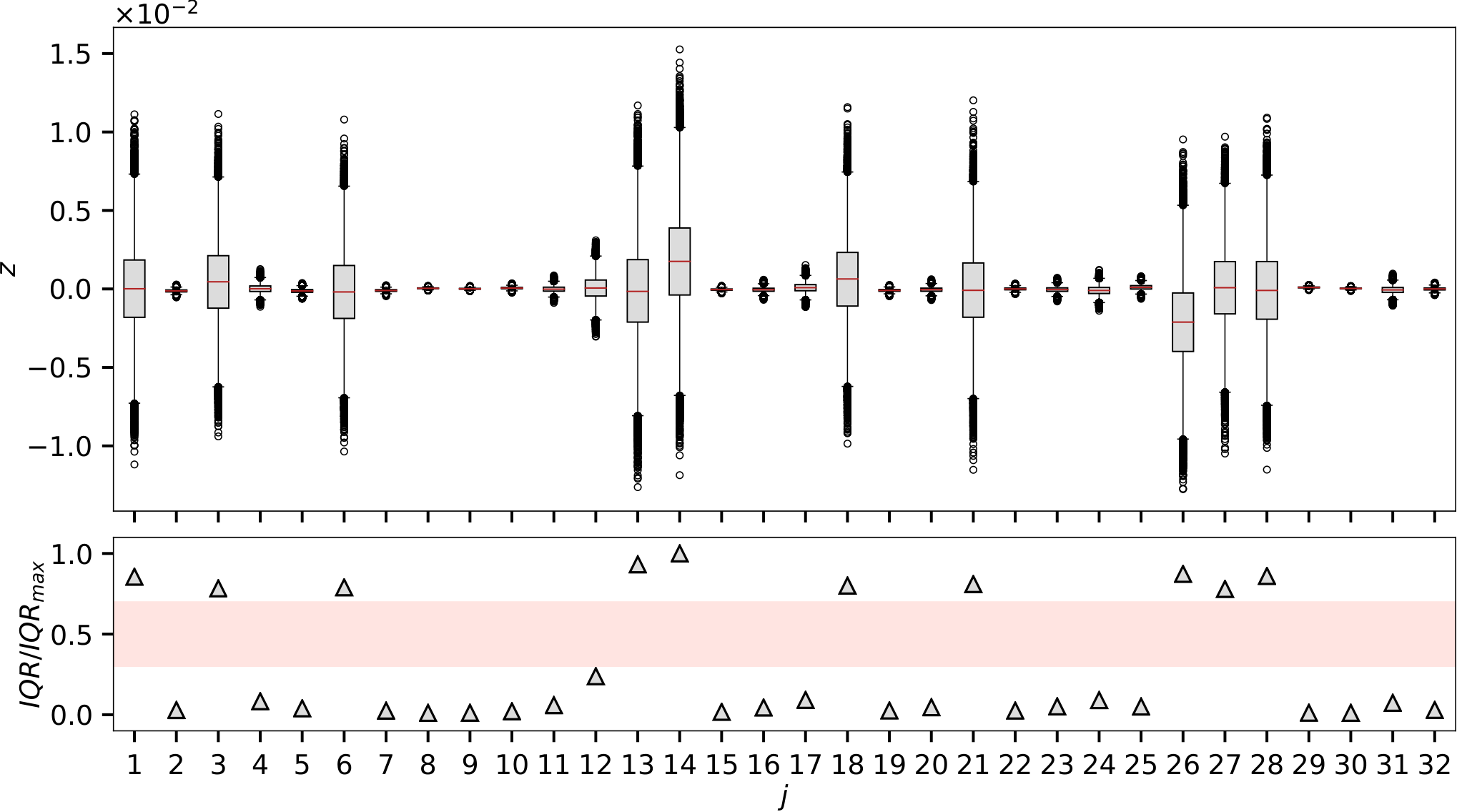
Figure 4 shows that of the latent dimensions, only are consistently active. This is consistent with, but slightly larger than, the known dimension of the inertial manifold for the K-S equation Yang and Radons 2012; Ding et al. 2016.
Figure 4: Active latent dimensions for the model with the lowest total loss (3) (). Top: Box plots of each dimension of the latent space generated by passing all snapshots through the autoencoder and extracting the latent space. Bottom: Normalized for each dimension showing a gap between the active and remaining non-active dimensions.
The interquartile range () can be used as an indicator of the variability of the latent dimensions. When normalized by the largest (the most active latent dimension) a very clear separation between “active” and “non-active” dimensions emerges as shown in the bottom of Figure 4. The largest of the remaining dimensions is of the most active dimension.
The trained autoencoder model also provides a way to develop a nonlinear basis for the learned manifold using the technique of activation maximization.
The idea behind this technique is to determine the input that maximizes the output of a specific node in the neural network. In the present work, we were interested in the inputs that would maximize each latent dimension. The input that maximized a given latent dimension was interpreted as a component of the basis of the low-dimensional manifold. The input that maximizes latent dimension is determined from,
(6)
where
(7)
and
(8)
is a regularization used to smooth the resulting field with the regularization parameter . The function evaluation corresponds to an evaluation of the encoder portion of the trained autoencoder with input . Note that is not a temporal snapshot of the dataset, but instead represents an arbitrary input to the autoencoder. Gradient ascent was used to solve (6),
(9)
The step size was set to and the regularization strength was set to . The maximization of each latent dimension was initialized from a random distribution in space where each point was drawn uniformly in . The result is a basis for the reduced manifold. Figures 5a and 5c show the components of the basis and their power spectra, respectively. The power spectra clearly show that the components of the discovered basis consist of a handful of distinct modes. In contrast to the active dimensions, Figures 5b and 5d show that the inputs that maximize the non-active dimensions are constants near zero.
(a)
(b)
(c)
(d)
Figure 5: (a) The nonlinear basis for the dimensional manifold found for the K-S equation with . (b) Examples of the non-active dimensions. (c) Power spectrum of the basis for the active dimensions. (d) Power spectrum of two non-active dimensions. Wavenumbers in the power spectra have been truncated to highlight the peaks in the power spectra. There are no peaks for .
Finally, we compute the optimal number of latent dimensions for and repeat the experiment ten times for each value of . Figure 6 depicts the scaling of the number of latent dimensions with , along with uncertainty bounds, and shows a nearly linear scaling, consistent with the scaling of the number of active modes Yang et al. 2009.
Figure 6: Scaling of the optimal number of latent dimensions with domain size for the K-S equation.
IV.2 KdV Equation
The latent space penalization enabled the discovery of a reduced basis for an equation that has an inertial manifold. In contrast to the K-S equation, the undamped KdV equation does not possess an inertial manifold and, moreover, the dynamics are truly infinite dimensional Ghidaglia 1988. The undamped KdV equation therefore provides a test for the method in which the optimal latent space penalization is expected to be zero. Before training the autoencoder, the input was normalized by its maximum value. Following the same procedure as for the K-S equation, the optimal latent space regularization was determined to be implying that the system does not possess an underlying finite-dimensional manifold. Figure 3 (c) presents a snapshot of a solution from the validation set and the corresponding prediction from the autoencoder at . The lack of a finite-dimensional manifold is further supported by Figure 7, in which the for each snapshot of the dataset is visualized for each dimension in the latent space. There is no separation of the latent space dimensions into “active” and “nonactive” components.
Figure 7: Active latent dimensions for the KdV equation at visualized with the normalized . The least active dimension is more than of the most active dimension indicating that all latent dimensions are required to reconstruct the solution.
IV.3 Damped KdV Equation
As a final test case, the damped KdV equation was studied over a range of damping coefficients, (see Table 1 in Appendix A). The damped KdV equation possesses an inertial manifold and it therefore provides a fertile test ground for understanding the behavior of the latent space as the damping coefficient is varied. For each damping coefficient, the autoencoder with latent space penalization was trained across a number of regularization parameters. The number of active dimensions for each damped KdV equation had to be determined. However, the minima in the MSE loss, vs. regularization parameter, , on the validation sets were shallow. Figure 8a presents a representative example for one particular model. Rather than extract a single minimum as was done in the K-S case, a different procedure was employed to provide a more robust result.
As before, the model with the minimum validation loss was extracted at each and used for the analysis. Instead of retaining a single model at the minimum of the curve, all models were retained in the shallow minimum. The latent dimensions for every snapshot of the dataset were computed for each of these models and the was again used to assess the activity of each latent dimension. The number of active dimensions was computed by counting the number of latent dimensions with above a certain threshold, , for each model. To guard against sensitivity in the choice of , a range of thresholds was tested between and . This process results in an array representing the number of active dimensions for each value of . The array contains the number of active dimensions for each model in the shallow minimum and each threshold value. The median number of dimensions over each model in the shallow minimum for each case and each threshold value was computed, which resulted in an array for each case that represents the number of active dimensions for each choice of threshold. As expected, the threshold value only shifts the number of active dimensions up and down, but the behavior of the number of active dimensions over for each threshold value remains the same. The final result is obtained by taking the median over the threshold values. Figure 8b shows the variation of active dimensions as the threshold is increased.
(a)
(b)
Figure 8: (a) Validation loss as a function of regularization parameter for the damped KdV equation with . The dashed line is presented as a reference to highlight the shallow minimum / plateau. (b) The number of active dimensions as a function of damping parameter for different thresholds. The mean and median show the overall scaling. The paper presents the median.
The number of active latent dimensions decreases nearly monotonically with increasing damping coefficient as shown in Figure 9.
Figure 9: Active latent space dimensions vs. damping parameter for the damped KdV equation.
V Conclusions
We introduced an autoencoder with latent space penalization applied to datasets generated from nonlinear partial differential equations in physics. The latent space penalization is used to restrict the dimensionality of the latent space to the minimal number of dimensions, thereby ensuring that the dynamics embodied in the dataset are captured by a low-dimensional manifold. In the case of the K-S equation, the optimal latent space dimension was consistent with the known dimensionality of the inertial manifold for bifurcation parameter . We then determined a nonlinear basis for this manifold, which could in principle be used in a reduced order model. The KdV equation does not posses an inertial manifold and has truly infinite dimensional dynamics. In this case, we found optimal results without any latent space penalization, which is consistent with the known properties of the KdV equation. Finally, when applying this technique to the damped KdV equation, which once again has an inertial manifold, we found the beginnings of power law scaling for the number of active dimensions for sufficiently large damping coefficient. This technique opens interesting directions for determining reduced order models.
Acknowledgements.
The authors thank Michael Jolly and Robert Moser for insightful discussions. The computations in this paper were run on the FASRC Cannon cluster supported by the FAS Division of Science Research Computing Group at Harvard University.
References
Schmid and Sesterhenn (2008)
P. Schmid and
J. Sesterhenn,
APS 61, MR
(2008).
Schmid (2010)
P. J. Schmid,
Journal of fluid mechanics 656,
5 (2010).
Benner et al. (2015)
P. Benner,
S. Gugercin, and
K. Willcox,
SIAM review 57,
483 (2015).
Swischuk et al. (2019)
R. Swischuk,
L. Mainini,
B. Peherstorfer,
and K. Willcox,
Computers & Fluids 179,
704 (2019).
Lagaris et al. (1998)
I. E. Lagaris,
A. Likas, and
D. I. Fotiadis,
IEEE transactions on neural networks
9, 987 (1998).
Raissi et al. (2017)
M. Raissi,
P. Perdikaris,
and G. E.
Karniadakis, arXiv preprint
arXiv:1711.10561 (2017).
Wu et al. (2018)
J.-L. Wu,
H. Xiao, and
E. Paterson,
Physical Review Fluids 3,
074602 (2018).
Raissi et al. (2019)
M. Raissi,
P. Perdikaris,
and G. E.
Karniadakis, Journal of Computational
Physics 378, 686
(2019).
Greydanus et al. (2019)
S. Greydanus,
M. Dzamba, and
J. Yosinski, in
Advances in Neural Information Processing Systems
(2019), pp. 15379–15389.
Brenner et al. (2019)
M. Brenner,
J. Eldredge, and
J. Freund,
Physical Review Fluids 4,
100501 (2019).
Qian et al. (2020)
E. Qian,
B. Kramer,
B. Peherstorfer,
and K. Willcox,
Physica D: Nonlinear Phenomena
406, 132401
(2020).
Mattheakis et al. (2020)
M. Mattheakis,
D. Sondak,
A. S. Dogra, and
P. Protopapas,
arXiv preprint arXiv:2001.11107 (2020).
Page et al. (2020)
J. Page,
M. P. Brenner,
and R. R.
Kerswell, arXiv preprint arXiv:2008.07515
(2020).
Gonzalez and Balajewicz (2018)
F. J. Gonzalez and
M. Balajewicz,
arXiv preprint arXiv:1808.01346 (2018).
Kuptsov and Kuptsova (2019)
P. V. Kuptsov and
A. V. Kuptsova, in
Saratov Fall Meeting 2018: Computations and Data
Analysis: from Nanoscale Tools to Brain Functions
(International Society for Optics and Photonics,
2019), vol. 11067, p.
110670N.
Champion et al. (2019)
K. Champion,
B. Lusch,
J. N. Kutz, and
S. L. Brunton,
Proceedings of the National Academy of Sciences
116, 22445
(2019).
Linot and Graham (2020)
A. J. Linot and
M. D. Graham,
Physical Review E 101,
062209 (2020).
Gilpin (2020)
W. Gilpin,
arXiv preprint arXiv:2002.05909 (2020).
Kuramoto and Tsuzuki (1976)
Y. Kuramoto and
T. Tsuzuki,
Progress of theoretical physics
55, 356 (1976).
Cohen et al. (1976)
B. I. Cohen,
J. Krommes,
W. Tang, and
M. Rosenbluth,
Nuclear fusion 16,
971 (1976).
Sivashinsky (1977)
G. Sivashinsky,
AcAau 4, 1177
(1977).
Sivashinsky and
Michelson (1980)
G. I. Sivashinsky
and
D. Michelson,
PThPh 63, 2112
(1980).
Nicolaenko et al. (1985)
B. Nicolaenko,
B. Scheurer, and
R. Temam,
Physica D: Nonlinear Phenomena
16, 155 (1985).
Foias et al. (1988)
C. Foias,
B. Nicolaenko,
G. Sell, and
R. Temam,
Journal de Mathématiques Pures et Appliquées
67, 197 (1988).
Conte and Musette (1989)
R. Conte and
M. Musette,
Journal of Physics A: Mathematical and General
22, 169 (1989).
Jolly et al. (1990)
M. S. Jolly,
I. Kevrekidis,
and E. S. Titi,
Physica D: Nonlinear Phenomena
44, 38 (1990).
Robinson (1994)
J. C. Robinson,
Physics Letters A 184,
190 (1994).
Jolly et al. (2000)
M. S. Jolly,
R. Rosa,
R. Temam,
et al., Advances in Differential Equations
5, 31 (2000).
Constantin et al. (2012)
P. Constantin,
C. Foias,
B. Nicolaenko,
and R. Temam,
Integral manifolds and inertial manifolds for
dissipative partial differential equations, vol. 70
(Springer Science & Business Media,
2012).
Ding et al. (2016)
X. Ding,
H. Chaté,
P. Cvitanović,
E. Siminos, and
K. Takeuchi,
Physical review letters 117,
024101 (2016).
Korteweg and De Vries (1895)
D. J. Korteweg and
G. De Vries,
The London, Edinburgh, and Dublin Philosophical Magazine
and Journal of Science 39, 422
(1895).
Kassam and Trefethen (2005)
A.-K. Kassam and
L. N. Trefethen,
SIAM Journal on Scientific Computing
26, 1214 (2005).
Rumelhart et al. (1985)
D. E. Rumelhart,
G. E. Hinton,
and R. J.
Williams, Tech. Rep.,
California Univ San Diego La Jolla Inst for Cognitive
Science (1985).
Baldi (2012)
P. Baldi, in
Proceedings of ICML workshop on unsupervised and
transfer learning (2012), pp. 37–49.
Milano and Koumoutsakos (2002)
M. Milano and
P. Koumoutsakos,
Journal of Computational Physics
182, 1 (2002).
Mikolov et al. (2012)
T. Mikolov et al.,
Presentation at Google, Mountain View, 2nd April
80, 26 (2012).
Kingma and Ba (2014)
D. P. Kingma and
J. Ba, arXiv
preprint arXiv:1412.6980 (2014).
Yang and Radons (2012)
H.-l. Yang and
G. Radons,
Physical review letters 108,
154101 (2012).
Yang et al. (2009)
H.-l. Yang,
K. A. Takeuchi,
F. Ginelli,
H. Chaté,
and G. Radons,
Physical review letters 102,
074102 (2009).
Appendix A Numerical Simulations
The one-dimensional Kuramoto-Sivashinsky (K-S) and Korteweg-de Vries (KdV) equations were solved using a pseudo-spectral Fourier discretization in space and an exponential fourth-order Runge-Kutta method Kassam and Trefethen 2005 in time. The spatial domain was discretized using points in physical space. The nonlinear terms were computed in physical space using the dealiasing rule. Table 1 presents the runs that were used to generate the figures in the paper.
Table 1: Details of the numerical simulations that were used to generate the datasets. The damping coefficient only applies to the damped KdV equation. represents the number of discrete points in the physical domain. The final integration time is and the constant time step is given by .
Case
Equation
Domain
1
K-S
—
2
K-S
—
3
K-S
—
4
K-S
—
5
K-S
—
6
K-S
—
7
K-S
—
8
K-S
—
9
KdV
10
KdV
11
KdV
12
KdV
13
KdV
14
KdV
15
KdV
16
KdV
17
KdV
18
KdV
19
KdV
20
KdV
21
KdV
22
KdV
Appendix B Autoencoder Architectures
Table 2: Parameters used for the trained autoencoders. The cases correspond to those in Table 1. The Start Index column represents the snapshot index from which the training and validation sets were taken. Data before this index was not used.