Emission of magnetar bursts and precursors of neutron star mergers

The typical energy budget of a magnetar burst ${\cal E}\mathrel{\hbox{\raise 2.15277pt\hbox{$<$}\hbox to0.0pt{\hss\lower 2.15277pt\hbox{$\sim$}}}}10^{41}\,$erg corresponds to a weak perturbation of the inner magnetosphere $\delta B_{\star}/B_{\star}\sim 10^{-3}-10^{-2}$. Such perturbations are expected from starquakes (Blaes et al. 1989; Thompson96; Bransgrove et al. 2020). It is less clear how they generate short X-ray bursts, as this requires quick dissipation of the initially ideal MHD perturbation, on a timescale $\sim 0.1\,$s.

A possible way for fast dissipation involves launching the perturbation along extended magnetic field lines, into the outer magnetosphere, where the relative wave amplitude $\delta B/B$ grows as $B^{-1/2}\propto R^{3/2}$. Then, the waves can reach $\delta B/B\sim 1$ at $R\sim(30-100)R_{\star}$ and dissipation can immediately occur through magnetic reconnection, as demonstrated by Yuan20. Energy dissipated in such events, ${\cal E}_{\rm diss}$, is a fraction of the outer magnetosphere energy,

where $\mu=B_{\star}R_{\star}^{3}=10^{33}B_{\star,15}R_{\star,6}^{3}$ is the magnetic dipole moment of the star. Magnetar bursts have energies consistent with ${\cal E}_{\rm diss}\mathrel{\hbox{\raise 2.15277pt\hbox{$>$}\hbox to0.0pt{\hss\lower 2.15277pt\hbox{$\sim$}}}}0.1{\cal E}_{\rm mag}$ at $R\sim(0.3-1)\times 10^{8}\,$cm.

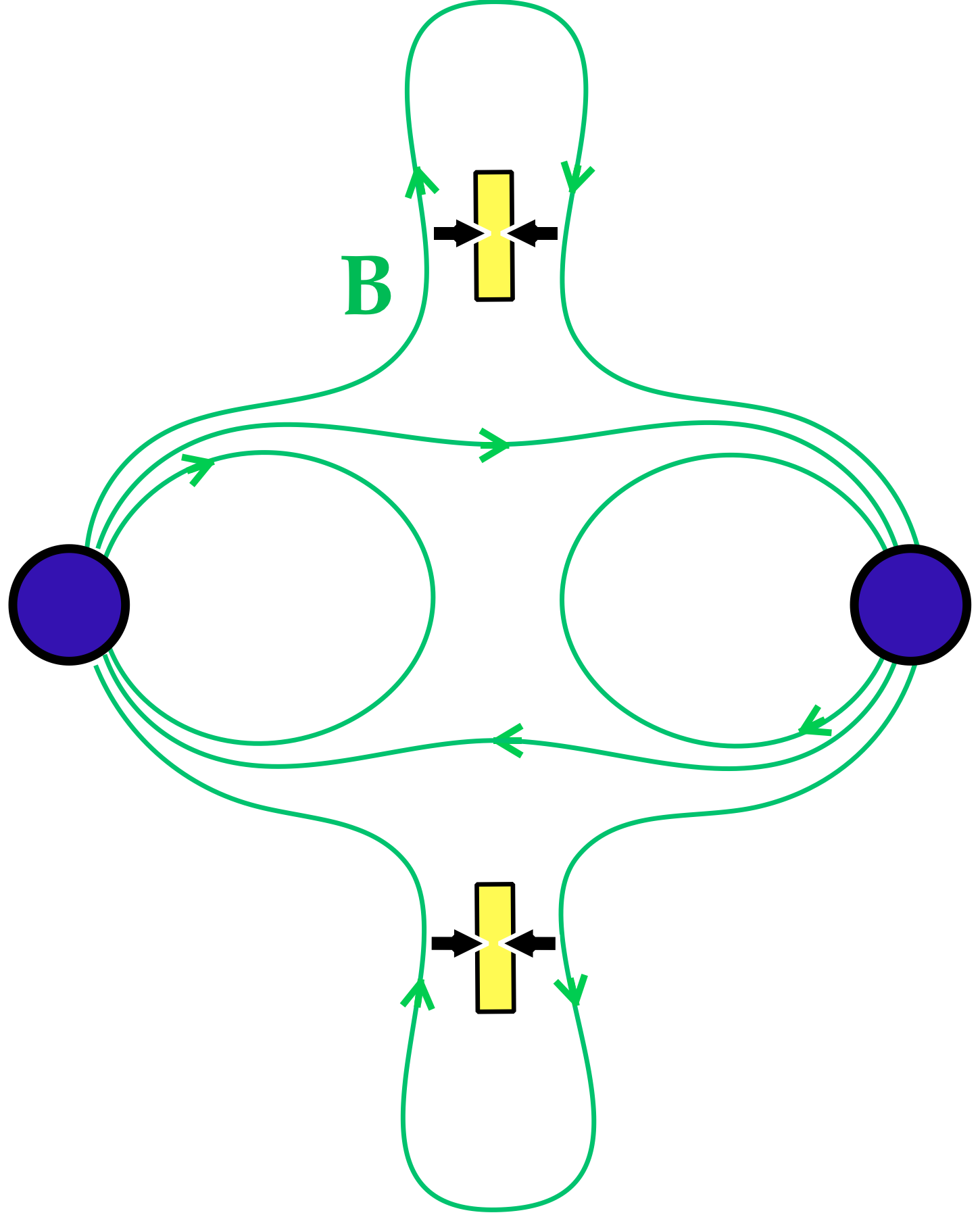
Similar magnetic dissipation events are expected during magnetospheric interaction in a binary neutron star (Most20). In this case, the field lines connecting the two stars can be continually twisted by their asynchronous rotation, which pumps $\delta B/B\mathrel{\hbox{\raise 2.15277pt\hbox{$>$}\hbox to0.0pt{\hss\lower 2.15277pt\hbox{$\sim$}}}}1$ and drives quasi-periodic magnetic flares. Figure 1 shows the flaring magnetosphere of a binary system in the simple case of (anti) parallel magnetic dipole moments of the stars. For comparison, Figure 1 also illustrates a magnetic flare in an isolated magnetar.

In both cases, the flare develops through sudden unstable inflation of the magnetosphere outside some radius $R$. It happens where the magnetic twist $\delta B$ exceeds the original field $B$ by a numerical factor $\mathrel{\hbox{\raise 2.15277pt\hbox{$>$}\hbox to0.0pt{\hss\lower 2.15277pt\hbox{$\sim$}}}}1$, which depends on the geometry and the rate of twisting (Parfrey13). This inflation creates a configuration with two opposite magnetic fluxes separated by a current sheet. The sheet thickness collapses under the magnetic pressure, and reconnection is triggered by the tearing instability breaking the current sheet into threads.

Relativistic magnetic reconnection occurs with speed $v_{\rm rec}\approx 0.1c$ (Kagan et al. 2015). Therefore, the magnetic flare is expected to occur on the timescale

As a result, the inflated magnetic field lines snap back to their original configuration, losing the twist and ejecting plasmoids from the magnetosphere. The characteristic size of the reconnection region $S$ (the half-length of the yellow regions in Figure 1) is a fraction of radius $R$. Its half-thickness is $H\sim(v_{\rm rec}/c)S\sim 0.1S$.

Part of the magnetic energy flux flowing through the reconnection region $v_{\rm rec}B^{2}/8\pi$ gets dissipated. The maximum dissipated fraction of $0.5$ is approached if the guide field $B_{\rm gd}$ (the magnetic field component along the electric current) is small, $B_{\rm gd}\ll\delta B$ (e.g. Sironi20). The resulting dissipation rate per unit volume (inside the layer of thickness $2H=2Sv_{\rm rec}/c$) may be written as

where $\zeta<0.5$.

Both analytical theory (Uzdensky10) and first-principle kinetic simulations (e.g. Sironi14) show that the current sheet breaks up into a chain of plasmoids with a broad (self-similar) distribution of sizes, from the microscopic Larmor radius to the macroscopic size $\sim H$. The plasmoids are accelerated by magnetic stresses and ejected along the reconnection layer, allowing reconnection to proceed with speed $v_{\rm rec}\approx 0.1c$.

Reconnection in magnetars and neutron star binaries operates in a highly radiative regime — essentially all dissipated energy immediately converts to radiation. The heat capacity of the plasma particles is negligible compared with that of photons; particles carry $\sim 10^{-5}$ of the dissipated energy in a typical magnetic flare, as shown below. Under such conditions, reconnection directly heats photons rather than the plasma. Photons receive energy by scattering off the moving plasmoids, and magnetic energy is dissipated by photon viscosity, which damps the plasmoid motions driven by magnetic stresses (Beloborodov 2017a). Note also that the fluid bulk motions in radiative reconnection exceed the particle thermal motions measured in the fluid rest frame.

Radiation receives energy as follows:
(1) Photons gain energy in scattering. As long as electron recoil is neglected (Thomson scattering), photons in the reconnection layer continue to drift upward in energy $E$ with a rate proportional to $E$, similar to Fermi acceleration. Their energy gain per Thomson scattering $(\overline{\Delta E}/E)_{\rm T}$ depends on the state of the plasma and defines the effective Comtponization temperature

Compton recoil in scattering is negligible for photons with $E\ll T_{\rm eff}$, and the reconnection layer upscatters such photons just like a static Maxwellian electron gas with temperature $T_{\rm eff}$ would do. Electron recoil in scattering becomes significant at $E\sim kT_{\rm eff}$. It steals photon energy $(\overline{\Delta E}/E)_{\rm recoil}=-E/m_{e}c^{2}$ and suppresses photon population at $E\gg kT_{\rm eff}$. The small population of energetic photons with $E\gg kT_{\rm eff}$ is still crucial, because it controls $e^{\pm}$ pair creation.
(2) The $e^{\pm}$ plasma produces new photons with energies $E_{0}\ll kT_{\rm eff}$. The rate of photon production $\dot{n}_{\rm ph}$ is given in Section 3 below. This rate is controlled by the plasma density and its true temperature $T$ measured in the fluid frame, rather than by $T_{\rm eff}$.

Photon production gives more photons to share the dissipated power, lowering energy per photon. When emission proceeds in a quasi-steady regime, the average energy of escaping photons $\overline{E}_{\rm esc}$ satisfies the relation

which assumes $\overline{E}_{\rm esc}\gg E_{0}$. Ratio $\overline{E}_{\rm esc}/kT_{\rm eff}$ is related to the spectral slope of escaping radiation, which extends from $E_{0}$ to $kT_{\rm eff}$.

Creation of $e^{\pm}$ pairs endows the reconnection layer with a signifcant Thomson optical depth, up to $\tau_{\rm T}\sim 10$ in the models calculated below. Then, very large plasmoids can trap and advect radiation while smaller plasmoids move through radiation, experiencing Compton drag. This means that photon viscosity operates on scales smaller than the size of the layer. This is similar to photon viscosity in optically thick turbulence cascades (Zrake19).

Photon viscosity (Compton drag) implies that current density $J$ in a plasma with density $n_{\pm}$ is accompanied by energy losses per particle $\dot{E}_{e}\sim c\sigma_{\rm T}U(J/en_{\pm}c)^{2}$, where $U$ is the radiation energy density. Losses per unit volume, $n_{\pm}\dot{E}_{e}$, may be written as $J^{2}/\tilde{\sigma}$ with effective conductivity $\tilde{\sigma}$. This gives $\tilde{\sigma}\sim ce^{2}n_{\pm}/\sigma_{\rm T}U$ and the magnetic diffusivity

A classical Sweet-Parker resistive reconnection layer would have relative thickness $\delta_{\rm SP}/S\sim(\eta/cS)^{1/2}$, and its tearing instability would create structures as thin as $\delta_{\eta}\sim 100\eta/c$ (Uzdensky10). For typical parameters of our burst model $\delta_{\eta}\ll c/\omega_{p}$, where $\omega_{p}=(4\pi e^{2}n_{\pm}/m_{e})^{1/2}$ is the plasma frequency. Therefore, the small-scale reconnection does not obey the resistive MHD. Instead, it proceeds in the collisionless regime, with speed $\sim 0.1c$, as confirmed by kinetic simulations with Compton drag (Sironi20). Note also that the characteristic electron free path due to photon viscosity may be written as $\lambda\sim S/\ell$, where $\ell\sim 10^{5}-10^{7}$ is the radiation compactness parameter (Equation (9) below). Our burst models have

This is different from reconnection in ultrastrong fields $B>10^{13}\,$G, which could proceed in the resistive MHD regime (Uzdensky11).

Despite the strong collisionless dynamics of the reconnection layer on microscopic scales, most of magnetic dissipation occurs on scales $\gg\lambda$, through radiation drag on the moving macroscopic plasmoids. Energy is extracted from the field due to work of the ideal MHD force $\boldsymbol{J}\times{\,\mathbf{B}}/c$ rather than ohmic dissipation of currents.

The dissipation process described above is similar to pulling bodies (plasmoids) by strings (magnetic field lines) against a viscous background (radiation). Radiative kinetic plasma simulations suggest that this process accounts for $\sim 80$% of total dissipation (Sironi20). The remaining fraction goes into nearly impulsive acceleration (“injection”) of nonthermal particles. The injection occurs near X-points in the reconnection layer and operates on the timescale as short as

where $\omega_{B}=eB/m_{e}c$ is the gyro-frequency. The maximum accelerating electric field $E\sim(v_{\rm rec}/c)B\sim 0.1B$ is capable of pushing particles to Lorentz factors $\gamma\sim\sigma_{0}=B^{2}/4\pi m_{e}c^{2}n_{\pm}$ on the timescale $t_{\rm acc}$. However, for the typical parameters of our burst model, radiative losses stop the acceleration at $\gamma_{\rm cr}\sim(S/\ell r_{e})^{1/4}\sim 10^{3}<\sigma_{0}$. Thus, X-point injection is drag-limited, in contrast to previously discussed magnetic flares near accreting black holes, where $\gamma_{\rm cr}>\sigma_{0}$ (Beloborodov 2017a).

The vast majority of injection events give small $\gamma\sim 1$ (see Figure 8 in Sironi20); they occur via particle “pick up” by outflows from X-points. The simulations with magnetization $\sigma_{0}=10$ show that a few percent of the dissipated power is spent to inject highly relativistic particles. Note however that magnetic flares around neutron stars have much greater $\sigma_{0}$, and radiative kinetic simulations with higher magnetizations are needed to clarify the scaling of injection with $\sigma_{0}$. Below we use a simple parametrization of high-energy particle injection to study its effect on the burst emission.

Alfvén waves that do not reach $\delta B/B>1$ keep bouncing in the closed magnetosphere for some time and eventually dissipate, without triggering large-scale magnetic reconnection. Their dissipation may occur via a turbulence cascade developing due to nonlinear effects (Thompson98; Li et al. 2019). Furthermore, dissipation may result from the shearing of Alfvén wave packets as they propagate along the curved magnetic field lines, which enhances the electric current density (Bransgrove et al. 2020; Chen et al. 2020).

The dissipation process is not well understood for the waves with $\delta B<B$. If it does occur quickly, its radiative effect will be similar to that of magnetic reconnection. The radiative calculations below can be applied to any type of fast dissipation in the outer magnetosphere.

The power $L$ dissipated in the magnetic flare immediately converts to radiation, i.e. $L$ is also the radiation production rate. The corresponding dimensionless compactness parameter is defined by

where $2S$ is the size of the dissipation region (Figure 2). The flare is fed by magnetic energy in the dissipation region of volume $V\sim 2S\times 2S\times 2H$.¹¹ 1 The dissipation region may be composed of $N$ regions of volume $2S\times 2S\times 2H$, giving the total observed luminosity $L_{\rm tot}=NL$. For example, reconnection in an axisymmetric magnetosphere forms a dissipation region $2\pi R\times 2S\times 2H$; then $N\sim 10$. The volume-average energy release rate is

It may also be expressed as in Equation (3), which gives the relation

where

The only dimensional parameter of the problem is $S\sim 10^{7}\,$cm; it determines $B$ for given $\ell$ and $\zeta$.

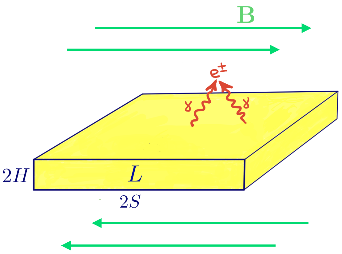
The formulation of the burst problem is simple:²² 2 This formulation of the burst problem is applicable to both magnetic reconnection and dissipation of Alfvén wave turbulence. there is an initially empty region of volume $V$ where magnetic energy is released with a given power $L$. The dissipation event lasts for $t_{\rm diss}\gg S/c$ (Equation 2). The magnetic field $B$ in the region and the released power $L$ are related by Equation (11). The question is what radiation is emitted by this dissipation event.

In a real magnetosphere, the “empty” region contains some seed plasma and radiation. Magnetic dissipation starts with accelerating seed particles, producing inverse Compton emission and igniting pair creation. Regardless of the initial state, the high compactness parameter $\ell$ guarantees that the region becomes filled with dense radiation and $e^{\pm}$ plasma (Cavallo & Rees 1978).

The $e^{\pm}$ density $n_{\pm}$ in the dissipation region is not known in advance and needs to be calculated self-consistently. It will determine the characteristic optical depth

A simple estimate shows that the self-consistent $n_{\pm}$ is much lower than the photon number density $n_{\rm ph}=U/\bar{E}$, where $\bar{E}$ is the average photon energy inside the source and $U$ is the radiation density. When the burst is emitted via quasi-steady diffusion of radiation, one can estimate $L\sim VU/t_{\rm diff}$, where $t_{\rm diff}\sim\tau_{\rm T}H/c$. This gives the relation $L\sim 8S^{2}\bar{E}n_{\rm ph}c/\sigma_{\rm T}Hn_{\pm}$, and so,

This also gives an estimate for the magnetization parameter of the dissipation region,

We will use a uniform statistical description of the plasma motions in the dissipation region. Photons have macroscopic free paths $\sim H/\tau_{\rm T}$ and randomly sample the four-velocity $u=\gamma\beta$ of the scattering particles. In our simulations, $u$ in each scattering event is drawn from a single global particle distribution $f_{e}(u)$. This approximation is much simpler than a full kinetic plasma simulation of magnetic reconnection coupled to radiative transfer, a challenge for future work.

The main parameter of $f_{e}(u)$ is the integral

It determines the rate of energy gain of radiation from scattering $\dot{U}_{\rm C}$ (see the definition of $T_{\rm eff}$ in Equation 4). Note that $\Theta_{\rm eff}$ is not known in advance and can evolve in the self-consistent radiative model of the burst. For any given instantaneous state of radiation, $T_{\rm eff}(t,x,y,z)$ must satisfy the local energy balance,

It states that the plasma immediately passes the dissipated energy to radiation, as the plasma heat capacity is negligible. The energy exchange rate $\dot{U}_{\rm C}(T_{\rm eff})$ depends on both the spectrum of radiation and the shape of $e^{\pm}$ distribution, $f_{e}(u)$. In our Monte-Carlo simulations below, $\dot{U}_{\rm C}(T_{\rm eff})$ is calculated numerically using the exact Klein-Nishina cross section for Compton scattering.

A simple analytical estimate for $\dot{U}_{\rm C}(T_{\rm eff})$ is obtained using Thomson approximation and assuming isotropic $e^{\pm}$ motions with $\Theta_{\rm eff}\ll 1$:

Here $U_{\epsilon}$ is the spectral energy density of radiation, $U=\int U_{\epsilon}\,d\epsilon$ is the total energy density, and $\epsilon=E/m_{e}c^{2}$. In a quasi-steady state, $U\sim\dot{U}_{\rm diss}t_{\rm diff}$ where $t_{\rm diff}\approx\tau_{\rm T}H/c$ is the diffusion time of radiation out of the heating region. Then the energy balance condition (17) simplifies to

The parameter $\Theta_{\rm eff}=\langle u^{2}/3\rangle$ can be determined for any given distribution function $f_{e}(u)$, which may have different shapes. In a standard model of thermal Comptonization, $f_{e}(u)$ would be Maxwellian,

where $\Theta_{\rm eff}$ is the only parameter. A realistic reconnection region is not quite Maxwellian: $f_{e}(u)$ has a sub-relativistic peak formed by plasmoid motions and a high-energy tail formed by impulsive particle acceleration near X-points. The tail steeply declines at $u\gg 1$. A simple example of a non-Maxwellian distribution is

It replaces the Maxwellian exponential cutoff with a power-law decline at $u\gg u_{0}$. The distribution function in Equation (21) has two parameters $u_{0}$ and $\alpha$. $\Theta_{\rm eff}(u_{0},\alpha)$ can be calculated from Equation (16), and a good approximation is given by

The power received and radiated by the high-energy tail at $u\gg u_{0}$ is proportional to $\int_{u}^{\infty}{u^{\prime}}^{2}f_{e}(u^{\prime})\,du^{\prime}\propto u^{-\alpha+3}$. In particular, the fraction of the dissipated power received by particles with $u>1$ is approximately given by

In magnetic flares, the power deposited into relativistic particles $u\gg 1$ is likely a small fraction of the total released power $\dot{U}_{\rm diss}$. This corresponds to $f_{e}(u)$ with a steep high-energy tail, $\alpha>5$. A strong nonthermal tail, $\alpha=5$, gives $\dot{U}_{1}/\dot{U}_{\rm diss}\approx 2\Theta_{\rm eff}$, which varies around 5% in the sample models calculated below.

The effect of the nonthermal high-energy tail in $f_{e}(u)$ will be illustrated below by calculating the burst spectra for the two choices of $f_{e}(u)$, Equations (20) and (21). In both Maxwellian and nonthermal plasma models, $f_{e}(u)$ has a single-peak shape: it grows as $f_{e}(u)\propto u^{2}$ at small $u^{2}<\Theta_{\rm eff}$ and falls off at high $u$. Therefore, the production of Comptonized radiation declines at $E\gg kT_{\rm eff}$. The weak high-energy part of the photon spectrum is important, because it controls the rate of $e^{\pm}$ creation in photon-photon collisions $\dot{n}_{\gamma\gamma}$ (see Section III.5 below). However, the feedback of $\dot{n}_{\gamma\gamma}$ on $T_{\rm eff}$ turns out modest, leading to $kT_{\rm eff}=10-40\,$keV for the entire range of relevant parameters (Section III.4).

The single global distribution $f_{e}(u)$ is convenient in the calculations of Comptonization. However, for the analysis of photon production, it is more convenient to view the plasma as the sum of two parts: thermal particles (which have a Maxwellian distribution in the plasma rest frame) and nonthermal particles injected near X-points.

The true plasma temperature $T$ (which enters the photon production rates given below) differs from $T_{\rm eff}$. It is defined in the plasma rest frame and locked to the Compton temperature,

This equality is enforced on the Compton timescale $t_{\rm C}$, which is much shorter than the light crossing time $S/c$,

The value of Compton temperature is found from

where $\dot{U}_{\rm C}(T)$ is calculated for a Maxwellian plasma (in its rest frame). A simple estimate for $\Theta_{\rm C}\equiv kT_{\rm C}/m_{e}c^{2}$ is obtained in the Thomson approximation and given in Equation (18). An accurate calculation of $T_{\rm C}$ would use the radiation spectrum $U_{\epsilon}$ Doppler boosted to the plasma rest frame. However, only a small fraction of the reconnection region (small plasmoids) has highly relativistic bulk speeds, and the thermal photon production is dominated by large plasmoids with mildly relativistic motions. Therefore, we will neglect the Doppler boost and find $T_{\rm C}$ from condition (26) in the fixed lab frame; this gives $\sim 10\%$ accuracy of $T$, leading to a similar accuracy of $\dot{n}_{\rm ph}$.

In general, thermal plasma in compact X-ray sources produces photons through three main processes: bremsstrahlung, double Compton scattering, and cyclo-synchrotron emission. These processes have been well studied, in particular in the context of accreting black holes and GRB explosions (Svensson84; Wardzinski00; Beloborodov 2013; Vurm13; Thompson14). The cyclo-synchrotron mechanism dominates in the magnetic flares of interest here. In addition, some photons may be produced by synchrotron emission from high-energy particles. The photon production mechanisms are summarized below.

In general, the boundary $\epsilon_{0}$ between the Rayleigh-Jeans and the Comptonization part of the photon spectrum determines $n_{\rm RJ}=\epsilon_{0}^{2}\Theta/2\pi^{2}\lambda\hbox to0.0pt{\hss--}^{3}$ and implies photon supply with rate $\dot{n}_{\rm ph}\approx 3n_{\rm RJ}\Theta_{\rm eff}c\sigma_{\rm T}n_{\pm}$. This gives the relation

It is valid regardless of the photon emission mechanism. In a quasi-steady state, the condition $\dot{n}_{\rm ph}\approx\dot{U}_{\rm diss}/\overline{E}_{\rm esc}$ gives

This “photon balance” condition imposes a relation between $n_{\pm}$ and $\Theta_{\rm eff}$.

Photon production in the neutron star bursts is dominated by cyclo-synchrotron emission, which has a special feature: $\epsilon_{0}^{2}$ is proportional to the magnetic energy density $U_{B}$. Since $\dot{U}_{\rm diss}=\zeta U_{B}c/S$ also scales with $U_{B}$, the parameter $\ell_{B}$ practically drops out from Equation (40), and one finds

Note that $\Theta$, $\Theta_{\rm eff}$, and $\overline{\epsilon}_{\rm esc}$ are all comparable. The detailed simulations presented below show that $\Theta$ is below $\Theta_{\rm eff}$, and $\overline{\epsilon}_{\rm esc}$ is above, so that $\Theta\Theta_{\rm eff}\overline{\epsilon}_{\rm esc}\sim\Theta_{\rm eff}^{3}$. Then, Equation (41) yields

where we substituted $\zeta H/S\approx 0.1\ell/\ell_{B}$ (Equation 11).

The evolution of $e^{\pm}$ density $n_{\pm}$ obeys the equation

Here $\dot{n}_{\rm ann}$ is the annihilation rate, written in the limit of $\Theta\ll 1$ (relativistic corrections to $\dot{n}_{\rm ann}$ are negligible at temperatures of interest $\Theta\mathrel{\hbox{\raise 2.15277pt\hbox{$<$}\hbox to0.0pt{\hss\lower 2.15277pt\hbox{$\sim$}}}}0.1$, see Equation (68) in Svensson82). Pairs are created with rate $\dot{n}_{\gamma\gamma}$ in collisions of photons with energies above $m_{e}c^{2}$, which receive a small fraction of the dissipated power.

The rate $\dot{n}_{\gamma\gamma}$ depends on the radiation spectrum formed by Comptonization. Radiation Comptonized by a Maxwellian distribution with temperature $T_{\rm eff}$ at high energies approaches a Wien spectrum,

with the effective $U_{\rm W}\sim(0.1-0.3)U$ depending on the overall shape of the Comptonized spectrum with the total density $U$. Pair creation in the Wien tail is given by (Svensson84)

When annihilation balance is established, $\dot{n}_{\gamma\gamma}\approx\dot{n}_{\rm ann}$, the $e^{\pm}$ density becomes

Then the relation $n_{\pm}m_{e}c^{2}/U\sim 8S/H\ell$ (Equation 14) gives

This requires $\Theta_{\rm eff}\approx 0.05-0.1$ in the entire relevant range of compactness parameter $\ell$, and implies that $\Theta_{\rm eff}$ very slowly decreases with $\ell$. The rough estimate of the numerical coefficient in Equation (47) is sufficient, because its variation weakly affects the solution for $\Theta_{\rm eff}$.

Comptonization by a nonthermal $e^{\pm}$ distribution $f_{e}(u)$ (Equation 21) produces a radiation spectrum with a power-law (rather than exponential) tail at $E\gg kT_{\rm eff}$. This leads to more efficient pair creation, so that the same $\tau_{\rm T}$ can be achieved at a lower $T_{\rm eff}$.

One can now check how quickly the injected photons with $E_{0}\ll kT_{\rm eff}$ get upscattered to energy $E\sim 3kT_{\rm eff}$ (where losses to Compton recoil become dominant). Photons gain energy $\Delta E/E=4\Theta_{\rm eff}$ per scattering and reach the peak after $N_{\rm W}\approx(4\Theta_{\rm eff})^{-1}\ln(3kT_{\rm eff}/E_{0})$ scatterings. This takes time $t_{\rm W}=N_{\rm W}/c\sigma_{\rm T}n_{\pm}$, and so

The regime of saturated Comptonization occurs if $t_{\rm W}$ is much shorter than the timescale for photon escape from the dissipation region, $t_{\rm esc}$. The photons can escape by diffusing across the reconnection layer on the timescale $t_{\rm diff}\approx\tau_{\rm T}H/c$, and

As long as $t_{\rm diff}$ represents the characteristic residence time of photons in the dissipation region, the ratio $t_{\rm diff}/t_{\rm W}$ controls the overall shape of the escaping radiation spectrum (Illarionov & Syunyaev 1972). The limit of $t_{\rm diff}/t_{\rm W}\rightarrow\infty$ gives the Wien spectrum $dn_{\rm ph}/d\ln E=0.5\,(E/kT)^{3}\exp(-E/kT)$, which peaks at $E=3kT$. A small $t_{\rm diff}/t_{\rm W}\mathrel{\hbox{\raise 2.15277pt\hbox{$<$}\hbox to0.0pt{\hss\lower 2.15277pt\hbox{$\sim$}}}}1$ gives a soft spectrum with an exponential cutoff at $E\sim kT_{\rm eff}$.

Using the photon balance condition (Equation 42), we find

Since $\Theta_{\rm eff}$ is self-regulated, so that it varies in a narrow range, Equation (50) gives $0.3\mathrel{\hbox{\raise 2.15277pt\hbox{$<$}\hbox to0.0pt{\hss\lower 2.15277pt\hbox{$\sim$}}}}t_{\rm diff}/t_{\rm W}\mathrel{\hbox{\raise 2.15277pt\hbox{$<$}\hbox to0.0pt{\hss\lower 2.15277pt\hbox{$\sim$}}}}3$ in a broad region of the parameter space. The variation of $t_{\rm W}/t_{\rm diff}$ between different models presented below causes (moderate) variations in the spectral slopes. In all cases, Comptonization occurs in the unsaturated regime.

In a reconnection layer, the moving magnetic field lines advect the $e^{\pm}$-photon fluid (coupled by scattering). If $\tau_{\rm T}$ exceeds $c/v_{\rm rec}$, radiation diffusion becomes slower than advection. Then a large part of the generated radiation can be advected sideways along the reconnection layer and ejected together with the magnetic plasmoids on the timescale $\sim S/c$. This timescale is shorter than $t_{\rm diff}$ when $\tau_{\rm T}>c/v_{\rm rec}$.

In general, the photon residence time in the quasi-steady dissipation region is $t_{\rm esc}\sim t_{\rm diff}$ in the diffusion-dominated regime, and $t_{\rm esc}\sim S/c$ in the advection-dominated regime:

The high $\tau_{\rm T}$ in the advection-dominated regime must be accompanied by a reduced $\Theta_{\rm eff}$, according to the photon balance condition (Equation 42). This situation occurs if the dissipation generates a nonthermal $e^{\pm}$ distribution with a significant high-energy tail. Compared with a Maxwellian plasma, the nonthermal $e^{\pm}$ are more efficient in Comptonizing photons to $E>m_{e}c^{2}$, enhancing $e^{\pm}$ creation, so that a high $\tau_{\rm T}>10$ can be achieved even when $\Theta_{\rm eff}$ is below 0.05 (a numerical example will be calculated in Section 4).

In the advection dominated regime, the ratio $t_{\rm esc}/t_{\rm W}$, which controls the slope of the Comptonized spectrum, becomes

References

- Beloborodov (1999) Beloborodov, A. M. 1999, MNRAS, 305, 181, doi: 10.1046/j.1365-8711.1999.02384.x
- Beloborodov (2013) —. 2013, ApJ, 764, 157, doi: 10.1088/0004-637X/764/2/157
- Beloborodov (2017a) —. 2017a, ApJ, 850, 141, doi: 10.3847/1538-4357/aa8f4f
- Beloborodov (2017b) —. 2017b, ApJ, 843, L26, doi: 10.3847/2041-8213/aa78f3
- Beloborodov (2020) —. 2020, ApJ, 896, 142, doi: 10.3847/1538-4357/ab83eb
- Blaes et al. (1989) Blaes, O., Blandford, R., Goldreich, P., & Madau, P. 1989, ApJ, 343, 839, doi: 10.1086/167754
- Bochenek et al. (2020) Bochenek, C. D., Ravi, V., Belov, K. V., et al. 2020, Nature, 587, 59, doi: 10.1038/s41586-020-2872-x
- Bransgrove et al. (2020) Bransgrove, A., Beloborodov, A. M., & Levin, Y. 2020, ApJ, 897, 173, doi: 10.3847/1538-4357/ab93b7
- Cavallo & Rees (1978) Cavallo, G., & Rees, M. J. 1978, MNRAS, 183, 359, doi: 10.1093/mnras/183.3.359
- Chen et al. (2020) Chen, A. Y., Yuan, Y., Beloborodov, A. M., & Li, X. 2020, arXiv e-prints, arXiv:2010.15619. https://arxiv.org/abs/2010.15619
- Illarionov & Syunyaev (1972) Illarionov, A. F., & Syunyaev, R. A. 1972, Soviet Ast., 16, 45
- Kagan et al. (2015) Kagan, D., Sironi, L., Cerutti, B., & Giannios, D. 2015, Space Sci. Rev., 191, 545, doi: 10.1007/s11214-014-0132-9
- Kaspi & Beloborodov (2017) Kaspi, V. M., & Beloborodov, A. M. 2017, ARA&A, 55, 261, doi: 10.1146/annurev-astro-081915-023329
- Li et al. (2020) Li, C. K., Lin, L., Xiong, S. L., et al. 2020, arXiv e-prints, arXiv:2005.11071. https://arxiv.org/abs/2005.11071
- Li et al. (2019) Li, X., Zrake, J., & Beloborodov, A. M. 2019, ApJ, 881, 13, doi: 10.3847/1538-4357/ab2a03