Geometrically-induced localization of flexural waves on thin warped physical membranes
Abstract
We consider the propagation of flexural waves across a nearly flat, thin membrane, whose stress-free state is curved. The stress-free configuration is specified by a quenched height field, whose Fourier components are drawn from a Gaussian distribution with power law variance. Gaussian curvature couples the in-plane stretching to out-of-plane bending. Integrating out the faster stretching modes yields a wave equation for undulations in the presence of an effective random potential, determined purely by geometry. We show that at long times/lengths, the undulation intensity obeys a diffusion equation. The diffusion coefficient is found to be frequency dependent and sensitive to the quenched height field distribution. Finally, we consider the effect of coherent backscattering corrections, yielding a weak localization correction that decreases the diffusion coefficient proportional to the logarithm of the system size, and induces a localization transition at large amplitude of the quenched height field. The localization transition is confirmed via a self-consistent extension to the strong disorder regime.
I Introduction
Thin, elastic shells, whose lateral size is much larger than their thickness, arise in a diverse array of contexts and across systems spanning several orders of magnitude in length Kearey et al. 2009; Wang and Hu 2005; Bower et al. 1999. Though the initial theory was formulated more than a century ago, shells that retain curvature in the stress-free state exhibit complex solutions due to geometrically induced nonlinearity, which has continued to inspire research Vaziri and Mahadevan 2008; Lazarus et al. 2012; Bende et al. 2015. The mechanical properties of shells with curved stress-free states is vital to the functionality of a number of biological applications, including red blood cells Waugh and Evans 1979; Park et al. 2010; Park et al. 2011, viral capsids Lidmar et al. 2003; Ivanovska et al. 2004; Kuriabova and Levine 2008; Michel et al. 2006; Klug et al. 2006, and plant morphogenesis Dervaux and Amar 2008. Though these latter examples lack well defined elastic continua, they have nevertheless been successfully studied using thin shell theory.
The mechanics of thin shells are determined by geometry, and shells of different curvature in the stress-free state can exhibit wildly different characteristics Radzihovsky and Nelson 1991; Morse and Lubensky 1992; Radzihovsky and Le Doussal 1992; Le Doussal and Radzihovsky 1993. Due to Gauss’ theorema egregium, Gaussian curvature couples the typically soft bending undulations to the much stiffer stretching deformations. As a result, areas of positive Gauss curvature suppress bending undulations Vaziri and Mahadevan 2008, which can lead to spatially heterogenous pockets of large undulations separated by boundary curves of zero normal curvature, as has been observed in the fluctuations of red blood cells Evans et al. 2017. As undulations typically represent the softest elastic modes, these can have serious consequences on the ability for shells to equilibrate, which has applications for the stability of cell membranes with actively driven pumps.
An examination of undulatory waves in the geometric optics limits shows that Gauss curvature scatters undulatory waves, and can even lead to total internal reflection at boundaries where the sign changes Evans and Levine 2013. This suggests that for thin shells with random stress-free curvature, energy transport could be severely slowed, if not localized, purely as a consequence of geometry.
In this manuscript, we present an analysis of the propagation of undulatory waves through randomly curved thin shells that, in contrast to the large literature of wave propagation in random media Ishimaru 2017, is driven entirely by geometry. Wave propagation in random media has been extensively studied Akkermans and Montambaux 2007; Rammer 2018; van Rossum and Nieuwenhuizen 1999; Sheng 2006; Chakravarty and Schmid 1986 across a broad array of subjects Campillo and Paul 2003; Korn 1993; Bayer and Niederdränk 1993, which we use as a guide.
The outline of this paper is as follows. First, a general consequence of random scattering is to shift energy propagation from ballistic to diffusive, which we quantitatively compute in the weak scattering limit. This is done via a hydrodynamic derivation, looking at the long length/time limits of energy transport Sheng 2006; Vollhardt and Wölfle 1992; Barabanenkov and Ozrin 1991. In Appendix D, we present an alternative diagrammatic derivation in terms of the well-known ladder diagram approximation Akkermans and Montambaux 2007; Rammer 2018; van Rossum and Nieuwenhuizen 1999; Sheng 2006; Chakravarty and Schmid 1986. Time reversal invariant systems possess an additional contribution in the hydrodynamic limit, weak localization Akkermans and Maynard 1985; Wolf and Maret 1985; Van Albada and Lagendijk 1985, that serves to inhibit diffusion. After computing the weak localization correction, we consider the behavior of waves in the strong scattering regime. At strong scattering, waves can undergo a localization transition Anderson 1958; Thouless 1974, whereby they are spatially localized even in the absence of energy barriers. We extend our weak localization result to the strong scattering limit via a self-consistent condition Vollhardt and Wölfle 1992, where we find that undulatory waves exhibit the same exponentially large localization length endemic to other two dimensional systems, such as electrons in a random potential Sheng 2006.
Finally, we attempt to summarize our results in the limits of waves propagating through large/small disorder where the weighty expressions simplify.
II Generalized Donnel-Mushtari-Vlasov (DMV) linearized shallow shell theory
We define membranes as a particular class of thin shells. Membranes are elastic media with two internal dimensions describing in-plane stretching deformations, and surface normals describing the direction of bending undulations, embedded in a dimensional space. Throughout this manuscript, we employ the convention that Greek indices correspond to the normal directions, and Latin indices to the two internal dimensions. Bold-face letters refer to vectors in the dimensional embedding space.
The purpose of this generalization to arbitrary embedding dimension is to later allow us to use the self-consistent screening approximation (SCSA) to partially resum perturbation series encountered upon disorder averaging (see Appendix A) Košmrlj and Nelson 2013; Košmrlj and Nelson 2014. Ultimately, we are interested in the physically realizable case of , which we hereafter refer to as physical membranes.
To isolate the role of geometry, we focus our analysis on warped membranes Košmrlj and Nelson 2013; Košmrlj and Nelson 2014 (for behavior of these membranes under thermal fluctuations see Refs Radzihovsky and Nelson 1991; Radzihovsky and Le Doussal 1992; Morse and Lubensky 1992; Le Doussal and Radzihovsky 1993); these are nearly flat membranes of internal volume , with stress-free local height configuration that can be given in the Monge representation Nelson et al. 2004 by a quenched, random background height field . Specifically, the stress-free membrane is described by the vector

| (1) |
where represent the local surface tangents, and the local surface normals. The total displacement field after small deformation is denoted . The quenched height field is a random variable, whose Fourier coefficients
| (2) |
are sampled from a Gaussian distribution with zero mean, and variance
| (3) |
The parameter specifies the amplitude of the quenched height field and determines the strength of disorder. We focus on the experimentally relevant cases , which may be realized in biological contexts by rapid polymerization of fluctuating lipid bilayers Larche et al. 1986; Safinya et al. 1986; Košmrlj and Nelson 2014.
To quadratic order, the change in potential energy about a particular configuration is Košmrlj and Nelson 2013
| (4) |
The tensors and represent the variation in the metric tensor and generalized bending tensor respectively, from their background configurations;
| (5) |
and we have defined the quenched background curvature tensor
| (6) |
Ignoring small deformations of , the background metric tensor is flat (). The background curvature tensor (second fundamental form Niordson 2012; Frankel 2011) then encodes all effects of the disordered geometry.
We decompose the deformation vector into a background configuration plus small deformation . The latter is parametrized in normal coordinates Nelson et al. 2004, separating local strain into in-hyperplane displacements, , and out-of-hyperplane displacements, , via
| (7) |
The equations of motion derived from Eq. 4 are formidable. We work in the limit where variations in curvature are slow on the scale of characteristic deformation wavelength. This is summarized as the condition , for the membrane thickness, the characteristic deformation wavelength, and the average radius of curvature. Utilizing the definition of the tangent vector, , this leads to the linearized strain fields
| (8) |
This is the lowest order coupling of bending undulations to Gauss curvature. Deformations are considered small compared to , and hence nonlinear terms may be neglected. In terms of the fields , the elastic energy now reads:
| (9) |
where we have defined the projection operators
| (10) |
The first line of Eq. 9 is the elastic energy of a flat plate. In-hyperplane deformations split into longitudinal and transverse components. The second line penalizes bending in regions of positive Gauss curvature. The third line is the linear coupling between bending and stretching, which can allow undulations to tunnel through regions of positive Gauss curvature. Only the longitudinal component of couples.
To find dynamical solutions, we must form an action by including a kinetic energy density. Since in-hyperplane displacements relax much faster than bending undulations, we approximate that the fields respond instantaneously to deformation. We therefore only include an undulatory kinetic energy density , for the surface mass density. Furthermore, since is simply a constraint field, we may eliminate it by setting it equal to its equation of motion, yielding an effective action describing the dynamics of undulatory waves subject to a long range potential. As the membrane length is considered large, its bulk properties do not depend on boundary condition, which we will assume to be periodic. We switch to and from Fourier space via
| (11a) | |||
| (11b) |
Here, and for the remainder of the manuscript, bold face refers to vectors in the internal two-dimensional space. The summations run over , for . In Fourier space we find the effective undulation action Radzihovsky and Nelson 1991; Košmrlj and Nelson 2014
| (12) | ||||
| (13) | ||||
| (14) |
where we have defined the interaction tensor
| (15) |
This form is valid for arbitrary internal dimension. For physical membranes with two internal dimensions, the indices are irrelevant and we can write the simpler form
| (16) |
where is the two dimensional Young’s modulus
| (17) |
The equations of motion are typically written including the displacements , and are derived by variation of the elastic energy in Eq. 9. These, in turn, are further reduced by eliminating in terms of a scalar Airy stress function , defined by its relation to the stress tensor . In terms of and , we find the Donnell-Mushtari-Vlasov (DMV) linearized shallow shell equations Niordson 2012; Evans and Levine 2013; Vaziri and Mahadevan 2008
| (18) | |||||
| (19) |
The operator
| (20) |
contains the quenched random height field, and encodes undulatory scattering due to curvature. Though for elastic continua represents a Young’s modulus and a bending rigidity, these may alternatively be viewed as phenomenological parameters governing the strength of stretching and bending respectively when the membrane is not derivable from elastic continua. Eqs. 18, 19 represent the main equations of motion for physical membranes in linearized shallow shell theory.
By formally integrating out the fields , we find the field experiences an effective potential . Via the Gauss-Bonnet theorem Nelson et al. 2004, the Riemann curvature is equal to twice the Gauss curvature. Since the metric is flat, the total Gauss curvature is then given by the determinant of the total bending tensor (these are dimensional vectors). To linear order in , represents the local change in Gauss curvature. Geometry can be viewed as inducing a two-body potential acting between different regions of Gauss curvature, attractive/repulsive between opposite/same sign, as a response to the membrane trying to flatten Nelson and Peliti 1987.
III Signatures of localization
We now illustrate several quantities that measure the degree of localization and diffusion for undulatory waves. Conserved quantities are particularly useful, as they retain information about an initial injected disturbance at both long times and after disorder averaging, and have the potential for diffusive dynamics. Their propagation through the membrane (or lack thereof) acts as a marker for the spatial localization of waves.
We give two examples. First, the equations of motion are time reversal invariant, indicating total energy is conserved. Transport of energy across the membrane gives information on heat transfer and the thermal conductivity of the system, both of which are of interest in mechanics of cellular membranes Evans et al. 2017. Second, the Gauss-Bonnet theorem stipulates that the integral of the Riemann curvature over the membrane is a fixed, topological value, identical over all instances of disorder. For physical membranes, the Gauss curvature is proportional to the Riemann curvature and hence can play the role of a conserved quantity.
An additional quantity to study is the kinetic energy, which for monochromatic waves is proportional to the disorder averaged local intensity . We will find that undulation intensity obeys diffusive dynamics, and is the primary cause of diffusive energy/curvature transport. We thus focus our efforts on intensity, which is fortunate, as working with the total energy is analytically challenging.
In order to describe wave propagation, we translate the problem into the language of Green’s functions John et al. 1983; Kirkpatrick 1985. We consider a physical membrane () for ease of notation, with generalization to higher dimensionality straightforward. Without loss of generality, the equation of motion may be written as , for some operator derived from minimization of the action in Eq. 12, and arbitrary undulation source . Associated with this is a Green’s function, , that satisfies the equation .
We are interested in the source-free situation where at times , the membrane is in mechanical equilibrium (), then at it is plucked () with unit velocity at the origin, thereby injecting energy into the system localized at the origin. This is accomplished in the Green’s function formalism by imposing initial conditions Kirkpatrick 1985
| (21) | |||||
| (22) |
Provided the initial pluck is truly -like, the main result is that we can everywhere replace the time-dependent amplitude by a Green’s function via
| (23) |
We now define the disorder averaged quantity , which represents the intensity of undulations across the membrane in response to an initial pluck at the origin:
| (24) |
Here and throughout, angular brackets refer to disorder averaging over the quenched random height field. Our principle object of study is the four-point function
| (25) |
which gives the Fourier components of upon summation over and integration of . We have introduced the shorthand and . We refer to as the frequency, and as the external frequency. The four-point function is the product of an advanced and retarded propagator, and has the necessary phase cancellation to propagate across multiple scattering processes. In terms of the four-point function, the disorder averaged kinetic energy density is
| (26) |
We measure the degree of localization by the normalized spatial variance of kinetic energy in the long-time limit. For diffusive waves, the variance grows linearly in time, while for propagating waves it grows quadratically. This leads us to define the kinetic energy diffusion coefficient John et al. 1983
| (27) |
We enact the long time limit by means of the identity McKane and Stone 1981
| (28) |
Upon Fourier transform, we obtain
| (29) |
In general, the frequency integrations will diverge as a consequence of the -function singularity of the initial spike. This can be regulated by replacing the -function with a Gaussian impulse at of width . The integrations are regulated by simply adjusting the measure . If the disorder is short-ranged, corresponding to , high frequencies are cutoff as a consequence of finite lattice spacing, and this may be the more relevant cutoff for short impulses.
We can further simplify by anticipating that at small frequency , the four-point function is diffusive. Indeed, borrowing the later result in Eq. 55,
| (30) |
we obtain the much simpler form
| (31) |
where the frequency dependence of has been made explicit. The function represents the density of states, and suggests the quantity is a frequency dependent intensity diffusion coefficient.
In fact, corresponds precisely to the diffusion coefficient of intensity in response to a harmonic, transverse load applied at the origin. To show this, we note that the four-point function corresponding to harmonic loading at the origin is equivalent to that of Eq. 25, so long as we take and pin the internal frequency to as opposed to integrating. The variance in intensity is then given by Eq. 29 if we apply the same conditions, which after simplification yields the frequency dependent diffusivity
The calculation of is a point of contact with numerical simulations that are solved in the frequency domain. Specifically, given knowledge of the solution in response to harmonic loading, one identifies
| (32) |
IV Hydrodynamics
The four-point function defined in Eq. 25 is the fundamental quantity governing diffusion/localization. In this section we present a derivation of its diffusive behavior at long length/time scales.
The four point function is a disorder averaged object, which may in general be decomposed into a sum of independently averaged Green’s functions, plus all connected averages. Implementing this procedure leads to the Bethe-Salpeter (BS) equation Vollhardt and Wölfle 1992
| (33) | |||||
The lack of a summation over frequencies is a consequence of quenched disorder. The frequency dependence can be grouped into a single three-vector . When not explicitly written, the three-vector is implied. The function represents the irreducible vertex, and contains all information on connected averages between retarded/advanced Green’s functions.
The utility of the BS equation, is that it allows us to work in terms of only disorder averaged Green’s functions. Thus, for ease of notation, we shall drop the brackets, and assume that all Green’s functions are replaced with their disorder averaged values, unless otherwise specified.
is the Green’s function corresponding to the full action of Eq. 12. In order to compute this, we first separate into a part whose Green function is readily solvable, plus a perturbative piece that contains the disorder field. It is well known that the configurational average of a translationally invariant Green’s function for such a system can then be written in the Fourier basis as the inverse of the sum of the bare Green’s function pertaining to , and a self energy operator , as Sheng 2006
| (34) |
We have not yet solved for . Instead, all effects of disorder averaging have been moved onto . The real part of renormalizes the phase velocity, while the imaginary part introduces a mean free path length, beyond which the phase information of a single monochromatic wave has been erased by scattering processes. We will find that the self-energy does, in fact, have an imaginary part, which implies that is a short range object, i.e. its disorder average vanishes exponentially with respect to length. For the remainder of the manuscript, unless otherwise specified, we assume that we are in the weak scattering limit, whereby the imaginary part of the self energy is small.
The self energy obeys the useful relation . Using this in combination with the identity , we can rewrite the BS equation to arrive at the Boltzmann equation Vollhardt and Wölfle 1992
| (35) |
The velocity
| (36) |
contains an additional term that we have discarded in anticipation of later taking the diffusive limit. The symbol means the difference between retarded and advanced quantities. We will only be concerned with its action on the self-energy and Green’s function, namely
| (37a) | |||
| (37b) |
For ease of notation, when the dependence of a quantity is not explicitly written, it is evaluated at , but not at . For example, .
We may also consider the group velocity of undulatory waves. This depends on the self energy and can be written
| (38) |
where we have defined the dimensionless quantities
| (39) |
and
| (40) |
We will encounter the function frequently in our calculations.
Inspecting Eq. 35, we see that the index can be freely summed. Doing so allows us to work with the simpler function
| (41) |
The right hand side of Eq. 35 is proportional to . In the weak scattering limit, the imaginary part of is small and so as a strongly peaked Lorentzian around some value determined by the condition
| (42) |
In alignment with the terminology appearing in hard condensed matter Altland and Simons 2010, we refer to this wavenumber as the Fermi wavenumber, though our system is purely classical. From Eq. 36, we additionally define the associated Fermi velocity . The sharpness of around suggests that we may approximate it as a -function pinning the wavenumber magnitude to . Using the large limit to replace summations with integrations, we find the identity
| (43) |
which we will make extensive use of. We have further defined the density of states per unit volume
| (44) |
Combining Eqs. 33 and 43, we notice that is strongly peaked around the forward direction, i.e. . This suggests that is approximately given by the first couple moments of its Legendre expansion. We define
| (45) |
These represent the intensity propagation density , and current density . The velocity is the zero curvature group velocity of undulations. It is proportional to, yet not necessarily equal to, the transport velocity, i.e. the average velocity of intensity across the membrane. Solutions and are found by taking the first two moments of the Boltzmann equation (Eq. 35).
The first moment is found by summing both sides of the Boltzmann equation over . We obtain
| (46) |
In order for to exhibit diffusive behavior, all terms in the equation must vanish in the limit . The existence of a diffusive solution is thus contingent on the vanishing of the final term. This is indeed the case, as is ensured by the Ward identity (WI)
| (47) |
In the limit , we can replace , so that the WI relates the imaginary part of the forward scattering amplitude to the total cross section. The WI is thus a generalized optical theorem Sheng 2006, and depends on the type of wave equation studied Kroha et al. 1993; van Albada et al. 1991; van Tiggelen et al. 1992. The derivation of the WI is nontrivial and presented in Appendix C.
Implementing the WI yields the continuity equation
| (48) |
In position space, Eq. 48 is of the form , hence the name continuity equation.
In order to obtain a closed set of hydrodynamic equations, we must relate to S. If the intensity is to exhibit diffusive behavior, then the current must obey Fick’s law , with some diffusion coefficient to be determined. The coefficient can, and will, depend on the internal frequency .
We begin by taking the second moment of the Boltzmann equation, i.e. applying to both sides of Eq. 35. As we are interested in the long length/time limit, we retain only the lowest terms through . We obtain
| (49) |
The left hand side (LHS) is the third moment of , and prevents a closed solution in and . This is remedied in the usual way, by everywhere replacing with its truncated Legendre expansion
| (50) |
The LHS is evaluated using the identity , valid for arbitrary vectors and , in any dimension , with solid angle . As a result, this term is simply
| (51) |
The right hand side (RHS) is more difficult to simplify than it was when deriving the continuity equation, as the angular dependence in prevents direct application of the WI. Inserting the Legendre expansion of and using Eq. 43 to perform the summation, we find that the term on the RHS vanishes by means of the WI. Computing the remaining terms we find
| (52) |
where
| (53) |
V Diffusion and weak/strong localization
The hydrodynamical equations contain a wealth of information about undulatory wave propagation, whose physical meanings are opaquely hidden in and . Before directly computing the diffusion coefficient and weak localization correction, we briefly discuss computation of disorder averages in general. This has the additional benefit of laying the groundwork for analysis beyond the average intensity, for example, computing the fluctuations in intensity transport known as speckle correlations van Rossum and Nieuwenhuizen 1999.
The well-known particle/wave duality in quantum mechanics affords a fruitful language for describing the propagation of undulatory on a membrane. A single undulatory wavepacket can be viewed as a particle that is scattered by a random potential resulting from Gauss curvature. In this language, the disorder averaged retarded (advanced) Green’s function, , gives the amplitude for one particle initially at position to propagate forward (backward) in time to point . In the weak scattering limit, this average can be computed by considering the path as consisting of a series of scattering events with the random potential. The perturbative series is ordered by the number of scatterings, which at a fixed distance becomes smaller at weak curvature.
In the particle formulation, contains only single-particle information. Scattering events are independent, and there are no interference effects between undulatory waves. In contrast, the four-point function defined in Eq. 25 contains two-particle information. It is the disorder average of two particles, one moving forward in time and one moving backward in time (called a hole or anti-particle) to the same initial/final positions. The two particles have the potential to constructively interfere with one another, which is the source of the long-range nature of the four-point function. Viewed as waves, two-particle information encodes coherence effects in the system.
Schematically, the two particles interfere constructively when they encounter the same sequence of scattering paths. This results in a long range object for intensity transport called the diffuson. In the special case of return to the origin (), time reversal invariance in the action permits another solution whereby one of the particles is traversed backwards in time. This leads to another long range object that reduces diffusion, called the cooperon. Analysis of intensity transport in terms of diffusons/cooperons is given in Appendix D, where we provide a diagrammatic derivation of the hydrodynamical equations in section IV. The diagrammatical analysis allows one to extend beyond the level of analysis in this manuscript. In particular, one can use the formalism to describe fluctuations in intensity, which arise from diffuson-diffuson scattering Akkermans and Montambaux 2007.
All of the information regarding diffusion is contained in the long length/time limit of the four-point function, to which we now turn. By combining the continuity equation with Fick’s law (Eqs. 48, 54), we arrive at
| (55) |
which has the diffusive form postulated in section III. The coefficient is precisely that appearing on the righthand side of Eq. 31. From our hydrodynamic analysis, we further obtain
| (56) |
where is the Drude-Boltzmann diffusion coefficient 11 1 This name was chosen to agree with the nomenclature used for this approximation in computing the conductivity of a metal. See Ref. Akkermans and Montambaux 2007 for more details, given by
| (57) |
and is the scattering time given by
| (58) |
The diffusion coefficient of Eq. 57 takes the standard form, implying the intensity transport velocity, , is equivalent to the group velocity evaluated at the Fermi wavenumber:
| (59) |
Both and depend only on the self-energy, which can obtained by computing the disorder average of only a single Green’s function. By combining and , we determine the mean free path
| (60) |
The scattering time and mean free path represent the average time/length before an undulation wavepacket is scattered by Gaussian curvature. In position space, this correspond to an exponential decay .
Per Eq. 57, is a sum of two pieces: single-particle effects coming from , and two-particle effects mediated via the irreducible vertex . Setting (and thereby ), is the Drude-Boltzmann approximation, whereby is replaced by the product of its averages .
In order to proceed further, we must further specify the irreducible vertex. Our arguments at the beginning of the section suggest coherent scattering will primarily lead to two effects: diffusion and weak localization. Anticipating this, we decompose into the sum of two terms
| (61) |
called the bare vertex , and the maximally crossed vertex . These are responsible for diffusion and weak localization respectively. Likewise, we decompose the diffusion coefficient into a sum of two pieces
| (62) |
represents the coherent diffusion coefficient found by choosing . Inserting into Eq. 56 and rearranging, we identify
| (63) |
where we have defined the reduction factor
| (64) |
The calculation of is presented in Appendix B.
is the maximally crossed diffusion coefficient found by choosing , and ignoring the contribution that has already been counted. It is explicitly given by
| (65) |
We begin by first studying the contribution to .
The bare vertex is defined as the minimally disorder averaged vertex connecting two pairs of retarded and advanced propagators. For an explicit representation of in terms of diagrammatic perturbation theory (Appendix A) see Fig. 11. The bare vertex represents a single particle-hole scattering event. Inputting into the BS equation generates all trajectories where the particle and hole scatter off the same sites, in the same order. In the diagrammatic derivation of Appendix D, these trajectories correspond to summing over the set of all box diagrams with uncrossed disorder lines, the so-called ladder approximation Akkermans and Montambaux 2007.
The hydrodynamic analysis has thus shown that long-range contributions to the four-point function come from summations over ladder-type diagrams, or in the position space representation, a summation over scattering events where the particle and hole traverse the same trajectory in the same order. If the system is time-reversal invariant (as is the case here) there exists an additional long-range contribution to the four-point function, found by reversing the order of scattering for one of the particles (i.e. running backwards in time). Using time-reversal symmetry, we can additionally change the signs of the hole wavenumber to obtain the identity
| (66) |
where we have explicitly written the dependence on all four wavenumbers. Reducing to a function of only three wavenumbers we find
| (67) |
This identity trivially allows us to sum over all maximally crossed diagrams, by mapping them onto a summation over uncrossed diagrams. Furthermore, we know that this must be a long-range object that becomes divergent for some combination of and as , and hence can have an appreciable effect.

In Fig. 2, we compute diagrammatically. The procedure is as follows: write the maximally crossed irreducible vertex by crossing two bare irreducible vertices and inserting the full four point function between them, uncross the diagram, then use time-reversal symmetry to reverse wavenumbers bringing it into a standard form. We find the equation Sheng 2006
| (68) |
where and are defined in Fig. 2. As expected, diverges as , per Eq. 55. Working in the divergent limit where is appreciable, we discard all terms and perform the summations using the WI (Eq. 47) to obtain
| (69) |
The definition of tells us that is maximal when . In the wavenumber representation, and correspond to the incoming and outgoing wavenumbers for an initial wave incident on the disordered media. thus corresponds to backscattering, which in position space corresponds to particle trajectories that return to the point of departure.
We continue the calculation of by inserting into (Eq. 53). We work in the limit, approximating the summation by everywhere replacing . This yields the intermediate expression
| (70) |
In the weak scattering approximation, we may ignore terms containing inside the summation, allowing us to use Sheng 2006; Akkermans and Montambaux 2007. In the diffusive limit, is also small and we can replace with . Using Eq. 43 to perform the summation and adding a factor of from the remaining angular integration we find
| (71) |
Inserting into Eq. 65 and using the definition of (Eq. 58) we obtain the maximally crossed diffusion coefficient
| (72) |
and from Eq. 57, the total diffusion coefficient Vollhardt and Wölfle 1992
| (73) |
In the last line we have taken the continuum limit. The limits of integration over must be limited to the domain where diffusive transport is applicable. The upper bound is set by the inverse mean free path defined in Eq. 60, while the lower bound is set by the inverse system size .
In the weak disorder limit, , and so the rightmost term of Eq. 73 may be considered small. Taking the long time limit, performing the integration, and using the definition of in Eq. 44 we find
| (74) |
where we have defined the weak localization correction
| (75) |
This is one of our main results. The summation of maximally crossed diagrams has led to a reduction in the diffusion coefficien, which diverges like as . The logarithmic dependence on system size is a universal result for 2D mesoscopic systems Akkermans and Montambaux 2007, and appears in our model as well. Formally, in the limit all states are localized, however, since the weak localization correction is only logarithmic, if may be difficult for finite systems to localize.
All of the quantities appearing in have been computed elsewhere already (, , and in Appendix A, in Appendix B), and can be determined immediately. In Appendix E we give the full analytic expressions in for , as well as the other main quantities in this manuscript.
The weak localization correction breaks down near the localization transition (). In order to probe the onset of localization, we treat Eq. 73 self-consistently, replacing under the integration on the right side with the full diffusion coefficient Vollhardt and Wölfle 1992. This has the effect of renormalizing each of the two-particle propagators appearing in the ladder diagrams of with maximally crossed vertices, and vice versa for those appearing in . In the diagrammatic language, this corresponds to renormalizing the diffuson with all numbers of insertions of cooperons. In the localized regime, we expect the diffusion coefficient to vanish at long times. We can then posit a localization length Vollhardt and Wölfle 1992; Sheng 2006
| (76) |
The localization length determines the length beyond which all states are localized. Assuming such a length exists in the system, we no longer need to restrict the wavenumber integration over Q to be larger than , as will regulate the low wavenumber divergence. Solving the self-consistent extension of Eq. 73 we find
| (77) |
The localization length describes transport in the strong scattering regime. This result, combined with the weak localization solution of Eq. 75, and the coherent diffusion coefficient of Eq. 63, completes our description of undulatory transport on a warped membrane.
VI Results
| 22 2 , 33 3 |
There are two fundamental quantities to compute: the self-energy and the coherent diffusion reduction factor , from which, all other quantities may be derived. Calculation of these quantities must be done starting directly from the DMV equations for physical membranes, Eqs. 18 and 19, or the action in Eq. 12, if working with generalized membranes. Computation of is lengthy, so to simplify matters we shall immediately switch to working with dimensionless quantities.
We measure lengths in units of and time in units of . Henceforth, we redefine wavenumber and frequency
| (78a) | |||
| (78b) |
so that refer to the dimensionless wavenumber and frequency. These, in turn, lead us to define the dimensionless self energy
| (79) |
and disorder amplitude
| (80) |
This choice of length and time conveniently allows us to set in the DMV equations.
From Eq. 34, the self-energy is found via a disorder average of the DMV Green’s function. For any given realization of the quenched background height field, the DMV equations represent a well-defined, albeit intractable, pair of partial differential equations. To overcome this, one typically decomposes the Green’s function into a zero disorder contribution with known solution, plus corrections that tend to zero as the amplitude of the quenched height field vanishes.
In Appendix A.1 we compute the first order correction to . We find that the perturbation series is governed by a -dependent parameter (defined in Eq. 87) Košmrlj and Nelson 2013, that is system size dependent for and divergent at for . The perturbation series fails, and any perturbative computation must include a partial re-summation of some set of terms.
To remedy the failure of the perturbation series, we employ the self-consistent screening approximation (SCSA) Le Doussal and Radzihovsky 1992; Radzihovsky and Le Doussal 1992; Zakharchenko et al. 2010; Gazit 2009. In terms of generalized membrane with two internal dimensions and normals, the SCSA provides the leading order term in a expansion of the self-energy. The SCSA has found success in determining the renormalized elastic constants of both athermal Košmrlj and Nelson 2013 and thermal Košmrlj and Nelson 2014 warped membranes.
The self-energy is computed in Appendix A, where we also develop the diagrammatic perturbation theory. The remaining quantity to calculate, the reduction coefficient , is computed in Appendix B. We hereafter discuss only the results, and refer the reader to the appropriate appendix for further details.
Beginning with one-particle quantities, in Tab. 1 we present results for and in . The Drude-Boltzmann diffusion coefficient and mean free path can easily be found from these two quantities using Eqs. 57 and 60 respectively.
For membranes that are flat in the stress-free state, the transport velocity is equal to the group velocity . The frequency dependence is a consequence of the biharmonic term appearing in the DMV equations. For all values , and at fixed frequency, both the transport velocity and scattering time decrease due to geometrical disorder. The former is a consequence of random scattering, which prevents undulatory waves from propagating along a straight line. The latter is due to an increased density of scatters with increasing disorder. Generally, the slowing down of waves due to multiple scattering gives rise to diffusive transport.
In Fig. 2, we give asymptotic results at small/large for the mean free path . We find at small , that in and for both . As expected, increased disorder leads to a reduction in , and as a result, phase information of an undulatory wave is lost at shorter distances from the point of force application.
The frequency dependence of is more interesting. For , increases with frequency, while for it decreases. Waves with high frequency can better resolve the geometry of the surface, as their characteristic wavelengths are smaller. One would expect that at higher frequency the effective curvature is smaller, leading to fewer scattering events and a longer mean free path.
The breakdown of this explanation for is due to the lack of a well-defined curvature, which depends on two spatial derivatives of the quenched height field. There is no meaningful derivative that can be assigned to the quenched height field, as the derivatives of the height field become arbitrarily large as the lattice spacing tends to zero. The continuum picture breaks down and quantities depend on the underlying lattice spacing . This is taken into account by restricting wavenumbers to lie below an upper cutoff (this is an inverse length, and per Eq. 78a, written in units of ). The decrease in mean free path with respect to frequency for can be understood as the wave scattering off the now-resolved short-distance roughness, which would otherwise be smoothed over.
is the marginal case; the system develops logarithm dependence on . The case (white noise disorder) however, is more extreme. We find that dominates the behavior of the system; indeed, from Tab. 2, the coherent diffusion coefficient . Though we have studied the properties of the membrane (and list the corresponding results), we shall restrict our analysis to the more physical cases of . We now consider two-particle quantities, i.e. the diffusion coefficient and localization length.
| 44 4 The weak localization correction is only defined for , i.e. when the argument of is greater than one. | 11footnotemark: 1 | |||||
| -55 5 These are the same as the limit, as is the dominant parameter. | -22footnotemark: 2 | -22footnotemark: 2 | ||||
| 66 6 The precise limits here are instead and | ||||||
In Appendix. E, we list the full analytic expressions for and , which in combination with the contents of Tab. 1, comprise the main results of our manuscript. In Tab. 2 we give asymptotic limits at small/large of the quantities of interest, namely the coherent diffusion coefficient and weak localization correction.
Beginning with , in Fig. 3 we plot the total diffusion coefficient as a function of both and . depends only on the ratio , and so its frequency dependence is trivially inverse to that of its disorder dependence. Focusing on the case of fixed disorder, we see that at low the diffusion coefficient sharply drops to zero. This occurs near and corresponds to the localization transition. The localization transition frequency grows linearly with , telling us that as disorder increases low frequency states are first to localize. In the weak disorder regime, we find that decreases and, conversely, at fixed increases . The increase of with indicates disorder acts like a high-pass filter, trapping low frequency undulatory waves.
In Fig. 4, we plot the diffusion coefficient versus both and . As a function of , behaves similarly to . at low , and there is a localization transition at high disorder. In contrast, has only logarithmic frequency dependence. Increasing the frequency by orders of magnitude marginally decreases the value at which the wave localizes. The logarithmic frequency dependence of is shown clearly in the lower panel of Fig. 4, where in a log-log plot it appears as a flat line. At fixed , increasing the frequency over several orders of ten orders of magnitude does not significantly alter , even as approaches its upper limit . is not entirely independent of frequency however, as in the upper panel of Fig. 4 we see that increasing lowers the disorder amplitude at the localization transition. Though the transition point only decreases logarithmically with frequency, this behavior is still in contrast to that observed in , where increasing frequency raises the localization transition disorder amplitude. This analysis at large is circumspect however, as the calculation of assumes we are in the weak scattering regime. Despite this, a strong scattering calculation of the localization length (shown in Fig. 6) confirms that for , high frequency waves are first to localize.
The computation of is only valid in the weak scattering approximation, . The vanishing of in both above a certain value of signals a transition to the localization regime. To probe this, we consider the localization length defined in Eq. 77, and its size relative to the mean free path .
In Fig. 5 we plot and as functions of both and for . Localization occurs approximately when : in other words, when the wave has not yet had a chance to scatter before being localized. In agreement with the high prediction of Fig. 3, at large enough disorder, the localization length becomes shorter than the mean free path. When frequency is decreased, the the disorder amplitude at the localization transition decreases as well. The lower panel of Fig. 5, shows that transitions from to dependence near the transition. The exponential increase of localization length tells us that undulatory waves are sharply divided between extended and localized.
In Fig. 6, we perform the same analysis of and in as we did for . As expected, the localization length decays with increasing disorder () faster than the mean free path at both small ( and large disorder. In contrast to , the ratio is frequency independent in . The lower panel of Fig. 6 shows the mean free path is a decreasing function of frequency (). At fixed disorder, and so the localization length will run parallel to the mean free path. Frequency does not affect the localization transition.
Though we can take the strong scattering limit via our self-consistent treatment of leading to , these results should be interpreted with caution for two reasons. First, at high , the quenched height field may produce stronger curvature. Our derivation of the warped membrane equations assume that derivatives were small, thus allowing us to use the flat metric. A proper extension to strong curvature would require the use of covariant derivatives and a non-flat metric, significantly increasing the difficulty. Second, the underlying DMV equations assume that the characteristic wavelength of deformations is much smaller than the radius of curvature (see discussion following Eq. 7. When this does not hold, there are additional contributions to the change in the curvature tensor (see the definition in Eq. 8) that couple stretching to bending Niordson 2012.
VII conclusion
We analyze the transport of undulatory waves on a membrane whose stress-free state is curved. Due to Gauss’ theorema egregium, curvature couples in-plane stretching deformations to the much softer our-of-plane bending undulations. As a result, undulatory wave are scattered by changes in Gauss curvature, a purely geometric mechanism.
We study a particular class of curved surfaces called warped membranes Košmrlj and Nelson 2013. The stress-free state of these membranes is nearly flat, and can be parametrized by a quenched height field drawn from a Gaussian ensemble with variance set by Eq. 3. By considering ensemble averages over membrane realizations, we can compute general transport quantities, independent of a particular realization of disorder.
The elastic equations of a nearly flat membrane are described using the linearized DMV equations. This isolates the effects of curvature, which can be appreciable before nonlinearities need be accounted for. Typically, membranes are much stiffer to stretching than bending, and so the in-plane deformations relax on a time scale much shorter than undulations. Integrating out these in-plane modes, we arrive at an effective, linear field theory of undulatory waves. The resulting undulatory equations of motion appear similar to those describing wave propagation in random media, albeit with a complicated nonlocal potential and biharmonic term.
As undulations obey a linear partial differential equation, the amplitude of undulations in response to a transverse applied load can be described by a Green’s function. We consider an experiment whereby an initially undeformed membrane is suddenly plucked at the origin, thereby injecting energy into the system. On average, the amplitude at any point is the sum of many random phases, and averages to zero. The disorder averaged Green’s function is thus a short range quantity. In contrast, the energy is a conserved quantity, and it must survive disorder averaging. Its propagation through (or lack thereof) the membrane is an indicator for diffusion/localization. We find that the kinetic energy alone, and more specifically the undulation intensity (a product of a retarded and advanced Green’s function), is a long-range object capable of describing diffusion/localization. We focus on studying undulation intensity transport in response to an applied transverse load of fixed frequency at the origin. This defines a frequency dependent diffusion coefficient , from which we can determine the diffusion coefficient of any finite sized wavepacket.
Our theory obeys a Ward identity (WI) relating the self-energy to the irreducible four-point function. Using the WI, we derive diffusive dynamics of undulation intensity for long times and lengths. The resulting expression for the diffusion coefficient is found to depend critically on the type of noise under consideration, as well as the frequency of the applied load. For Gaussian noise with power law variance in wavenumber space, we find that only membranes with variance with are well defined and independent of the short distance cutoff, with the marginal case.
For all types of noise, geometry is found to decrease both the transport velocity and scattering time. The strength of the effect increases with amplitude of the quenched height field. The combination of random scattering and slowed propagation is responsible for diffusive behavior of disorder averaged intensity transport.
Considering the effect of coherent scattering on intensity transport, we compute the diffusion coefficient and its weak localization correction in the limit of weak scattering (small quenched height field amplitude). The weak localization correction is found to behave similar to those in other 2D systems, lowering the diffusion coefficient , which is logarithmically dependent on the system size. Sheng 2006; Akkermans and Montambaux 2007; Vollhardt and Wölfle 1992
For membranes belonging to the ensemble, we find at fixed frequency the diffusion coefficient decrease like , for the dimensionless amplitude of the quenched height field. At large enough , the system undergoes a localization transition, whereby the diffusion coefficient vanishes. The weak scattering prediction is confirmed by self-consistently extending the weak localization correction to the strong scattering regime, where we find the localization length to decrease with . At fixed , waves first localize at low frequency. Away from the localization transition, the diffusion coefficient grows with increasing frequency. This effects of random geometry are mitigated at high frequency.
For , the diffusion coefficient decreases until a localization transition at high , just like for membranes. However, for , both the diffusion coefficient and localization are only logarithmically frequency dependence. Increasing the frequency over orders of magnitude, we observe that the value at the localization transition is reduced by a factor of . In contrast to , this suggests that the localizing effects of random geometry are enhanced at high frequency (though exponentially small).
For , we find that transport is completely determined by the short-distance cutoff of the theory, where the continuum description breaks down. Upon further analysis, this failure can be traced back to the unphysical nature of membranes. Since there is no correlation in amplitude of the quenched height field between arbitrarily close points in space, derivatives can become arbitrarily large as the lattice spacing goes to zero, resulting in a lack of a well-defined curvature. We can still analyze the theory, however, and we find the diffusion coefficient to be . This supports the claim that is the marginal case; for short range disorder () geometry acs as a high-pass filter, and for longer range disorder () it acts as a low-pass filter.
The unphysical dependence on plaguing the case, also appears to an extent for . An alternative way to express the claim that represents the marginal case, is by looking at its dependence. Membranes belonging to the ensemble exhibit are , in the ensemble , and in the ensemble -independent.
In all cases of disorder, the localization length is found to depend exponentially on and . This is a feature of two dimensional systems, and indicates that the divide between localized/extended states is sharp.
In future work we would like to explore fluctuation corrections to our results. In particular, it would be interesting to intensity fluctuations in the diffusive limit, and see if the system obeys a type of geometrical speckle-correlation. Additionally, we would like to understand the sensitivity of our results to inelastic scattering. In biological applications, membranes are immersed in viscous fluid. Whether or not localization effects persist in the overdamped limit is a question of interest.
VIII acknowledgements
The authors would like to thank Valentin Slepukhin for thoughtful discussions. This work was partially supported by DMR grant 000-4566
Appendix A Self-energy calculation
The reader primarily interested in the results, is encouraged to skip directly to Tab. 4.
We compute the disorder averaged Green’s function and thereby, via Eq. 34, the self-energy. The field theory is defined by the action in Eq. 12, and the perturbation theory by the subsequent decomposition of into a Gaussian piece , and an interacting piece . The dimensionless parameter regulating the perturbation series is determined post factum after computing the first order correction. The elementary propagators and vertices are shown diagrammatically in Fig. 7.

All calculations are performed using the large limit, whereby we replace summations with integrations . The projection operators appearing in the disorder vertex can alternatively be written as the cross product of two two-dimensional vectors projected in to three dimensions as
| (81) |
which will prove useful. Since and are not actually vectors, we omit the bold face, with the understanding that cross products are evaluated according to Eq. 81
The rule for contracting lines is slightly different than for typical field theories due to the nature of the disorder average. In any diagram, one must first contract all solid lines in order to build the propagators , then afterwards contract the remaining wavy lines to perform the disorder average. This is accounted for by implementing the additional rule that only diagrams that remain fully connected when all disorder lines are cut may contribute to any given calculation. An example of a particular class of forbidden diagrams is shown in Fig. 8D.
As usual, the self energy is given by the set of one-particle irreducible diagrams, i.e. diagrams that remain connected after an solid line is removed. Per the disorder rules, dashed lines and solid lines count toward connectivity, but wavy lines do not.
A.1 perturbation series
The lowest order term for the self-energy, shown in Fig. 8A, is equal to the equation
| (82) |
Since there is no imaginary part or dependence, there is no distinction between advanced/retarded and we thus omit the index. Counting powers of we see that the integrand , which indicates a divergence at high (low) wavenumber for less (greater) than one. We regulate the high wavenumber divergence by imposing an upper cutoff beyond which the continuum model breaks down. If the membrane possess an underlying lattice structure, is on the order of the inverse lattice spacing (or grid spacing in numerical calculations). Integrating the angular components we find
| (83) |
where we have defined the commonly occurring function
| (84) |
is easily solved by substitution , followed by a contour integration around the unit circle. The results for are summarized in Tab. 3.
Substituting and performing the radial integration we find
| (85) |
The divergence is due to the lack of a well-defined curvature tensor for surfaces , which can be inferred from the large limit of . This suggests that the weak scattering approximation is only realizable (and physically meaningful) for .
We infer that the perturbation series is regulated by the -dependent parameter Košmrlj and Nelson 2013
| (86) |
where denotes an effective averaged height field
| (87) |
The strong dependence on has dramatic consequences for the effective elastic constants of warped membranes, leading to a system size dependent rigidity for , compared to only a weak logarithmic and system size independent scaling for and respectively Košmrlj and Nelson 2013.
Keeping only the lowest order contribution to the self energy is plagued by two issues. The first is the dependence on the of short distance cutoff , which causes the perturbation series to diverge. The second, and more important, is the lack of an imaginary component, which is necessary to describe scattering. The lowest order contribution to occurs at two loop order (see Figs. 8B and 8C).
Both of these problems are treated by performing a partial resummation of the perturbation series known as the self-consistent screening approximation (SCSA) Le Doussal and Radzihovsky 1992; Košmrlj and Nelson 2013; Košmrlj and Nelson 2014. We now turn to a calculation of the SCSA self energy
A.2 self-consistent screening approximation
The SCSA has proven successful in describing the thermal fluctuations of warped membranes Le Doussal and Radzihovsky 1992; Košmrlj and Nelson 2013; Košmrlj and Nelson 2014. It is exact in the limit , and corresponds to the re-summation of all diagrams at . In the example diagrams shown in Fig. 8, C and E are and contribute to the SCSA, while B and F are and respectively, and do not. The latter two admit crossed disorder lines. The SCSA can be viewed as a generalization of the non-crossing approximation used in electron transport calculations Rammer 2018.
The resummation of all diagrams is done diagrammatically in Fig. 9. This is equivalent to the set of self-consistent equations
| (88a) | ||||
| (88b) | ||||
describing the dressed propagator and vertex.
We simplify these equations as follows. We first rewrite Eq. 88a in terms of the self energy by multiplying both sides by and using the definition in Eq. 34. Rearranging leads to
| (89) |
The tensor indices appearing in are removed by assuming a solution of the form
| (90) |
which amounts to a renormalization of the Young’s modulus . Insertion into Eq. 88b immediately yields the solution
| (91) |
where we have defined the function
| (92) |
Inputting Eq. 90 into Eq. 89 we complete our setup of the SCSA. This has been reduced to solving the set of self consistent equations
| (93a) | |||
| (93b) |
where we have made use of Eq. 81. These equations must be solved for each of the cases .
For the remainder of the section, refer to their dimensionless versions defined in Sec. VI, Eq. 78. We further work with the dimensionless self-energy defined in Eq. 79 and the dimensionless disorder amplitude defined in Eq. 80. The upper cutoff has units of inverse length and is also nondimensionlized. The dimensionless SCSA equations are now
| (94a) | ||||
| (94b) | ||||
We can further perform the angular integrations, to arrive at
| (95a) | ||||
| (95b) | ||||
This form is suited for numerical evaluation, and is used to provide a check on our analytical solutions. The imaginary part of the self energy
| (96) |
is -dependent. In the weak scattering limit, we expect is not significantly renormalized, which implies that is small. We thus approximate . This approximation ignores vertex renormalization and is equivalent to the self-consistent diagrammatic equation
| (97) |
In the weak scattering approximation, can be simplified using Eq. 43 to eliminate the radial integration. We focus on the particular solution when which is relevant for the scattering time and mean free path. We obtain
| (98) |
Explicitly for :
| (99) |
The fermi wavenumber and both depend on the real part of the self-energy, and hence must be checked to be consistent with the SCSA.
In the following sections we solve the SCSA equations to determine the self energy. The main results are collected in Tab. 4.
| 0 | |||
| 1 | |||
| 2 | 77 7 in the limit , 88 8 in the limit |
A.2.1 iterative solution
In principle, the SCSA Eqs. 95b, 95a can be solved via iteration. This is done by first guessing zeroth order solutions (we say order, though there is no formal order parameter governing the iteration) , then performing the integrations on the right hand side to obtain new solutions . These, in turn, are put into the right hand side and integrated over yielding another set of solutions . The process is repeated ad infinitum until a stationary solution is reached, i.e. the order solution is equal to the to within some desired tolerance. We make use of this method to develop an approximate solution after only a couple of iterations.
Our first task is to determine a reasonable zeroth order solution. The simplest function we can construct is a power law . The solution is -independent, and the exponents can be determined by power counting. If , then Eq. 94a implies , i.e. .
For , is a decreasing function which does not contribute to power counting on the right side of Eq. 94b at large . Since the integral is peaked around the value , the small divergence of will not significantly alter the integration so long as is not much less than one. The scaling of is then , which is indeed self-consistent.
For , the integration on the right side of Eq. 94a diverges unless . However, since the integration on the right side of Eq. 94b cannot push greater than four, it must be the case that depends on the upper cutoff as . Likewise, the integration on the right side of Eq. 94b also depends on the upper cutoff . We then find the set of self-consistent solutions and .
| 0 | ||
| 1 | ||
| 2 |
The zeroth order solutions for each case of are summarized in Tab. 5. Next we insert these into Eq. 94 and perform the integrations to obtain the first order solutions , at which point we terminate the iteration. This step is performed individually for each of the three cases . Finally, the first order solutions are inserted into Eq. 95 numerically evaluated to assess how closely they satisfy the SCSA.
A.2.2
Per Tab. 5, we use and . Since does not scale with a power higher than , we expect the evaluation of the integrand in Eq. 94a to depend only weakly on ,and thus solve for by setting . The second term in the denominator of Eq. 94a is a completed square, which we factorize into
| (100) |
Here, represents the two-dimensional antisymmetric Levi-Civita symbol, and an infinitesimal imaginary parameter taken to zero at the end of the calculation that keeps track of the retarded/advanced distinction. The remaining integral can now be performed via the method of Feynman parameters Schwartz 2014. We obtain
| (101) |
The zeroth order divergence at small is now cured at first order, with Re. For large , the leading term is Re. This has the same behavior as the zeroth order ansatz, and we shall use this to fix the proportionality constant, i.e. .
The integral in Eq. 94b is performed using the same techniques as before, with the result
| (102) |
From this, we may solve for renormalized group velocity and Fermi wavenumber (see Eqs. 38 and 42 respectively). Trivially, and
| (103) |
The Fermi wavenumber, , is given by the solution to the nonlinear equation . We can find a solution in two limits. For , yielding a quadratic equation for . In this limit, we use
| (104) |
In the opposite limit, we find that . This yields an approximate solution
| (105) |
A.2.3
Per Tab. 5, we use zero order solutions
| (106) |
for some constants to be determined. Both integrals of the SCSA are logarithmically divergent and depend on the upper cutoff . Assuming , we discard terms . is evaluated easily from Eq. 95b, giving
| (107) |
is calculated from Eq. 94a using the method of Feynman parameters as was done for the case. We find
| (108) |
where we have defined
| (109) |
The remaining integrations over Feynman parameters and , may be carried out to give
| (110) |
with . We only use this expression insofar as to perform numerical checks on our calculation, since we are principally interested in the calculation of . We can construct an approximation of this function as follows.
First, we note that the integrand of Eq. 108 is most strongly peaked at and at . In the former limit, the integrand is determined primarily by the larger of . This suggests that we may approximate as a piecewise function transitioning from the low to high behavior near . Specifically, Taylor expanding Eq. 108 at low/high then solving for the value at which the difference between the two solutions is minimized, we find a transition point . This yields the approximate solution
| (111) |
The constants are determined by matching the first order solution to the zeroth order solution, which is most easily accomplished in limit . Critically, our power law analysis of the zeroth order solution omitted non-analytic functions. Eq. 111 suggests are not strictly constant, but can admit logarithmic dependence on . Matching the limit of Eqs. 111 and 107 to Eq. 106 yields the set of equations
| (112a) | |||
| (112b) |
These have the solution
| (113) |
The condition at requires that we choose the (+) solution. Finally, we can quickly find by using the matching condition to find
| (114) |
A.2.4
We start with Eqs. 95a and 95b. The zero order solutions are
| (117) |
as for . The integrations are quadratically divergent, and dominated by the upper wavenumber cutoff. To lowest order in we find the SCSA equations
| (118a) | |||
| (118b) |
These have the solution
| (119) | ||||
In order to choose the correct branch, we consider the limit . This corresponds to zero disorder, i.e. . In this limit, the self energy should vanish and so . This uniquely singles out the (-) solution .
Now we consider the limit . For physical membranes we also set , which we do first, noting that the limits and do not commute. To leading order in we find
| (120) |
is a renormalization of the bending rigidity . Since by definition for all , dominates the effective bending rigidity for all but very small disorder and very low frequency. Assuming that (which is consistent with linearized shallow shell theory), the renormalized dimensionless propagator is
| (121) |
We easily determine the Fermi wavenumber
| (122) |
The assumption is self consistent, as is dampened by a factor of . The group velocity can be found directly,
| (123) |
The function
| (124) |
in combination with Eq. 99, gives the intermediate expression for the imaginary part of the self-energy
| (125) |
Inputting Eq. 122 for then taking the large limit we obtain
| (126) |
A.2.5 numerical checks
In Fig. 10 we numerically test the accuracy of the first order SCSA solutions. This is done by inputting into Eq. 95 for the real part of the self-energy, and using Eq. 99 for the imaginary part. The numerical integration is performed at fixed and compared to the analytic solution. With the exception of , the self-energy is a -dependent function, so the comparison is done over a range of wavenumbers. For , we find a single value for , in good agreement with the analytical result. For we find good agreement in the weak scattering approximation for , with increasing precision for wavenumbers on the order of a percent difference.
Appendix B calculation
We begin with the definition of the coherent diffusion coefficient in Eq. 63. The parameter is
| (127) |
The scattering time was found earlier in Appendix A (and tabulated in Tab. 1), so we need only evaluate , which was defined in Eq. 53.

is found by replacing the irreducible vertex with the bare vertex , defined in Fig. 11. is evaluated at and affords the simpler representation
| (128) |
where the cross product is as defined in Eq. 81. We insert this into the definition of then evaluate the corresponding integrals. In the weak scattering approximation, the radial integrations are performed using Eq. 43, leaving only the angular integrations:
| (129) |
and is understood to mean the angular integration on . There are four unit vectors to consider, and a total of angles to consider. We define angles according to Fig. 12.
The angles can be eliminated in favor of , allowing us to use and . Simplifying Eq. 129 according to Fig. 12, we find
| (130) |
where we have defined
| (131) |
is computed via substitution followed by contour integration. Performing the remaining integrations yields , which is then trivially related to . The results for both and are shown in Tab. 6 for .
| 0 | ||
| 1 | ||
| 2 |
In terms of the dimensionless wavenumber, frequency, and disorder amplitude, we find the final results
| (132) |
Appendix C Ward identity
In this section the vector nature of positions and wavenumbers are understood, and we omit bold-face lettering. Additionally, we deviate from the notation of the main text, and use to refer to the unaveraged Green’s function. The WI is most easily derived using a functional integral representation for the Green’s function McKane and Stone 1981. We define the moment generating function
| (133) |
where we have defined the total action as the sum of retarded/advanced actions
| (134) |
that, in turn, are decomposed into the sum of a Gaussian action
| (135) |
and a disorder interaction
| (136) |
and are the real space representations of the DMV action in Eq. 13 and Eq. 14. The operator was defined in Eq. 20; for our purposes, it is most important to note that it is hermitian, i.e. for any two functions and , we have the identity
| (137) |
For a fixed realization of disorder, we may obtain the unaveraged Green’s function in the usual way, via functional derivatives:
| (138) |
In this section, we will use different notation than the main text, with respect to averaging. The functional integral method first computes the Green’s function as the two-point function of with regards to the ensemble dictated by the action. This is done at fixed disorder, and the resulting Green’s function must subsequently be averaged over the disorder. We use angular brackets to denote averaging over the ensemble, and an overline to denote disorder averaging. In this notation, the Green’s function is written as
| (139) |
The four-point function can similarly be written
| (140) |
At zero external frequency , the total action possesses an symmetry between retarded/advanced fields, and is invariant under the transformation
| (141) |
For nonzero , we perform the change of variables
| (142a) | |||
| (142b) |
for an infinitesimal parameter. Since is small, we Taylor expand the exponential and use invariance of the functional integral change of variables to find the equation
| (143) |
In obtaining this equation, since the realization of disorder is identical for both and fields, the variation vanishes. Taking two function derivatives , setting , then performing the disorder average we find
| (144) |
Using the position space definition of the Green’s function
| (145) |
we can formally divide by and use the BS equation to find the solution
| (146) |
In the wavenumber basis, this takes the simpler form
| (147) |
The WI is identical to the well-known result for electrons in disordered media Vollhardt and Wölfle 1992. As a check, the WI can easily be seen to hold for the choice of irreducible vertex (Fig. 11 and Eq. 128) and self-energy (Eq. 97) used in this manuscript.
Appendix D Derivation of Diffuson and Cooperon
We begin with deriving the diffuson, which we denote as . In the position basis, the diffuson is a function of four points , and in the Fourier basis a function of three wavenumbers due to translational invariance. The diffuson is an IR divergent four-point vertex, that diverges in the limit . This divergence ensures that even after after disorder averaging, the diffuson is long-range object, and hence represents a two-particle propagator associated with the diffusive dynamics of the intensity field.
The Green’s functions represent plane waves of frequency propagating froward/backward (+,-) in time from position , and can be interpreted as particles (see section V). The four-point function is the disorder averaged quantity describing propagation of two paired particles in space. From this representation, we can define the diffuson as the contribution to this amplitude from all paths whereby the paired particles undergo identical scattering paths. In Fourier space, these correspond to the ladder type diagrams of Fig. 13.
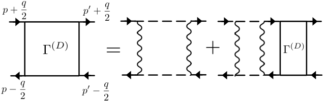

Summation over ladder diagrams is formally given as a Bethe-Salpeter equation
| (148) |
The colons indicate that and are contracted with the tensor product of . We keep the same notation as in the text that all Green’s functions represent their disorder average. decomposes into the two-particle irreducible vertex (which is currently unspecified), plus the set of ladder diagrams connecting additional vertices by a retarded and advanced propagator. In Fourier space, we find the less abstract form
| (149) |
Since we are interested in contributions to that diverge in the limit , we have replaced the first on the right with its value .
When all of the external legs of the reducible vertex are put on shell, we obtain the four-point function of Eq. 25. Explicitly,
| (150) |
This relation allows us to directly use our results from section IV to solve for . Looking at the small limit, we set in the Green’s functions and use the identity . Comparing to the solution for in Eq. 55, we immediately find
| (151) |
The superscript (D) emphasizes this is not the full reducible vertex, but instead its long time/length limit, the diffuson. The appearance of in the denominator is a consequence of the choice for the irreducible vertex, where is the bare irreducible vertex defined in Fig. 11. This choice generates the sum of all non-crossing box diagrams.
The cooperon is derived by first crossing all bare vertices , then individually crossing the wavy lines within each as shown in the lower half of Fig. 13. This is equivalent to a summation over all maximally crossed box diagrams. By left-right reflection of the lower lines (i.e. reversing all of the arrows), we can un-cross the box diagrams, thereby obtaining an identical set of ladder diagrams as used for the diffuson. The new wavenumbers are reversed and of opposite sign. We thus find the cooperon
| (152) |
Finally, we note that by including cooperon insertions into the ladder diagrams defining the diffuson Vollhardt and Wölfle 1992, we find corrections to the diffusion coefficient that recover the weak localization calculation of section V.
Appendix E Full analytic expressions
E.1
| (153) |
| (154) |
| (155) |
| (156) |
| (157) |
E.2
| (158) |
| (159) |
| (160) |
| (161) |
| (162) |
| (163) |
E.3
| (164) |
| (165) |
| (166) |
| (167) |
| (168) |
| (169) |
| (170) |
| (171) |
| (172) |
| (173) |
| (174) |
| (175) |
References
- Kearey et al. (2009) P. Kearey, K. A. Klepeis, and F. J. Vine, Global Tectonics (John Wiley & Sons, 2009).
- Wang and Hu (2005) L. Wang and H. Hu, Phys. Rev. B 71, 195412 (2005).
- Bower et al. (1999) C. Bower, R. Rosen, L. Jin, J. Han, and O. Zhou, Appl. Phys. Lett. 74, 3317 (1999).
- Vaziri and Mahadevan (2008) A. Vaziri and L. Mahadevan, Proc. Natl. Acad. Sci. U.S.A. 105, 7913 (2008).
- Lazarus et al. (2012) A. Lazarus, H. Florijn, and P. M. Reis, Phys. Rev. Lett. 109, 144301 (2012).
- Bende et al. (2015) N. P. Bende, A. A. Evans, S. Innes-Gold, L. A. Marin, I. Cohen, R. C. Hayward, and C. D. Santangelo, Proc. Natl. Acad. Sci. U.S.A. 112, 11175 (2015).
- Waugh and Evans (1979) R. Waugh and E. Evans, Biophysical Journal 26, 115 (1979).
- Park et al. (2010) Y. Park, C. A. Best, K. Badizadegan, R. R. Dasari, M. S. Feld, T. Kuriabova, M. L. Henle, A. J. Levine, and G. Popescu, Proc. Natl. Acad. Sci. U.S.A. 107, 6731 (2010).
- Park et al. (2011) Y. Park, C. A. Best, T. Kuriabova, M. L. Henle, M. S. Feld, A. J. Levine, and G. Popescu, Phys. Rev. E 83, 051925 (2011).
- Lidmar et al. (2003) J. Lidmar, L. Mirny, and D. R. Nelson, Phys. Rev. E 68, 051910 (2003).
- Ivanovska et al. (2004) I. Ivanovska, P. De Pablo, B. Ibarra, G. Sgalari, F. MacKintosh, J. Carrascosa, C. Schmidt, and G. Wuite, Proc. Natl. Acad. Sci. U.S.A. 101, 7600 (2004).
- Kuriabova and Levine (2008) T. Kuriabova and A. J. Levine, Phys. Rev. E 77, 031921 (2008).
- Michel et al. (2006) J. Michel, I. Ivanovska, M. Gibbons, W. Klug, C. Knobler, G. Wuite, and C. Schmidt, Proc. Natl. Acad. Sci. U.S.A. 103, 6184 (2006).
- Klug et al. (2006) W. S. Klug, R. F. Bruinsma, J.-P. Michel, C. M. Knobler, I. L. Ivanovska, C. F. Schmidt, and G. J. Wuite, Phys. Rev. Lett. 97, 228101 (2006).
- Dervaux and Amar (2008) J. Dervaux and M. B. Amar, Phys. Rev. Lett. 101, 068101 (2008).
- Radzihovsky and Nelson (1991) L. Radzihovsky and D. R. Nelson, Phys. Rev. A 44, 3525 (1991).
- Morse and Lubensky (1992) D. C. Morse and T. C. Lubensky, Phys. Rev. A 46, 1751 (1992).
- Radzihovsky and Le Doussal (1992) L. Radzihovsky and P. Le Doussal, Journal de Physique I 2, 599 (1992).
- Le Doussal and Radzihovsky (1993) P. Le Doussal and L. Radzihovsky, Phys. Rev. B 48, 3548 (1993).
- Evans et al. (2017) A. A. Evans, B. Bhaduri, G. Popescu, and A. J. Levine, Proc. Natl. Acad. Sci. U.S.A. 114, 2865 (2017).
- Evans and Levine (2013) A. A. Evans and A. J. Levine, Phys. Rev. Lett. 111, 038101 (2013).
- Ishimaru (2017) A. Ishimaru, Electromagnetic Wave Propagation, Radiation, and Scattering: from Fundamentals to Applications (John Wiley & Sons, 2017).
- Akkermans and Montambaux (2007) E. Akkermans and G. Montambaux, Mesoscopic Physics of Electrons and Photons (Cambridge university press, 2007).
- Rammer (2018) J. Rammer, Quantum Transport Theory (CRC Press, 2018).
- van Rossum and Nieuwenhuizen (1999) M. v. van Rossum and T. M. Nieuwenhuizen, Reviews of Modern Physics 71, 313 (1999).
- Sheng (2006) P. Sheng, Introduction to Wave Scattering, Localization and Mesoscopic Phenomena, Vol. 88 (Springer Science & Business Media, 2006).
- Chakravarty and Schmid (1986) S. Chakravarty and A. Schmid, Physics Reports 140, 193 (1986).
- Campillo and Paul (2003) M. Campillo and A. Paul, Science 299, 547 (2003).
- Korn (1993) M. Korn, Journal of Applied Geophysics 29, 247 (1993).
- Bayer and Niederdränk (1993) G. Bayer and T. Niederdränk, Phys. Rev. Lett. 70, 3884 (1993).
- Vollhardt and Wölfle (1992) D. Vollhardt and P. Wölfle, in Modern Problems in Condensed Matter Sciences, Vol. 32 (Elsevier, 1992) pp. 1–78.
- Barabanenkov and Ozrin (1991) Y. N. Barabanenkov and V. Ozrin, Physics Letters A 154, 38 (1991).
- Akkermans and Maynard (1985) E. Akkermans and R. Maynard, Journal de Physique Lettres 46, 1045 (1985).
- Wolf and Maret (1985) P.-E. Wolf and G. Maret, Phys. Rev. Lett. 55, 2696 (1985).
- Van Albada and Lagendijk (1985) M. P. Van Albada and A. Lagendijk, Phys. Rev. Lett. 55, 2692 (1985).
- Anderson (1958) P. W. Anderson, Physical Review 109, 1492 (1958).
- Thouless (1974) D. J. Thouless, Physics Reports 13, 93 (1974).
- Košmrlj and Nelson (2013) A. Košmrlj and D. R. Nelson, Phys. Rev. E 88, 012136 (2013).
- Košmrlj and Nelson (2014) A. Košmrlj and D. R. Nelson, Phys. Rev. E 89, 022126 (2014).
- Nelson et al. (2004) D. R. Nelson, T. Piran, and S. Weinberg, Statistical Mechanics of Membranes and Surfaces (World Scientific, 2004).
- Larche et al. (1986) F. C. Larche, J. Appell, G. Porte, P. Bassereau, and J. Marignan, Phys. Rev. Lett. 56, 1700 (1986).
- Safinya et al. (1986) C. R. Safinya, D. Roux, G. S. Smith, S. K. Sinha, P. Dimon, N. A. Clark, and A. M. Bellocq, Phys. Rev. Lett. 57, 2718 (1986).
- Niordson (2012) F. I. Niordson, Shell Theory (Elsevier, 2012).
- Frankel (2011) T. Frankel, The Geometry of Physics: an Introduction (Cambridge university press, 2011).
- Nelson and Peliti (1987) D. Nelson and L. Peliti, Journal de Physique 48, 1085 (1987).
- John et al. (1983) S. John, H. Sompolinsky, and M. J. Stephen, Phys. Rev. B 27, 5592 (1983).
- Kirkpatrick (1985) T. Kirkpatrick, Phys. Rev. B 31, 5746 (1985).
- McKane and Stone (1981) A. McKane and M. Stone, Annals of Physics 131, 36 (1981).
- Altland and Simons (2010) A. Altland and B. D. Simons, Condensed Matter Field Theory (Cambridge university press, 2010).
- Kroha et al. (1993) J. Kroha, C. Soukoulis, and P. Wölfle, Phys. Rev. B 47, 11093 (1993).
- van Albada et al. (1991) M. P. van Albada, B. A. van Tiggelen, A. Lagendijk, and A. Tip, Phys. Rev. Lett. 66, 3132 (1991).
- van Tiggelen et al. (1992) B. A. van Tiggelen, A. Lagendijk, M. P. van Albada, and A. Tip, Phys. Rev. B 45, 12233 (1992).
- (53) This name was chosen to agree with the nomenclature used for this approximation in computing the conductivity of a metal. See Ref. Akkermans and Montambaux 2007 for more details.
- Le Doussal and Radzihovsky (1992) P. Le Doussal and L. Radzihovsky, Phys. Rev. Lett. 69, 1209 (1992).
- Zakharchenko et al. (2010) K. V. Zakharchenko, R. Roldán, A. Fasolino, and M. I. Katsnelson, Phys. Rev. B 82, 125435 (2010).
- Gazit (2009) D. Gazit, Phys. Rev. E 80, 041117 (2009).
- Schwartz (2014) M. D. Schwartz, Quantum Field Theory and the Standard Model (Cambridge University Press, 2014).