Elastic Wave Near-Cloaking

First, we set the scene using anti-plane shear waves where the displacement $U_{3}(X_{1},X_{2})$ is governed by the two-dimensional scalar wave equation:

$$\bar{\nabla}_{\boldsymbol{X}}\cdot(\mu_{0}\bar{\nabla}_{\boldsymbol{X}}U_{3})=\rho_{0}\frac{\partial^{2}U_{3}}{\partial t^{2}}$$

(4)

with $\bar{\nabla}_{\boldsymbol{X}}$ as the differential operator in two dimensions, $\mu_{0}$ and $\rho_{0}$ the shear modulus and the mass density, respectively; for homogeneous media (4) is:

$$\bar{\nabla}_{\boldsymbol{X}}^{2}U_{3}=\frac{1}{c_{S0}^{2}}\frac{\partial^{2}U_{3}}{\partial t^{2}}$$

(5)

with shear wavespeed $c_{S0}=\sqrt{\displaystyle\frac{\mu_{0}}{\rho_{0}}}$. Applying the conformal map (3) then gives

$$\bar{\nabla}^{2}u_{3}=\frac{1}{n^{2}c_{S0}^{2}}\frac{\partial^{2}u_{3}}{\partial t^{2}}$$

(6)

where $u_{3}(\boldsymbol{x}(\boldsymbol{X}))=U_{3}(\boldsymbol{X})$. It is now possible to deduce a new material, occupying the domain $\xi$, with shear modulus $\mu$ and density $\rho$ such that it mimics the virtual domain. The wave equation governing its anti-plane motion reads:

$$\bar{\nabla}\mu\cdot\bar{\nabla}u_{3}+\mu\bar{\nabla}^{2}u_{3}=\rho\frac{\partial^{2}u_{3}}{\partial t^{2}}$$

(7)

and if the gradient of $\mu$ is null, then it is sufficient that

$$\displaystyle\frac{\mu}{\rho}=n^{2}c_{S0}^{2}$$

for the medium to mimic the virtual domain. In particular, selecting material properties $\mu=\mu_{0}$ and $\rho={\rho_{0}}/{n^{2}}$ gives the perfect conformal cloak and this process mirrors that in electromagnetism or acoustics [44, 45].

We now turn our attention to the full vector equations of elastodynamics that do not allow the neat process in the previous section to be performed exactly. The vector displacement $\boldsymbol{U}$ in homogeneous media obeys the elastodynamic Navier wave equation [46]:

$$(\lambda_{0}+2\mu_{0})\nabla_{\boldsymbol{X}}(\nabla_{\boldsymbol{X}}\cdot\boldsymbol{U})-\mu_{0}\nabla_{\boldsymbol{X}}\times\nabla_{\boldsymbol{X}}\times\boldsymbol{U}=\rho_{0}\frac{\partial^{2}\boldsymbol{U}}{\partial t^{2}}$$

(8)

with $\lambda_{0}$ and $\mu_{0}$ the Lamè parameters of the material. The Helmholtz decomposition

$$\boldsymbol{U}=\nabla_{\boldsymbol{X}}\Phi+\nabla_{\boldsymbol{X}}\times\boldsymbol{\Psi},\quad\nabla_{\boldsymbol{X}}\cdot\boldsymbol{\Psi}=0$$

(9)

using the scalar compressional $\Phi$, and vector shear $\boldsymbol{\Psi}$, potentials gives two wave equations:

$$\nabla_{\boldsymbol{X}}^{2}\Phi=\frac{1}{c_{P0}^{2}}\frac{\partial^{2}\Phi}{\partial t^{2}},\qquad\nabla_{\boldsymbol{X}}^{2}\Psi_{i}=\frac{1}{c_{S0}^{2}}\frac{\partial^{2}\Psi_{i}}{\partial t^{2}}\qquad i=1,2,3$$

(10)

with compressional wavespeed $c_{P0}^{2}=({\lambda_{0}+2\mu_{0}})/{\rho_{0}}$ and shear wavespeed $c_{S0}^{2}={\mu_{0}}/{\rho_{0}}$. At first sight these appear as decoupled wave equations and naively applying the same process, using the conformal map, as in anti-plane elasticity appears attractive. In terms of an exact solution this idea is flawed as traction-free boundary conditions implicitly couple the potentials.

We consider plane wave propagation in the $X_{1},X_{2}$ plane: an harmonic P-wave and shear waves are obtained from

$$\Phi(\boldsymbol{X},t)=\Phi_{0}e^{j(\omega t-\boldsymbol{\kappa}\cdot\boldsymbol{X})},\qquad\boldsymbol{\Psi}(\boldsymbol{X},t)=\boldsymbol{\Psi}_{0}e^{j(\omega t-\boldsymbol{\kappa}\cdot\boldsymbol{X})}$$

(11)

respectively. We align our axes so that for plane wave propagation no gradients are observed in the third direction, and the problem is then essentially two-dimensional, and the wave equation for the scalar potential becomes:

$$\bar{\nabla}_{\boldsymbol{X}}^{2}\Phi=\frac{1}{c_{P0}^{2}}\frac{\partial^{2}\Phi}{\partial t^{2}}$$

(12)

Moreover, the displacements associated with shear waves, are expressed in terms of $\boldsymbol{\Psi}$ as

$$\boldsymbol{U}=\nabla_{\boldsymbol{X}}\times\boldsymbol{\Psi}=\begin{bmatrix}\Psi_{3,2}\\ -\Psi_{3,1}\\ \Psi_{2,1}-\Psi_{1,2}\end{bmatrix}$$

(13)

For a SV wave there is no antiplane motion thus:

$$\Psi_{2,1}-\Psi_{1,2}=0$$

(14)

and without loss of generality $\Psi_{1}$ and $\Psi_{2}$ are taken zero, thus the vector wave equation governing plane shear waves is the two-dimensional scalar wave equation in $\Psi_{3}$:

$$\bar{\nabla}_{\boldsymbol{X}}^{2}\Psi_{3}=\frac{1}{c_{S0}^{2}}\frac{\partial^{2}\Psi_{3}}{\partial t^{2}}$$

(15)

To summarise, the equations for in-plane motion are:

$$\bar{\nabla}_{\boldsymbol{X}}^{2}\Phi=\frac{1}{c_{P0}^{2}}\frac{\partial^{2}\Phi}{\partial t^{2}},\qquad\bar{\nabla}_{\boldsymbol{X}}^{2}\Psi_{3}=\frac{1}{c_{S0}^{2}}\frac{\partial^{2}\Psi_{3}}{\partial t^{2}}.$$

(16)

As previously seen in section 2.1, after transformation, these equations become

$$\bar{\nabla}^{2}\phi=\frac{1}{n^{2}c_{P0}^{2}}\frac{\partial^{2}\psi}{\partial t^{2}},\qquad\bar{\nabla}^{2}\psi_{3}=\frac{1}{n^{2}c_{S0}^{2}}\frac{\partial^{2}\phi_{3}}{\partial t^{2}}.$$

(17)

To find the corresponding material properties that, in the physical domain, mimic the wave propagation occurring in virtual domain, we now consider the elastodynamic wave equations for general inhomogeneous media:

$$\begin{split}&\nabla\lambda(\nabla\cdot\boldsymbol{u})+\nabla\mu\cdot[\nabla\boldsymbol{u}+(\nabla\boldsymbol{u})^{T}]+\\ &+(\lambda+2\mu)\nabla(\nabla\cdot\boldsymbol{u})-\mu\nabla\times\nabla\times\boldsymbol{u}=\rho\frac{\partial^{2}{\boldsymbol{u}}}{\partial t^{2}}.\end{split}$$

(18)

If the gradient of the Lamé parameters is null, upon the substitution:

$$\boldsymbol{u}=\nabla\phi+\nabla\times\boldsymbol{\psi}$$

(19)

the following is obtained:

$$\begin{split}&(\lambda+2\mu)\nabla(\nabla^{2}\phi)-\rho\frac{\partial^{2}}{\partial t^{2}}\nabla\phi=\\ &=-\left[\mu\nabla\times\nabla^{2}\boldsymbol{\psi}-\rho\frac{\partial^{2}}{\partial t^{2}}(\nabla\times\boldsymbol{\psi})\right]\end{split}$$

(20)

This is rearranged as:

$$\begin{split}&\nabla\left[(\lambda+2\mu)\nabla^{2}\phi-\rho\frac{\partial^{2}\phi}{\partial t^{2}}\right]+\nabla\rho\frac{\partial^{2}\phi}{\partial t^{2}}=\\ &=\nabla\times\left[\mu\nabla^{2}\boldsymbol{\psi}-\rho\frac{\partial^{2}\boldsymbol{\psi}}{\partial t^{2}}\right]+\nabla\rho\times\frac{\partial^{2}\boldsymbol{\psi}}{\partial t^{2}}\end{split}$$

(21)

thus, if the gradient of density can be considered negligible, then the identity is satisfied by

$$\begin{split}&(\lambda+2\mu)\nabla^{2}\phi-\rho\frac{\partial^{2}\phi}{\partial t^{2}}=0\\ &\mu\nabla^{2}\boldsymbol{\psi}-\rho\frac{\partial^{2}\boldsymbol{\psi}}{\partial t^{2}}=0\end{split}$$

(22)

and the same decomposition in scalar and vector potentials is seen to be applied as in the case of the virtual domain. The cloak for plane waves can then be performed by scaling both longitudinal and transversal wave speeds according to the local metric change of the transformation. The displacements will be then associated to the gradient of $\phi$ and to the curl of $\boldsymbol{\psi}$.

$$\boldsymbol{u}=\nabla\phi+\nabla\times\boldsymbol{\psi}$$

(23)

since for the chain rule $\nabla=\boldsymbol{F}^{-T}\nabla_{\boldsymbol{X}}$, then, recalling that $\boldsymbol{V}\in\mathrm{Sym}^{+}$ is symmetric and $\boldsymbol{R}$ is orthogonal:

$$\boldsymbol{u}=\boldsymbol{F}^{-T}\boldsymbol{U}=\boldsymbol{V}^{-1}\boldsymbol{R}\boldsymbol{U}=\frac{1}{n}\boldsymbol{R}\boldsymbol{U}$$

(24)

This means that the displacements assume the same local rotation of the medium and are simply scaled according to the local stretch.

Clearly an assumption has been made above regarding the density gradient and we now assess and quantify the impact, and limitations, of doing so, by obtaining a global performance index for the cloak. Turning to Eq. (21): considering the term proportional to $\nabla\rho$ as being negligible, is also interpreted as adding an extra term to each side of (20), such that the the left hand side is rewritten as:

$$(\lambda+2\mu)\nabla(\nabla^{2}\phi)-\rho\frac{\partial^{2}}{\partial t^{2}}\nabla\phi-\nabla\rho\frac{\partial^{2}\phi}{\partial t^{2}}$$

(25)

while the right hand side becomes:

$$-\left[\mu\nabla\times\nabla^{2}\boldsymbol{\psi}-\rho\frac{\partial^{2}}{\partial t^{2}}(\nabla\times\boldsymbol{\psi})-\nabla\rho\times\frac{\partial^{2}\boldsymbol{\psi}}{\partial t^{2}}\right]$$

(26)

We use the relation for plane waves in homogeneous media $\phi=\hat{\phi}e^{i(\omega t-\boldsymbol{\kappa}_{P}\cdot\boldsymbol{x})}$ to make estimates of the modulus of the last two terms in (25):

$$\left|\rho\frac{\partial^{2}}{\partial t^{2}}\nabla\phi\right|\approx\rho_{0}\omega^{2}\kappa_{P}\hat{\phi};\qquad\left|\nabla\rho\frac{\partial^{2}\phi}{\partial t^{2}}\right|\approx<\nabla\rho>\omega^{2}\hat{\phi}$$

(27)

having introduced $<\nabla\rho>$, i.e. the averaged value of the gradient of density over the surface of the cloak, as an estimate of $\nabla\rho$. The order of magnitude of the ratio between the two is:

$$O\left(\frac{<\nabla\rho>/\rho_{0}}{\kappa_{P}}\right)=O\left(\frac{<1/n^{2}>c_{P}}{2\pi f}\right)$$

(28)

which shows this added extra term can be reasonably considered negligible in the limit where $\kappa_{P}$ becomes very large and/or the fluctuation in density with respect to background value (i.e. the fluctuations of metric change) are small. A similar approach applies for the last two terms in (26): assuming $\boldsymbol{\psi}=\hat{\boldsymbol{\psi}}e^{i(\omega t-\boldsymbol{\kappa}_{S}\cdot\boldsymbol{x})}$ the modulus of the related terms become:

$$\left|\rho\frac{\partial^{2}}{\partial t^{2}}(\nabla\times\boldsymbol{\psi})\right|\approx\rho_{0}\omega^{2}\kappa_{S}|\hat{\boldsymbol{\psi}}|;\quad\left|\nabla\rho\times\frac{\partial^{2}\boldsymbol{\psi}}{\partial t^{2}}\right|\approx<\nabla\rho>\omega^{2}|\hat{\boldsymbol{\psi}}|$$

(29)

which means the ratio scales as

$$O\left(\frac{<\nabla\rho>/\rho_{0}}{\kappa_{S}}\right)=O\left(\frac{<1/n^{2}>c_{S}}{2\pi f}\right)$$

(30)

As a consequence, for a given transformation the cloak is expected to have increasingly good performances for all frequencies above a certain cutoff, which is set from the conditions expressed by requiring the adimensional ratios (28) and (30) being small. Note that, since the wavelength of P waves is always longer than that of shear waves ($c_{P}>c_{S}$), the condition set by $\kappa_{P}$ is the one that is more demanding. The difference between (28) and (30) only depends on the ratio of wave speeds, that in turn depends only on Poisson’s ratio. Reducing $\nu$ results in a reduced difference between $c_{P}$ and $c_{S}$, thus reduced difference between the performance of the cloak with respect to the two types of waves.

Note that the same distribution of refraction index could be in principle obtained keeping fixed the density and scaling both the Lamè parameters or even changing all the three material parameters, as proposed in previous works [39], [40]. However, following the previous analysis, it is clearly less convenient to change both Lamé parameters and density at the same time, because further approximations will be introduced in passing from (18) to (20), other than those that were just analyzed. Moreover, if modulation of the stiffness properties is adopted instead of the density, according to (7), some non idealities will be introduced in the anti-plane solution also, which is instead perfect when density modulation only is considered.

We now exploit the insight gained from our theory to obtain a carpet cloak working for both in-plane and anti-plane motion. A height defect with Gaussian shape on an otherwise flat free surface is probed by an incident wave. The conformal map linking such deformed domain to the reference flat surface is shown in Figure 6 and used to evaluate the local metric deformation $n$. As discussed earlier such a stretch corresponds to the refraction index of both P and S wave speeds, and the cloak is simply obtained by scaling the density of the material around the obstacle. A nuance is that the conformal map is defined on the whole semi-infinite space, whereas the cloak has to be finite in size. This issue is simply addressed by truncating the cloak sufficiently far from the obstacle to let the stretch approach unity.

To validate the expected cloaking performances, we perform numerical finite element simulations of the full Navier equations based on the scattering formulation [5]. The mesh is designed to have at least twelve quadratic elements per minimum wavelength involved in the simulation to ensure convergence. The background material is a polymer characterized by Young’s modulus $E=3$ [GPa], Poisson’s ratio $\nu=0.4$ and density $\rho=1190$ [kg/m³]. Figure 7 visually displays the performance of the designed cloak at fixed frequency $f=200$ [kHz] for impinging SV and P waves at $\pi/4$ incidence. On the left side of Figure 7 the magnitude of the displacement field is depicted for the reference case, the plain obstacle, and the obstacle surrounded with the cloak, for a SV impinging wave. Each simulation is accompanied by the 2D fast Fourier transform (FFT) of the displacement field, that displays in wavenumber space the scattering directions. Each FFT is normalized with respect to its maximum, in order to clearly show all the directions of scattering. It is clearly seen that the cloak is able to conceal the presence of the Gaussian defect of the surface, which otherwise would scatter energy in almost every direction, with symmetric peaks at each side of the expected reference reflection direction. On the right side of Figure 7, the P wave case is shown. For both SV and P waves mode conversion can occur at a free surface, i.e, a transverse wave can be reflected as both a transverse and a longitudinal wave and, in the same way, a longitudinal wave can produce scattered waves with both polarizations. Such mode conversion obeys Snell’s law, meaning that

$$c_{i}\sin{\theta_{i}}=c_{r}\sin{\theta_{r}}$$

(31)

with $\theta_{i}$, $\theta_{r}$ the incidence and reflection angles, and $c_{i}$, $c_{r}$ the speeds of the incident and reflected waves. As a consequence, the reflection angle associated to a SV wave will always be less than that associated to a P wave, $c_{S}$ being less than $c_{P}$. This in turn reflects that, for a 45 degree incident shear wave, no reflected P wave is expected, as seen from the reference and cloaked cases. The bare obstacle, instead, besides scattering transverse waves in several directions, also generates some mode conversion. Indeed the amplitude of the FFT is different from zero also for normalized $\kappa/\kappa_{S}\approx 0.4$ which corresponds to the ratio of P to SV wavenumbers. The impinging P wave case clearly shows the conversion of polarizations, which can also be seen through the appearance of two strong spots in the FFT of the reference and cloaked cases. As in the other case, the obstacle scatters energy almost in all directions.

The dependence of the cloak performance on angle of incidence, $\theta_{i}$, is shown in figure 8. For each $\theta_{i}$ the cloaked and bare obstacle are compared in terms of the distribution of the FFT calculated for wavenumbers corresponding to P and S waves (the white quarter of circles depicted in Figure 7), which is plotted together with the related reflection direction $\theta_{r}=\arctan(\kappa_{2}/\kappa_{1})$. This allows us to assess whether most of the signal is concentrated on the expected reflection angle (marked with dashed blue lines) or whether it is spread over a wide range of angles, and allows us to better appreciate the reduction of mode conversion.

The dependence of cloaking performance with respect to frequency of operation and maximum width of the Gaussian defect are completely defined by the indicators given by (28) and (30). Referring to the most demanding indicator, the calculated order of magnitude for the case shown in Figure 6 is:

$$\frac{<\nabla\rho>/\rho_{0}}{\kappa_{P}}\approx 0.017$$

(32)

A thorough numerical sensitivity analysis of the performance of the cloak with respect to changes in this global indicator are given in the Supplementary Material.

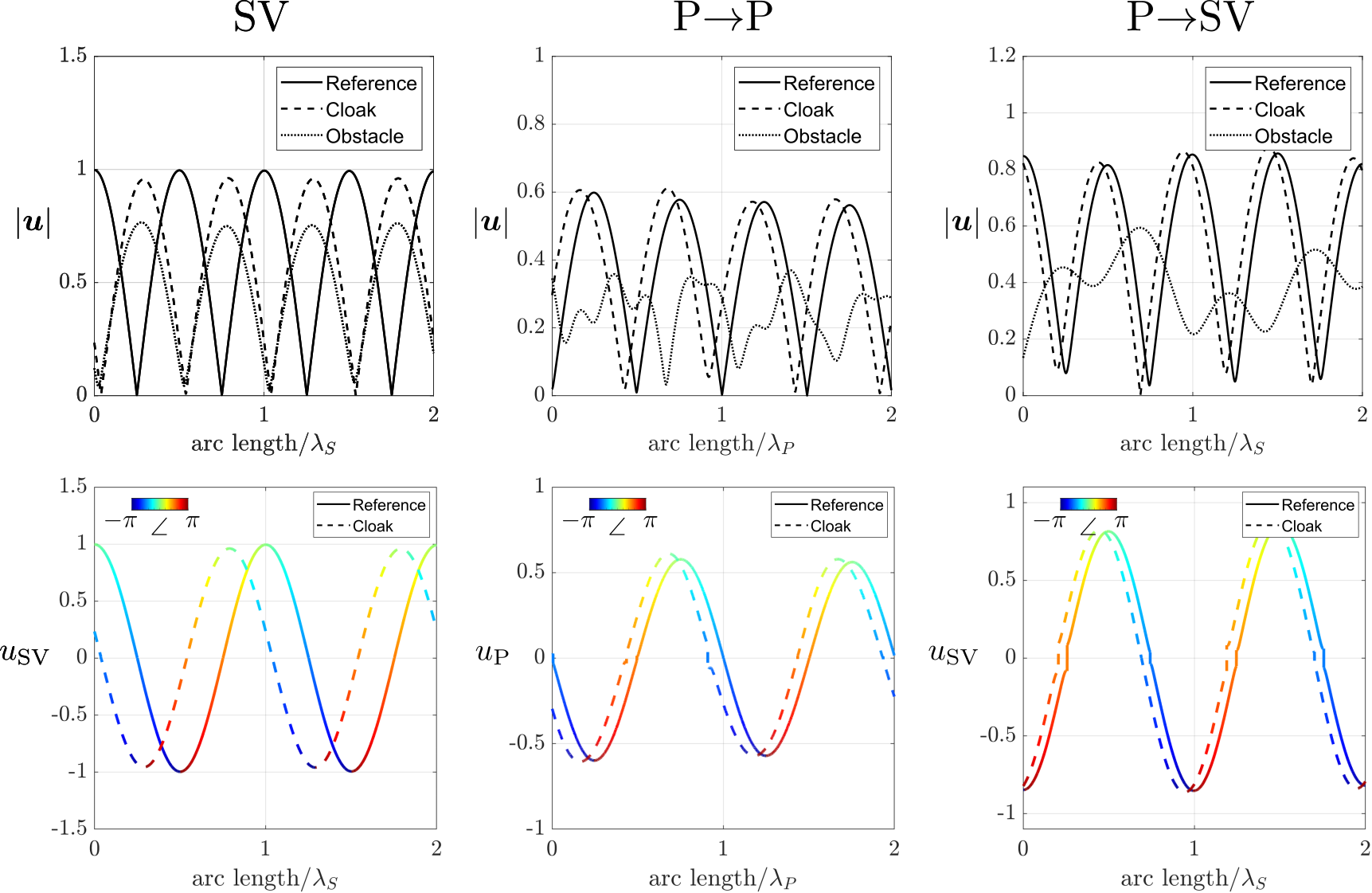
As the cloak is finite, a phase shift is also expected between the reference and cloak solutions. This is hard to discern from the field plots shown in Figure 7 and hence we show solutions evaluated along the travelling direction of the scattered waves along the red lines shown in the lower panels of Figure 7 and plotted in Figure 9. On the bottom line, from left to right we show a comparison between the cloak and reference solutions for an impinging SV wave, the reflected P wave from impinging P wave, and the reflected shear wave from impinging compressional one, respectively. The comparison is made in terms of the transversal displacement $u_{S}$ for the shear waves and of longitudinal displacement $u_{P}$ for compressional waves. The color indicates the phase, highlighting the phase shift in the response of the cloaked obstacle. In the top part of the Figure, the same plots are shown in terms of magnitude of displacements, and the scattered field of the bare obstacle is also added for comparison.

Apart from incident purely compressional, P, or shear, S, waves, the cloak works well for other incident fields and we now turn to the important example of incident Rayleigh surface waves [46]. Figure 10 shows the comparison of the scattering behaviour of the bare obstacle and the cloaked obstacle when a Rayleigh wave tries to propagate across the deformed surface. In the uncloaked scenario substantial mode conversion occurs, and additionally part of the energy is scattered into the bulk of the material as a transverse SV wave, whereas the cloak considerably reduces such scattering, allowing the signal to propagate past the surface defect as if it was not there. The critical measure of performance is not the angle of scattering, but is now the difference in total amount of energy that is converted into bulk waves and this can be visualised via the FFT and in Figure 10 the FFT of all the three cases have been normalized over the peak value of the obstacle case; this shows that remarkably little energy is scattered into the bulk by the cloaked solution.

References

- [1] M. Kadic, M. Wegener, A. Nicolet, F. Zolla, S. Guenneau, A. Diatta, Elastodynamic behavior of mechanical cloaks designed by direct lattice transformations, Wave Motion 92 (2020) 102419.
- [2] G. Milton, M. Briane, J. Willis, On cloaking for elasticity and physical equations with a transformation invariant form, New J. Phys. 8 (2006) 248.
- [3] A. N. Norris, Acoustic cloaking theory, Proceedings of the Royal Society A 464 (2008) 2411–2434.
- [4] A. N. Norris, A. L. Shuvalov, Elastic cloaking theory, Wave Motion 48 (2011) 525 – 538.
- [5] A. Diatta, M. Kadic, M. Wegener, S. Guenneau, Scattering problems in elastodynamics, Physical Review B 94 (10) (2016) 100105.
- [6] T. Bückmann, M. Thiel, M. Kadic, R. Schittny, M. Wegener, An elasto-mechanical unfeelability cloak made of pentamode metamaterials, Nature communications 5 (1) (2014) 1–6.
- [7] G. W. Milton, A. V. Cherkaev, Which elasticity tensors are realizable?, J. Eng. Mater.-T. 117 (1995) 483–493.
- [8] M. Kadic, T. Bückmann, N. Stenger, M. Thiel, M. Wegener, On the practicability of pentamode mechanical metamaterials, Appl. Phys. Lett. 100 (2012) 191901.
- [9] A. N. Norris, W. J. Parnell, Hyperelastic cloaking theory: transformation elasticity with pre-stressed solids, Proceedings of the Royal Society A 468 (2146) (2012) 2881–2903.
- [10] W. J. Parnell, A. N. Norris, T. Shearer, Employing pre-stress to generate finite cloaks for antiplane elastic waves, Applied Physics Letters 100 (17) (2012) 171907.
- [11] W. J. Parnell, Nonlinear pre-stress for cloaking from antiplane elastic waves, Proceedings of the Royal Society A: Mathematical, Physical and Engineering Sciences 468 (2138) (2012) 563–580.
- [12] X. Xu, C. Wang, W. Shou, Z. Du, Y. Chen, B. Li, W. Matusik, N. Hussein, G. Huang, Physical realization of elastic cloaking with a polar material, Phys. Rev. Lett. 124 (2020) 114301.
- [13] D. Misseroni, A. B. Movchan, D. Bigoni, Omnidirectional flexural invisibility of multiple interacting voids in vibrating elastic plates, Proc. R. Soc. Lond. A. 475 (2019) 20190283.
- [14] H. Lamb, Hydrodynamics, University Press, 1895.
- [15] L. Dolin, To the possibility of comparison of three-dimensional electromagnetic systems with nonuniform anisotropic filling, Izv. Vyssh. Uchebn. Zaved. Radiofizika 4 (5) (1961) 964–967.
- [16] J.-F. Imhoff, On original solution for unbounded electromagnetic 2D and 3D- problems throughout the finite element method, IEEE T. Magn. 26 (1990) 1659 – 1661.
- [17] A. Nicolet, J. F. Remacle, B. Meys, A. Genon, W. Legros, Transformation methods in computational electromagnetism, J. Appl. Phys. 75 (1994) 6036–6038.
- [18] J.-P. Berenger, A perfectly matched layer for the absorption of electromagnetic waves, J. Comput. Phys. 114 (1994) 185–200.
- [19] J. B. Pendry, D. Schurig, D. R. Smith, Controlling electromagnetic fields, Science 312 (2006) 1780–1782.
- [20] U. Leonhardt, Optical conformal mapping, Science 312 (2006) 1777–1780.
- [21] M. Farhat, S. Enoch, S. Guenneau, A. B. Movchan, Broadband cylindrical acoustic cloak for linear surface waves in a fluid, Phys. Rev. Lett. 101 (2008) 134501.
- [22] M. Farhat, S. Guenneau, S. Enoch, Ultrabroadband elastic cloaking in thin plates, Phys. Rev. Lett. 103 (2009) 024301.
- [23] S. A. Cummer, B.-I. Popa, D. Schurig, D. R. Smith, J. Pendry, M. Rahm, A. Starr, Scattering theory derivation of a 3d acoustic cloaking shell, Phys. Rev. Lett. 100 (2008) 024301.
- [24] S. A. Cummer, J. Christensen, A. Alù, Controlling sound with acoustic metamaterials, Nature Reviews Materials 1 (3) (2016) 16001.
- [25] B.-I. Popa, L. Zigoneanu, S. A. Cummer, Experimental acoustic ground cloak in air, Phys. Rev. Lett. 106 (2011) 253901.
- [26] D. Torrent, A. Håkansson, F. Cervera, J. Sánchez-Dehesa, Homogenization of two-dimensional clusters of rigid rods in air, Phys. Rev. Lett. 96 (2006) 204302.
- [27] D. Torrent, J. Sánchez-Dehesa, Effective parameters of clusters of cylinders embedded in a nonviscous fluid or gas, Phys. Rev. B 74 (2006) 224305.
- [28] D. Torrent, J. Sánchez-Dehesa, Acoustic cloaking in two dimensions: a feasible approach, New J. Phys. 10 (6) (2008) 063015.
- [29] D. Torrent, J. Sánchez-Dehesa, Anisotropic mass density by two-dimensional acoustic metamaterials, New J. Phys. 10 (2) (2008) 023004.
- [30] M. Farhat, S. Guenneau, S. Enoch, A. B. Movchan, Negative refraction, surface modes, and superlensing effect via homogenization near resonances for a finite array of split-ring resonators, Phys. Rev. E 80 (2009) 046309.
- [31] N. Stenger, M. Wilhelm, M. Wegener, Experiments on elastic cloaking in thin plates, Phys. Rev. Lett. 108 (2012) 014301.
- [32] S. Guenneau, C. Amra, D. Veynante, Transformation thermodynamics: cloaking and concentrating heat flux, Opt. Express 20 (2012) 8207–8218.
- [33] R. Schittny, M. Kadic, S. Guenneau, M. Wegener, Experiments on transformation thermodynamics: Molding the flow of heat, Phys. Rev. Lett. 110 (2013) 195901.
- [34] Q. Ji, X. Chen, J. Liang, V. Laude, S. Guenneau, G. Fang, M. Kadic, Non-singular homogeneous polyhedral heat cloak and its realization, ES Energy and Environment 7: Special Topic on Thermal Metamaterials II (2019) 29–39.
- [35] J. Li, J. B. Pendry, Hiding under the carpet: A new strategy for cloaking, Phys. Rev. Lett. 101 (2008) 203901.
- [36] A. Alù, N. Engheta, Achieving transparency with plasmonic and metamaterial coatings, Physical Review E 72 (1) (2005) 016623.
- [37] B. Zhang, Y. Luo, X. Liu, G. Barbastathis, Macroscopic invisibility cloak for visible light, Phys. Rev. Lett. 106 (2011) 033901.
- [38] X. Chen, Y. Luo, J. Zhang, K. Jiang, J. B. Pendry, S. Zhang, Macroscopic invisibility cloaking of visible light, Nat. Commun. 2 (2011) 176.
- [39] Z. Chang, J. Hu, G. Hu, R. Tao, Y. Wang, Controlling elastic waves with isotropic materials, Applied Physics Letters 98 (12) (2011) 121904.
- [40] H. Gao, Z. Xiang, Manipulate elastic waves with conventional isotropic materials, arXiv preprint arXiv:1809.05248 (2018).
- [41] B. Banerjee, An introduction to metamaterials and waves in composites, CRC Press, 2011.
- [42] G. D. Mahan, Conformal Mapping, Springer US, Boston, MA, 2002.
- [43] A. Greenleaf, M. Lassas, G. Uhlmann, On nonuniqueness for Calderon’s inverse problem, Math. Res. Lett. 10 (2003) 685–693.
- [44] J. Li, J. B. Pendry, Hiding under the carpet: a new strategy for cloaking, Physical review letters 101 (20) (2008) 203901.
- [45] A. V. Amirkhizi, A. Tehranian, S. Nemat-Nasser, Stress-wave energy management through material anisotropy, Wave Motion 47 (8) (2010) 519–536.
- [46] K. F. Graff, Wave motion in elastic solids, Courier Corporation, 2012.
- [47] M. Kadic, T. Bückmann, R. Schittny, P. Gumbsch, M. Wegener, Pentamode metamaterials with independently tailored bulk modulus and mass density, Physical Review Applied 2 (5) (2014) 054007.
Supplementary Material
To supplement the material in the main article we perform a parametric analysis of the performance of the near-cloaking. As explained in the main article, the cloak is achieved by assuming that additional terms connected to the slow variation of density, appearing in the equation of the physical domain are negligible. These terms depend both on the frequency of operation and on the gradient of density inside the cloak. Since the gradient of density is a local property of the cloak, we have introduced a global measure of performance with the following two non-dimensional indicators: