The Stationary Points of the Hierarchical Three Body Problem2020
Abstract
We study the stationary points of the hierarchical three body problem in the planetary limit () at both the quadrupole and octupole orders. We demonstrate that the extension to octupole order preserves the principal stationary points of the quadrupole solution in the limit of small outer eccentricity but that new families of stable fixed points occur in both prograde and retrograde cases. The most important new equilibria are those that branch off from the quadrupolar solutions and extend to large . The apsidal alignment of these families is a function of mass and inner planet eccentricity, and is determined by the relative directions of precession of and at the quadrupole level. These new equilibria are also the most resilient to the destabilizing effects of relativistic precession. We find additional equilibria that enable libration of the inner planet argument of pericentre in the limit of radial orbits and recover the non-linear analogue of the Laplace-Lagrange solutions in the coplanar limit. Finally, we show that the chaotic diffusion and orbital flips identified with the Eccentric Kozai Lidov mechanism and its variants can be understood in terms of the stationary points discussed here.
Keywords:
celestial mechanics – planets and satellites: dynamical evolution and stability – methods:analytical1 Introduction
The application of the hierarchical three-body problem to planetary systems has received significant attention over the last decade, motivated by the possibility that planets discovered in short period orbits (Mayor & Queloz 1995; Dawson & Johnson 2018) may be the result of high eccentricities generated by special classes of solutions of the hierarchical problem (Innanen et al. 1997; Wu & Murray 2003; Fabrycky & Tremaine 2007; Wu et al. 2007; Veras & Ford 2010; Naoz et al. 2011; Naoz et al. 2012; Naoz et al. 2013a; Naoz 2016).
A related question is the source of the high eccentricities observed in exoplanet systems in general (Marcy et al. 1999; Marcy et al. 2005; Udry & Santos 2007). Whatever the original mechanism for eccentricity excitation is, only a subset of planetary systems are expected to undergo the extreme eccentricity growth that would enable the tidal drag-down of planets to short periods. The remainder of the population is expected to remain in a configuration set in place by the original eccentricity excitation. In some cases, this may be reflected in mean motion resonances, but many systems will exhibit oscillations in eccentricity and inclination modulated by the secular interactions between the planetary orbits.
The exoplanetary systems are complex dynamical systems that can exhibit a range of phenomena, including apsidal and nodal circulation and libration and resonances between various periodicities in the system. One way to organise this information is to study the stationary points of the dynamical system and to classify the resulting equilibria in terms of their stability. Several studies have sought to understand how observed planetary systems fall within the range of available equilibria (Michtchenko et al. 2006; Libert & Henrard 2006; Libert & Henrard 2007; Libert & Tsiganis 2009; Volpi et al. 2019). We wish to examine the full range of stationary points relevant to the hierarchical secular problem, over the full range of mass ratio and mutual inclinations, extending extant results such as those by Migaszewski & Goździewski 2009 (limited to mass ratios of order unity) and Migaszewski & Goździewski 2011 (limited to prograde mutual inclinations). Our goal is to better understand the relationship between observed systems and the dynamical pathways by which systems can evolve.
In § 2 we will review prior work on the stationary points of the hierarchical problem at quadrupolar order, and in § 3 we will extend this to the Octopolar order. We will examine the effect of corrections due to relativistic precession in § 4 and classify the stability of the identified stationary points in § 5. In § 6 we will frame several well-known features of the dynamics in terms of the identified stationary points and summarise the conclusions in § 7.
2 Quadrupolar Fixed Points
In order to establish our framework, we review here the stationary points of the hierarchical three body problem as described by the Hamiltonian expanded to quadrupole order in , the ratio of the semi-major axes of the inner and outer planets (Kozai 1962; Harrington 1968; Lidov & Ziglin 1976; Ferrer & Osacar 1994). Adopting the formulation from Naoz 2016, the equations of motion for the inner planet eccentricity, , and the inner argument of perihelion, are
| (1) | |||||
| (2) | |||||
where is a constant that depends on the masses and semi-major axes and , where is the relative inclination of the inner and outer orbital planes. The constant is the mass ratio between the inner and outer planet. This is the limiting expression in the planetary case, where and are much less massive than the central body . In the more general case, contains a prefactor .
The stationary points of the problem are found by solving for and simultaneously. The fact that the argument of periastron of the outer planet – – does not appear here (the ‘happy coincidence’ of Lidov & Ziglin 1976) means that these two criteria are sufficient. A finite value of will not affect the dynamics but can parameterise the solutions.
Examination of equation (1) establishes several possible branches of solution. The most obvious are for (we will call this case ) and (we will call this case ). However, there are also a set of limiting cases that may also apply. This equation is also satisfied in the case of circular ( – case ), radial ( – case ) or coplanar ( – case ). Let us discuss each in turn (Table 1 presents a summary).
2.1 Case :
By setting in equation (2), the condition for a stationary point is
| (3) |
We see that this family of stationary points only applies for retrograde orbits ( always) and only for large enough mass ratios, since implies for , which is when the family of stationary points first manifests itself.
2.2 Case :
In this case, setting yields a quadratic solution for in terms of .
| (4) |
This condition defines the stationary point corresponding to the well-known Kozai-Lidov librations (Kozai 1962; Lidov 1962). The low mass () limit asymptotes to the solution from the original (inner test particle) formulation by Kozai & Lidov,
| (5) |
In the opposite limit of large , this family of stationary points becomes asymmetric and the prograde and retrograde branches have different asymptotes, namely
| (6) |
which tends to polar orbits (regardless of ) in the limit of an outer test particle (Ziglin 1975), and
| (7) |
which becomes unphysical (because is large) unless is close enough to radial. Thus, the retrograde stationary points only exist for almost radial orbits in the large mass ratio limit.
Given this asymmetry at high mass ratios, we will adopt separate labels for the prograde () and retrograde () parts of the stationary point family.
| Name | Orbit | Comments | |
|---|---|---|---|
| Retrograde | Saddle Point | ||
| Prograde | all | Fixed Point | |
| Retrograde | all | Fixed Point | |
| Both | all | Saddle Point | |
| Polar | all | Saddle Point | |
| Retrograde | Saddle Point |
2.3 Case :
An alternative path to satisfy is to set in equation (1). In this case, it does not impose a condition on , as in the previous two sections. Instead, we must constrain by setting equation (2) to zero, which yields
| (8) |
We will discuss the meaning of this equation in § 2.7, but it is worth noting here that setting yields the same equation as the circular limit of equation (3), and setting yields the same equation as the circular limit of equation (4).
2.4 Case :
To satisfy for we require both and or . This case is therefore a very localised stationary point – in the limit of polar, radial orbits.
2.5 Case :
Setting and in Eqs. (1) and (2), in the prograde, coplanar () case, we do not find any any physical solutions. For the case , these equations yield the condition
| (9) |
This equation yields physically realistic solutions () for and has the same limit as Case , suggesting a common link between these cases.
2.6 Precession of the Outer Body
Although the evolution of the system, to quadrupolar order, does not depend on , this variable will come into play when we extend our analysis to octupole order. Therefore, the condition , at quadrupolar order, will become relevant. In the case of , this leads to the condition
| (10) |
which has the solution
| (11) |
This condition becomes relevant in the limit of large , so the asymptotic solution is
| (12) |
The equivalent solution in the case is
| (13) |
2.7 Nature of the Stationary Points
Figure 1 shows how these different fixed point families are related to one another, for the case . Stationary point families associated with a fixed (, and ) are shown as solid curves while the families with a range of ( and ) are shown as dashed curves. The special case family is shown as a solid point. The stationary point family connects the prograde family and the retrograde family . The stationary point family connects the retrograde families and .
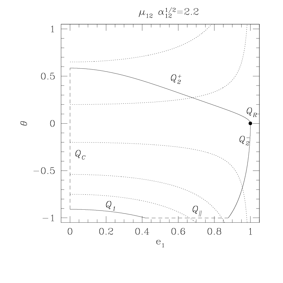
The stationary point family connects the prograde family and the retrograde family . The stationary point family connects the retrograde families and . The various families shift as a function of mass and separation, and Figure B1 of the online appendix shows a general overview of these relationships, as a function of and .
To understand the dynamics of the system near each of these points, we plot curves of constant energy, subject to the constraint of angular momentum conservation. This latter condition establishes a relationship between and , such that
| (14) |
Figure 2 shows the curves of in the case of and . In the panel in the upper right, the green curve shows the stationary point family for these parameters. The blue curve in the same diagram represents a curve of constant , chosen such that for . The main panel then shows curves of constant energy, subject to the constraint that the angular momentum has the above value. The blue contour is the one that corresponds to our chosen initial conditions, and the green contour illustrates the libration about the family. This is the standard Kozai-Lidov family and therefore the family is a stable equilibrium – a ‘fixed point’ family. This case represents the point in Figure B1.

The panel in the upper left of Figure 2 also illustrates the nature of the family. The vertical dotted lines illustrate the value we get from equation (8) for this case. Thus, the libration about the point approaches along this value and then sweeps through until it emerges at the other corresponding solution to the equation. This represents the change in angle of the blue contour as it sweeps around the origin. Thus, family is an unstable equilibrium – the saddle point at .
To understand the nature of the family, we need to move to large . Figure 3 shows the case for and . We have chosen initial conditions here to provide a very large amplitude libration about the fixed point, which actually approaches . We see that this point (the location of the family of stationary points) is a saddle point. Thus, represents a family of unstable stationary points. This also results in a qualitative change in the nature of the dynamics. At lower mass ratios (such as in Figure 2), the choice of initial conditions implies either libration or circulation. For larger masses, the presence of the family now divides the space into three parts – the libration region encloses a region of inner circulation, with an outer circulation region at large .

This figure shows two red circles. The outer corresponds to the maximum eccentricity and the interior red circle in Figure 3 represents the minimum achievable with this angular momentum constraint, and occurs at . These two limits can also be read off the blue curve in the upper right panel. The argument of periastron circulates in this case, so the minimum is not part of the stationary point family.
To understand the special family we need to go to larger initial . This is illustrated in Figure B2 of the online appendix, which shows the case for , , and . There we demonstrate that the family plays the same role as , in the high mass ratio limit where the orbits never get circular, but do approach the retrograde, coplanar limit.
So, we infer that the family plays the same role as , in the high mass ratio limit where the orbits never get circular, but do approach the retrograde, coplanar limit.
The only special case left is the point . Integrations that start close to and avoid the limit, oscillating to but , so OR is a saddle point. This is despite the fact that the stationary point intersects the continuation of the prograde and retrograde branches of the family. This saddle point is therefore the ultimate cause for why one does not get flips of the orbital plane at the quadrupolar level of approximation.
The classification of the stability of the various quadrupolar stationary points (whether solutions librate about the equilibrium – a fixed point – or avoid the equilibrium location – a saddle point) are summarized in Table 1.
3 Stationary Points at the Octopolar Level
The neatness of the quadrupolar analysis relies, in part, on the fact that does not appear in the Hamiltonian, and so we need only satisfy and . This is no longer true when the expansion is taken to octupole order, and so we must now consider, in addition, and . However, as noted by several authors (Naoz et al. 2013a; Li et al. 2014a; Antognini 2015; Naoz 2016, e.g.,), the timescale for changes in and are usually much longer than for and , so that the short-term dynamics is often regulated by a stationary point of only and . This has the consequence that the stationary point families of the octupolar problem are intimately related to those of the quadrupolar problem.
Thus, we are searching for stationary points of the system given by equations (77), (78), (73) and (74) of Naoz 2016, reprinted in appendix A, in the planetary limit. As in § 2, the stationary points can be classified in terms of particular values of and, now also, . We must also consider the quantity when classifying these equilibria. This parameter quantifies the strength of the octupole term, and we will adopt as the criterion for restricting our analysis to the octupole level. A larger value of would require extending the expansion to higher orders to achieve accuracy. (Hamers & Portegies Zwart 2016; Will 2017, e.g.,)
We will also require a naming convention to conveniently identify particular stationary point families. Those families associated with and will be designated as – because and are aligned. The apsidally anti-aligned case () will be called . Those families with will be designed as () and () respectively (because and are perpendicular in this case).
| Name | Orbit | Stability | Comments |
|---|---|---|---|
| Prograde | Saddle point | Critical inclination starts at at low masses and tends to at high | |
| Retrograde | Saddle point | Appears for , with initially, but asymptotes to at large | |
| Retrograde | Saddle point | Generalisation of quadrupolar family . Requires . Critical inclination starts | |
| at and evolves to in high mass limit. | |||
| Retrograde | Saddle point | for and decreases to at , where it is subsumed by | |
| in the circular limit. | |||
| Prograde | Fixed point | Generalisation of Quadrupolar family Q. Critical inclination is 39.23∘ for low , | |
| increasing to 65.75∘ at , where it switches apsidal alignment. | |||
| Retrograde | Fixed point | Generalisation of Quadrupolar family . Critical inclination is 140.76∘ for low , | |
| increasing to 180∘ at . For larger it does not reach . | |||
| Prograde | Fixed point | Most robust family in face of relativistic precesson. in the high mass limit. | |
| Retrograde | Fixed point | Appears when , with . Tracks - but extends to large | |
| Retrograde | Fixed point | Satisfies for . For this has a solution at , with | |
| critical angle | |||
| Retrograde | Saddle point | For , this becomes a saddle point, at . The critical angle decreases | |
| with increasing mass, tending to in the high mass limit. | |||
| Prograde | Inner Fixed point | At low masses, for and narrows for . | |
| + | Prograde | Fixed point | Generalisation of Quadrupolar family , which reaches for and |
| . In the high mass limit, . | |||
| - | Retrograde | Fixed point | Quadrupole and Octupole apsidal switches limit to |
| Prograde | Fixed point | Emerges for for . | |
| Retrograde | Fixed point | Appears when , with . Tracks - but extends to large | |
| Prograde | Saddle point | for low , but drops to 65.75∘ at . | |
| Retrograde | Fixed Point | Large but not as large as . Appears for , assuming . | |
| Retrograde | Inner Fixed point | At low masses, for and narrows for . | |
| Prograde | Saddle point | This is related to the limits of other families noted above. | |
| Prograde | Fixed point | This is generalisation of the Laplace–Lagrange solutions. | |
| Retrograde | Saddle point | Generalisation of which it closely resembles. | |
| Polar | Saddle point | In the coplanar limit, the solution is localised unless exceeds a threshold. |
3.1 Case :
If we set , then and if . The same conditions apply if . In this instance, the conditions and amount to
| (15) |
and
| (16) |
where . The upper sign on the right hand side of these two equations applies for this case (and the corresponding case where both angles are ). The lower sign in these two equations applies for the case where and (or vice versa). This is the apsidally anti-aligned case and will be treated in the next section.
The numerical solution of equations (15) and (16) yields two families of solution, which are illustrated in Figure B3 of the online appendix. The first is family , which tends towards polar orbits () for small but moves to larger as increasesi, asymptoting to . The – relation is pretty steep and so this satisfies for only a limited range of .
A second family of solutions emerges at large , designated as and also shown in Figure B3. In the limit of large this again trends towards . In the high limit, we find that this family is restricted to a finite range of . This stationary point is clearly related to the dynamics identified by Naoz et al. 2017 and de Elía et al. 2019 in the context of the outer test particle case. We will discuss this more in § 6.1.
3.2 Case : ,
This case represents the lower sign choice in equations (15) and (16). In physical terms, it means that the arguments of periastron of the two planets are apsidally misaligned by 180∘. Examples of the resulting stationary point families are shown in Figure B4 of the online appendix. Unlike for case , viable solutions only start to appear for mass ratios (for ). Formally, we can find stationary points at smaller mass ratios, but they all occur for . This implies that such points may exist but a full description may require higher order terms. For large enough , the solution extends to low and and represents the complementary case for the solutions.
The first stationary point family to appear (as we increase ) is family , which manifests in Figure B4 as a family of retrograde orbits and large , and is restricted to approximately circular orbits (). As increases, this family moves towards more inclined (but still retrograde) configurations, and with larger . For large enough mass ratios, a second family appears, which we term . This is because the properties of these stationary points bear a strong similarity to the quadrupole family discussed in § 2.1. The – relation for tracks almost exactly the equation (3) for , for the relevant masses. The value of , in this case, is small but not exactly zero.
As continues to increase, the two branches merge into a single continuous family, bounded from below by a minimum . For , the part of the curve is restricted to a narrow range of , in a similar fashion to family of § 3.1. The curve also extends to lower , but there appears to be a gap. We will discuss this further in § 6.1.
3.3 Case :
The third case occurs when both arguments of periastron are at right angles with respect to the line of nodes. Once again, this choice of parameters automatically satisfies and , leaving the following conditions to locate the stationary points
| (17) |
and
| (18) |
As in the previous sections, the upper sign in equations (17) and (18) refers to the case of apsidal alignment, while the lower sign represents the anti-aligned case (, ).
Figure 4 shows the different solutions in case , as a function of mass. Once again, all solutions are shown for . In red, we show the solutions for (lower mass ratios are qualitatively similar). Most obvious is a family of solutions that corresponds closely to the quadrupolar family – the Kozai-Lidov family. As in the quadrupolar case, this family becomes increasingly asymmetric with increasing and so we refer separately to (prograde case) and (retrograde case). As in the case of , this family is found with small, but finite, .
As the mass ratio increases, we also see the appearance of a second family, which we term . Examining the blue curves in Figure 4, we see that the family appears to track quite closely in terms of –, but deviates strongly in the upper panel, where it shows solutions with a much larger . We see also that the family has a maximum , which is also the point at which this low family merges into the higher family . We see also that the maximum value decreases as increases.

The retrograde family, also exhibits a higher counterpart which we term family , as can be seen in Figure 4. This forms initially for small and moves to larger as increases. Once again we see that the quadrupolar analogue solution merges smoothly with the higher eccentricity family.
Finally, we also find a fourth family, a retrograde family we call . Both and emerge as the lower limit of family moves away from the circular orbits.
3.4 Case : ,
Case refers to the same equations (17) and (18), but with the lower sign on the right hand side of each (positive and negative, respectfully). The stationary point families are shown in Figure 5. As one might expect, there is a fair amount of symmetry between the solutions in Figure 5 and those in Figure 4.

Perhaps the first point to note is the complementarity between these solutions and the corresponding apsidally aligned ones in Figure 4. Family + appears to be the complement of + – occurring for those values of and where the solution is not found in case . Together, they appear to comprise the full analogue of the solution. There does not seem to be an equivalent -, but that is not surprising given that appears to cover the full range of eccentricities. In § 6.1 we will show that the - family does exist, but covers only a very limited range of parameters.
We also find analogues of the high extensions of the quadrupolar analogue families in and – the equivalents of and . In addition, there exists a family , an analogue to , but this time it occurs for prograde, rather than retrograde, configurations. For large enough masses (), the families +, and form a continuous curve.
Finally, the right hand panels of Figure 5 show a family, of almost radial orbits. Superficially, these look like the mirror image of at low masses. However, as increases, does not extend along , but eventually retreats towards the radial limit again. Mass ratios of –5 (for ) mark the maximum extension of this family to smaller (which remains well above 0.9 at all times). This family is also distinct from the family in the limit of , because it is found with demonstrably less than unity (although still large). This family is characterised by large values in both the quadrupolar and octupolar terms in , which offset each other. The limited range of applicability in is a consequence of the cutoff – this family extends over a much larger range of masses if we relax this criterion.
3.5 Special Cases: Octupole limit
In the quadrupole limit, we also found that we could satisfy and in special limiting cases, where was not restricted to the same values as in other stationary point families. With the introduction of the octupole term, these families become even more restrictive, because the vanishing of this term imposes conditions beyond those imposed by the quadrupole term. We will denote the special case octupolar families with .
3.5.1 Circular Limit:
In the case of the circular limit (see § 2.3), the octupole level introduces a term , so this will only be zeroed if the coefficient of this term goes to zero simultaneously. This imposes a relationship between , and , as a function of , and . The condition reduces to the quadrupolar limit in this case.
In the low mass ratio limit, this leads to , , and (i.e. ). In the high mass limit, this requires and one of , or . These are the critical inclinations identified by (Jefferys & Moser 1966; Krasinsky 1972).
3.5.2 Coplanar Limit: and .
In the quadrupolar limit, we also found family (see § 2.5) in the limit of coplanar, retrograde orbits. So, let us now examine the case of . In this case, we find that and are satisfied by the condition . In the prograde case (), this relation can be maintained by , because the equation derived from this condition is
| (19) |
which depends only on the angle . This is the extension of the traditional Laplace-Lagrange treatment (e.g. Murray & Dermott 1999) to the hierarchical case (Lee & Peale 2003; Michtchenko & Malhotra 2004, e.g.). As in the traditional case, this yields two solutions corresponding to or , although the nonlinearity of the system means that these no longer form a basis set for describing more general behaviour. Figure 6 shows an example solution. Both curves asymptote to a fixed value of at small eccentricities, which matches the expectations from the traditional expansion. We will refer to this family as ’’, since it represents the extension of the Laplace-Lagrange family. Note that this analogue of the classical family appears first at octupole order, since it depends on the difference between and .

In the retrograde case, the equation for depends on , and so it is only a stationary point if as well. This implies also, i.e. the same fixed point condition as in the other cases. From this we derive a relationship between and that is an extended version of equation (9) which yields a qualitatively similar solution – we find sensible solutions only in the retrograde case and for sufficiently large . In the online appendix,Figure B10 shows an example of the solution for the case and . The shape of the solution closely tracks the quadrupolar version, but there is a change of apsidal alignment along the curve. Comparison with the other solutions shows that this family forms the same kind of link between and as the corresponding quadrupolar solution does. We will call this family .
3.5.3 Radial limit:
Finally, we have the radial limit . In this limit, automatically, and imposes additional constraints, given by the condition
| (20) |
This is automatically satisfied if or but more general combinations of , and also satisfy this criterion. The addition of the constraint that as well does not restrict the solutions because in this limit. This leads to a rather broad family of possible solutions, which we term .
An important potential application of this family is in the case of coplanar orbits (). In that instance, the more general class of solutions are clustered near or , unless is above some threshold value. We can estimate the critical by setting and deriving the resulting from
| (21) |
The requirement that imposes a condition on . For , this is . Figure 7 shows the nature of the solution near this critical value. We see that the shift is quite dramatic, over only . Note that the form of equation (21) is the same as the expansion parameter , so that the critical value can also be expressed as a critical . This becomes relevant in the case of coplanar orbital flips, as discussed in § 6.3.

4 Effect of Relativity
For planets in short period orbits, the effect of relativistic precession must be included. The addition of a component of from relativity can shift the location of these stationary points. Indeed, relativistic effects can give rise to qualitatively new features in the case of massive outer perturbers or comparable mass inner binaries (Naoz et al. 2013b; Naoz et al. 2017; Naoz et al. 2020; Will 2014; Will 2017; Liu et al. 2015; Liu et al. 2019; Lim & Rodriguez 2020, e.g.,), but, with our focus on the planetary case, we will limit our attention to the post-Newtonian correction to the inner orbit precession.
Relativistic precession is usually discussed in the context of the suppression or excitation of orbital eccentricity, but it can shift both the inclination and eccentricity of the stationary points (Migaszewski & Goździewski 2011, e.g.). To illustrate this, let us consider the addition of a relativistic contribution (equation 57 of Naoz 2016) to the right hand side of equation (2). If we set in the case of (the solution), we now derive a modified condition on the inclination of the fixed point, namely
| (22) |
where and
| (23) |
and , are the semi-major axes of the inner and outer planets, and is the Schwarzschild radius of the central object. This is essentially a ‘squashed’ version of the original family, since e1 is now bounded from above at a smaller value than unity. The equivalent correction for the family shifts the mass threshold at which it appears. Note also that the relativistic contribution has broken the scale invariance of the problem, since lengths are now scaled relative to .
Figure 8 shows the effect of relativity on the fixed point families of the full octupole problem, as we move the system closer to the star, while keeping fixed. The upper two panels show the case of (realised in this case by and ). Far from the star, the fixed point families should look as they do in Figure 4 and 5. However, the upper panel shows that, if AU, then the effects of relativity are significant. The quadrupolar family is squashed and distorted, and the positions of additional families (such as or ) are shifted as well. The middle panel shows the effect of moving the system in even further (AU). We see now that the and families no longer intersect the quadrupolar family (which is now squashed down to e1<0.2).

The bottom panel of Figure 8 shows what happens if we decrease the mass ratio to (M) at this location. Now the quadrupolar family has completely disappeared (Ford et al. 2000; Naoz et al. 2013b; Naoz et al. 2020, see also), but the and families remain. This illustrates that the inner planet mass is important too.

One of the reasons to be interested in the effect of relativity is in the case of planet migration driven by secular interactions and tides. In this case, we should keep the outer planet location fixed ( fixed, rather than ) and move inwards. Thus, as decreases, for fixed , the contribution increases more rapidly. When the numerator factor in equation (22) equals zero, and this is the maximum for which the quadrupolar solution remains, namely
| (24) |
Eventually, is small enough that , which yields the criterion for the Kozai-Lidov family to survive:
| (25) |
Figure 9 shows the evolution of the full fixed point family (to octupolar order) in an example where we hold the outer perturber fixed at 20 AU, but move the inner planet closer to the star. We show here the stationary point families in the case of . We see the evolution of this ‘squashed’ Kozai-Lidov family to ever smaller as decreases. However, we see that the family remains and plays an ever larger role as decreases. This family starts at and extends up to almost radial orbits. The family is also strongly polar. Even when the family disappears, the family continues to exist for non-zero e2. This eventually disappears too at AU (for this example). The equivalent anti-aligned case () shows a similar form but extends to slightly retrograde orbits instead of slightly prograde ones.
The cases remain qualitatively similar with the introduction of relativity. Of more interest are the special cases, because the allowed values of are shifted by the relativistic precession, and because tidal circularisation naturally takes us to the limit. The one that survives the furthest in is the polar limit, wherein
| (26) |
For this to provide a physically reasonable answer, , which implies
| (27) |
Comparison with equation (25) shows that the saddle point survives longer than the Kozai-Lidov quadrupolar fixed point family as a planet is dragged down by tides.
Thus, the effects of relativity start to have a marked effect on the stationary point families for AU. In the case where we keep fixed – so that decreases as does, the bulk of the stationary points are wiped out by AU. For more compact systems, wherein we keep fixed as we move the planet pair inwards, some stationary points can survive interior to 0.1 AU. A generic tendency is for the surviving stationary point families to lie close to polar.
5 Stability of the Stationary Point families
In the previous sections, we reviewed the stationary point solutions of the octupolar-level expansion of the hierarchical three-body problem. This identifies equilibria, but does not specify the stability of said equilibria. Here we shall review each family of stationary points in order to determine their stability – whether they are fixed points or saddle points – and their role in fixing the orbital structure. Furthermore, we will do this as a function of . In the previous section we arranged our solutions in terms of their apsidal alignment, but it is also instructive to see how the various classes fit together for particular mass ratios. We will once again fix , so that we can vary alone. The results are summarised in Table 2.
To determine stability, we will make use of the fact that the short-term dynamics are still driven primarily by the quadrupolar term (Naoz et al. 2013a; Li et al. 2014a; Antognini 2015; Naoz 2016), with longer-term drifts imposed by octupolar contributions. So, we first construct contours of constant energy and angular momentum, to identify whether the underlying short-term dynamics are consistent with a fixed point or a saddle point. We then follow this with direct integrations of the full octupolar equations to verify whether the octupolar terms change the long-term dynamics.
In the octupolar case, we also encounter families where librates about the equilibrium while displays a saddle point behaviour. In this case circulates, but can show a brief reversal that qualifies as a solution to our equilibrium conditions of . In this case we will refer to an ‘inner fixed point’.
5.1 Low mass ratios:
Empirically, this is the most common kind of system observed in exoplanet systems. It is also the least complicated case, because the small inner mass induces a limited precession of the outer mass and so the configuration of the stationary point families hews pretty close to the quadrupolar case. Figure B5 of the online appendix summarises the stationary point families present.
5.1.1 Kozai-Lidov Analogue:
As one might expect, this limit is dominated by the and families, the generalisation of the Kozai-Lidov family. However, despite the low , both and librate so these represent a full generalisation of the Q2 families to the octupolar case. Figure B6 of the appendix shows an example of such a trajectory.
5.1.2 Saddle Points:
The family is also present in the low limit, where it occurs for almost polar orbits. This is a saddle point. A trajectory that begins near this point exhibits large-scale variations in , and is located at the extreme of librations about the fixed point. This stationary point performs the same role as the fixed point in the quadrupole description (see § 2.3 and Figure 1), but is more localised because it includes the criterion that , which restricts the family to almost polar configurations. It is also worth noting that many of these trajectories yield intermittent orbital flips, as can fluctuate about the polar value.
5.1.3 Radial Families
One feature to note, in addition to the analogues of the quadrupolar families, is the presence of the quasi-radial stationary point families , and , as shown in Figure 10. To demonstrate their role, we choose a starting point close to , and integrate the equations for different initial apsidal misalignments (varying keeping fixed). Although the curves pass through the same point in – space, these equilibria exist for large as well. The examples shown in Figure 10 are integrated using an initial .
These integrations establish that (red points) and (blue points) are examples of the inner fixed point variety discussed above – the angle does not librate over a finite range but circulates, while librates. The circulation of introduces a small variation in the parameters that can generate orbital flips if the librations are large enough to approach or . However, this requires large amplitude librations – we have not found cases where the small amplitude librations are destabilised, because the variation in is not large for low . If we start with enough apsidal misalignment, we do indeed see orbital flips, as shown by the cyan points. These integrations also establish the relationship between the different radial families. The and families are inner fixed points and the family is a saddle point that separates the regimes of libration and circulation of , as shown by the green and black points.

5.2 Comparable mass ratios:
As the mass ratio becomes comparable, the effects of the inner planet on the outer become stronger, and start to introduce features not found in the limit of an inner test particle. Figure 11 shows the different stationary point families for the case . The four different cases for and are shown in blue (Case ), cyan (Case ), red (Case ) and black (Case ).
5.2.1 Kozai-Lidov Generalisations: and
We see that the most prominent feature is still the generalised version of the Kozai-Lidov family ( and ). We see also the emergence of the family, the eccentric version of the K-L family.


Figure 12 shows the contours of constant energy for the case where the angular momentum is given by the upper dotted line in Figure 11. We also need to specify a value of , because this contour crosses both the and families, which have very different values of at their intersections. We know that the family is a stable point from the quadrupolar analysis, so we choose to isolate the stationary point. From the contours in Figure 12 we identify as a stable equilibrium – a fixed point. We confirm this by a direct integration of the orbital equations, shown in red. The finite width of the libration trajectory is a consequence of the small variation of (which is assumed to be constant in the calculation of the contours). Therefore, represents a high eccentricity offshoot of the family.
5.2.2 The Prograde Saddle Points: and
The families and exist at low (for all and ). Direct integrations from the starting points of and families indicate that these two are saddle points, representing the minima of large amplitude librations or circulations. These saddle points are also associated with the special case solutions . The dotted lines in Figure 12 indicate the angle appropriate for the special case – it is along this angle that large amplitude librations approach the saddle point at the origin. The geometry of the curves in this figure also illustrate the nature of the and stationary points – the curves that turn away from the origin indicate that these are saddle points. Inspection of Figure 12 might suggest that saddle points exist for all four possible apsidal alignments, but the requirement restricts this to just the and cases.
5.2.3 The Retrograde Families and
At the lower left in Figure 11, the cyan feature represents the appearance of the and retrograde orbital families. The family appears to be a high eccentricity offshoot of the traditional Kozai-Lidov quadrupolar family, but the families and appear to be qualitatively distinct. Figure 13 shows two examples of direct integration - one chosen from the branch and one from the branch. The family is shown to be a stable fixed point family, with both and librating about the equilibrium values. The family, on the other hand, shows libration of on short timescales, but an overall circulation of the libration centre on longer timescales, combined with circulation of . We find that the combination librates about a value of in this case, which means that the two planets precess at roughly the same rate and maintain a maximal separation of their perihelia. The value of also undergoes a large excursion with a minimum at the stationary point, so the family is most accurately characterised as a saddle point. These two families are likely to be related to the known families of stable retrograde orbits in the problem of equal masses (e.g. Henon 1976).

5.2.4 The Laplace–Lagrange Analogues:
For completeness, we note also the presence of the two families in this case, but do not discuss them further as their behaviour and stability is well documented (Lee & Peale 2003; Michtchenko & Malhotra 2004) – at least until they approach the orbit crossing limit.
5.3 Large mass ratios:
The landscape of stationary points gets more complicated as the mass ratio increases – as is shown in Figure 14. This is not surprising, as a more massive inner planet is more capable of affecting the orbital dynamics of the outer planet.

5.3.1 The Kozai-Lidov generalisations: , and : , and
The asymmetry of the Kozai-Lidov family between prograde and retrograde is clearly evident in Figure 14. More interesting is the fact that the prograde branch is split into an apsidally aligned () and apsidally anti-aligned () branch. Both also merge smoothly into their higher analogues and . The family now also merges smoothly with the family. The retrograde family now shows a high eccentricity offshoot as well, with and now present at large .
Figure B7 of the online appendix shows the energy contours along the two uppermost of the dotted lines in Figure 14, representing two choices for the total angular momentum of the system and illustrates that the and families still represent stable librations, as they did for lower mass ratios.
Figure 15 shows the orbital behaviour near the and families of retrograde orbits in the bottom right of Figure 14. We see that these correspond to a fixed point, i.e. a stable equilibrium. This is therefore the high equivalent of , just as and are the high equivalents of the family.

This new set of families first appears at when the family passes through and . This is also the point at which the special family appears, with , and so this becomes degenerate with the family. We see no equivalent split on the prograde side because would require a much larger and the family does not pass through any such point. A more general criterion for the appearance of this family can be obtained by noting that the family represents the limit of the / families.
5.3.2 The Saddle Points: , , , and
Also apparent in Figure B7 is that there is a saddle point close to the origin – these are the and stationary point families that are also present at lower masses. The families and were also present at lower masses, but were found at retrograde inclinations and moderate . They have now shifted to an inclined family or almost circular orbits, and are now saddle points. In the case of this is a change in the behaviour of this family, relative to the discussion in § 5.2.3.
Figure 16 shows the evolution of e1 versus in examples from the family for four different mass ratios – from the last section, from this section, and two intermediate values and . We see that the transition occurs between and 3, and results when the family switches from a retrograde family at small , to a circular family slightly inclined relative to retrograde coplanar. Thus, increasing destabilizes the family, turning it from a fixed point to a saddle point. This is a consequence of the increased libration and eventually circulation of , which causes to circulate, with only intermittent libration.

The family also retains its saddle point nature, as expected (since is small along this family). This is shown in Figure B8 of the online appendix, which shows both the point at , but also the fixed point at . Unlike the prior contour plots, this one does not allow solutions for the full range of , because the dotted curve corresponding to the fixed angular momentum does not extend to in Figure 14.
5.4 Extreme Mass ratios: and
Figure 17 shows the evolution of the stationary point families as continues to get larger and starts to approach the outer test particle limit. The behaviour of the stationary point families can be divided into several subsets.
5.4.1 The Kozai-Lidov Generations: , , ; and
As shown in Figure 17, at , the prograde families and are compressed to and they disappear completely by (although vestigial versions of , and remain). The family comes to dominate at these masses, and becomes progressively more polar as the mass ratio increases.
5.4.2 The Saddle Points: , , and
Similarly to , the family evolves towards the polar limit as increases, but from the retrograde direction.

At larger , the family moves to larger and truncates when it intersects . Furthermore, we finally see the appearance of the family discussed in § 3.1. We see that it is also clearly associated with the / family, filling in a gap in the family at . The appearance of the family produces a new saddle point. This has qualitative similarities to the point, as it divides the parameter space into an inner and outer region of circulation, which encircle a libration (about the fixed point). This is demonstrated in Figure B8 of the online appendix.
The family merges smoothly into the saddle point family , so one question, based on Figure 17 is whether, in the limit of large , the prograde solutions are entirely of family , or whether a family of saddle points remains. Examination of the black curve for shows that this entire curve is stable – i.e. belongs to the family. Thus, disappears at the same time as .
5.5 Influence of Relativity
In § 4 we showed that the inclusion of relativistic precession alters the positions of the stationary point solutions if the inner planet orbits too close to the star. It also has consequences for the stability of those equilibria.
In particular, the inclusion of relativistic precession appears to destabilise both the quadrupolar extensions as well as the and families seen in the panels of Figure 8. An example of this is shown in Figure 18. We see that does librate intermittently, but also experiences circulation and fluctuations in , which are driven by the circulation of the angle . Thus, we cannot regard this family as a fixed point family anymore.

The family that does remain stable is , in which both and librate for starting conditions taken from all three panels in Figure 8. The corresponding family in the lower panel shows libration of but circulation of , which introduces a larger amount of variation in .
This prograde, polar fixed point family is stable even when the quadrupolar family is destroyed by the relativistic precession, and extends down to at least AU in the case where and . Of perhaps greater relevance is the case where the inner mass and semi-major axis is fixed and the outer values varied, as this is more representative of the observational situation. The sequence shown in Figure 9 is more representative of this, and shows that the family persists in this sequence as well. It also remains stable as and/or increases. However, it does move to ever higher , although remains below the threshold level of 0.1 because is also dropping.
5.6 Influence of Orbital Separation
We have so far focussed on the mass ratio, , as the principal parameter, holding the ratio of separations fixed at . At the quadrupolar level, the stationary point structure is regulated by the quantity , so that the configurations for smaller should largely mimic those at but with lower . At the octupole level, an additional consideration is the fact that changing will change the value of corresponding to the threshold . A comparison at fixed but different is shown in Figure B11 of the online appendix. As expected, shifting from to moves the families towards a configuration more reminiscent of the lower mass case in Figure B5. Similarly, moving to larger shifts the configuration more towards that observed in Figure 17.
If gets too large, the neglect of higher order terms becomes problematic and the hierarchical assumption fails. However, at least some of the stationary points discussed here appear to survive at closer separations. Studies of the secular structure of specific exoplanet pairs by direct numerical averaging of the secular hamiltonian (Michtchenko et al. 2006; Migaszewski & Goździewski 2009) show fixed points associated with Kozai-Lidov resonances as well as several additional families. Section § B4 of the online appendix discusses the relationship between the naming convention used here and that used in Migaszewski & Goździewski 2009; Migaszewski & Goździewski 2011. These studies focus either on a limited mass range and more compact configurations (Migaszewski & Goździewski 2009) or high masses but only prograde orbits (Migaszewski & Goździewski 2011), but indicate that the structure we discuss here is robust beyond the hierarachical approximation.
6 Discussion
Table 2 summarises the different stationary point families and clarifies which are fixed points and which are saddle points. In terms of stable stationary points (fixed points), we find that the octupole problem shows analogues of the quadrupolar Kozai-Lidov family (, ) for low but finite as well as branches that exist at large ( and ). We also find that these branches switch apsidal alignments in certain places, driven by the direction of the precession of at quadrupole order. We find a branch of fixed points at almost radial orbits ( and ) and another stable family of fixed points in a retrograde configuration ( and ). The stationary point structure is much richer for than it is for .
An analogue of the saddle point also appears at large , in the form of , and , with branches for both small and large in a manner similar to the / family fixed points. The set of saddle point families , , and define the seperatrices of large scale librations about the and fixed point families in the limit . There are also generalisations of the special case saddle points for circular, radial and coplanar orbits.
6.1 Switching of Apsidal alignments
One curious feature of the solutions to the octupole problem is that, although extensions of the quadrupolar families are present, the generalised families switch apsidal alignment for particular values of . This can be understood by noting that the sign of the octupolar contribution must change whenever the sign of the quadrupolar contribution switches sign, in order to fix the stationary point. Thus, we can identify the switches in apsidal alignment by finding the cases when at quadrupole order.
At low there are no switches in apsidal alignment. As we increase , the first case arises in the limit . If we take the limits of the prograde versions of equations (4) and (11), we find the critical value at which this apsidal switch first appears from the requirement that the two expressions have the same limit, namely
| (28) |
This is satisfied when . Therefore, the two curves first overlap when for . For mass ratios above this value, the prograde analogue of the solution is split between + and +, with the transition moving to lower as increases.
As the mass ratio increases, the point of reversal moves to lower and eventually disappears again. The corresponding mass can be derived from the limit, which yields , or for .
Similar behaviour occurs for the retrograde branches. In this case, the alignment reversal sets in at lower masses in the limit. There is no closed form solution for this criterion, but numerically it is . As the mass increases, the reversal moves to larger , with a limiting behaviour in the large limit of
| (29) |
The retrograde solutions exhibit another curious feature, in that the octupolar contribution to contains a term . The - and - solutions occur in the limit of low so fixing a stationary point in this limit requires that the coefficient of that term must go to zero too, which imposes a condition as well. When the solutions cross this threshold, there is another apsidal reversal. The consequence is that the - contribution is limited to a finite range of and . The inset in Figure 19 illustrates this.

Related behaviour is apparent in the solutions. At the quadrupolar level, yields equation (13). Reversals in apsidal alignment are therefore to be expected when this criterion overlaps with the criterion, which leads to the condition
| (30) |
The lowest mass for which a solution occurs is found by setting , and so we expect apsidal reversals when , which amounts to for . We note also that solutions are limited to because otherwise . The approach to this limit leads to large , which explains why this eccentricity was identified as a critical value for the outer test particle case (Naoz et al. 2017; Zanardi et al. 2017; Zanardi et al. 2018; Vinson & Chiang 2018; de Elía et al. 2019; Naoz et al. 2020).
As in the case of the and families, we see that the apsidal reversal between and families also only occupies a limited range of , and for the same reason. The criterion that the octupolar term be finite as for this case implies a condition . In the limit of very large masses, and . Together these eccentricity limits explain the behaviour of the retrograde families in Figure 17.
6.2 The Eccentric Kozai-Lidov Mechanism
One motivation for this work was to get a more unified view of the rich dynamical structure (Naoz 2016, e.g.) of the hierarchical three body problem, using the stationary point families as a ‘scaffolding’, or organising principle. The most obvious feature of the dynamics of this problem is the Kozai-Lidov resonance (Kozai 1962; Lidov 1962), which couples the eccentricity and inclination variations due to a resonance between the apsidal and nodal precession rates. The original (quadrupole) description of this resonance is associated with our family of fixed points, although the saddle point is also important, as it represents the turning point of the librations about the family.
The appreciation that the octupolar contribution can qualitatively change the dynamics (Naoz et al. 2011; Naoz et al. 2013a) motivates the generalisation of the study of the stationary points to the more general octupolar case. We see that the form of the K-L fixed point family retains its basic nature with the introduction of the octupole term, although we note that the apsidal alignment between inner and outer orbits does vary depending on the eccentricity and mass ratio.
Figure 20 shows the evolution of a system with the same parameters as those shown in Figure 6 of Naoz et al. 2013a – a demonstration of the kind of orbit orientation flip introduced by the inclusion of the octupole term in the dynamics. The evolution of the system is plotted relative to the particular stationary points relevant to the dynamics of this particular case. We see that the fundamental libration is still driven by the location of the family, but the turnaround at low e1 is associated with the saddle point. It is also notable that the range of over which the value of e1 remains low is regulated by two of the solutions of the special family – depending on the value of the mutual inclination. The excursions at large e1 do come close to the special point, but are regulated by the limited variation allowed by the conservation of angular momentum (even including the variations induced by libration of e2).

The generalisation of the K-L family – – occurs for small, but non-zero . We do find, however, that there are extensions of this fixed point family to high (the / and /) families. In particular, the and families share very similar trends in terms of e1 and , but differ dramatically in terms of e2. Are they truly distinct?
Figure 21 shows the results of three integrations that all start from the same initial conditions except for a different value for e2. The masses are , and , while the semi-major axes are AU and AU (so ). The inner eccentricity is and . We also assume . For these values, the fixed point is located at and the fixed point is located at . The figure shows the evolution for e2=0.03 (black), 0.4 (blue), and 0.77 (red).

For low values of e2, librates, as expected for the +fixed point. However, for in the range 0.1–0.7, circulates, although continues to librate. This is consistent with the behaviour expected of a generalization of the quadrupole behaviour, since plays little role in the evolution of if the octupolar contribution is weak. However, Figure 21 shows that libration of returns at . This is the appearance of the fixed point. Thus, the point is qualitatively distinct from the point in the sense that we find an extended range of e2 in between the two fixed point values, for which circulates.
6.3 Coplanar Flip Behaviour
Li et al. 2014a noted the appearance of an orbital ‘flip’ behaviour in systems with almost coplanar orbits but high eccentricities. This is qualitatively different from that associated with the Kozai-Lidov family in that it starts from approximately coplanar configurations and also transitions from prograde to retrograde on a timescale considerably shorter than the diffusive evolution seen in manifestations of the Eccentric Kozai-Lidov effect.
This appears to be related to the radial fixed point family discussed in § 3.5. Li et al discussed the case of and find that the orbit flips if the outer body eccentricity is large enough. The family is a saddle point, and so the approach to this limit in the coplanar case drives the system away from the equilibrium. As noted in § 3.5.3, the range of for which the equilibrium exists is limited unless e2 is large enough. If we apply our criterion equation (21) for the critical solution to extend over all , we derive a criterion , which compares well to Li et al’s empirical estimates for the threshold value. They also find a restriction to large initial , but this is more related to the initial conditions – it is required to limit the value of the z-component of the angular momentum to a value that is less than the variation induced by the octupolar term.

Figure 22 shows an integration of the case chosen by Li et al. 2014a in Figure 2 of that paper. We see that the ‘flip’ is indeed associated with a saddle point in – where the direction of precession reverses. For lower values of e2, the precession of does not reverse and the inclination increases by only a small amount. We also highlight the cycle in that leads to the flip in blue. This demonstrates the speed at which the transition occurs – because it is a direct passage through the saddle point and not a diffusive evolution like in the case of the flips driven by the Eccentric Kozai-Lidov evolition.
6.4 The Inverse Kozai-Lidov Resonance
The original Kozai-Lidov solution represents the fixed point associated with an inner test particle, and is found above a critical inclination (at low ) of . The equivalent solution for an outer test particle yields another critical inclination at (Jefferys & Moser 1966; Krasinsky 1972; Lidov & Ziglin 1976) at quadrupole order. Figure 23 shows the critical inclinations (the limit) of various orbital families, as a function of (keeping ). The changeover from the family to the contribution is because and have different quadrupolar limits as the mass ratio increases, and it requires large octupolar corrections to satisfy both criteria simultaneously. Eventually this violates the criterion, although the addition of higher order terms can recover a solution in this limit (Gallardo et al. 2012; Naoz et al. 2017; Vinson & Chiang 2018; de Elía et al. 2019).

Within context of our classification, the ‘inverse Kozai-Lidov resonance’ (as defined by Vinson & Chiang 2018) is related to the high- extensions of the original quadrupolar family ( for the prograde case, for the retrograde case) rather than the low extensions and that form the natural generalisations of the Kozai-Lidov family, as these latter families either tend to polar or disappear in the high limit.
6.5 Warm Jupiters
The presence of giant planets on scales –1 AU (‘Warm’ Jupiters) is considered to be a curious phenomenon, given that the most common theories of giant planet formation suggest that planets are easier to form on larger scales. The presence of ‘Hot’ Jupiters, with AU is suggested to be a consequence of either migration through a disk to the inner edge (Goldreich & Tremaine 1980; Lin & Papaloizou 1986; Lin et al. 1996) or by the tidal capture of planets excited to high eccentricity orbits due to either planetary scattering (Rasio & Ford 1996; Weidenschilling & Marzari 1996) or secular interactions (Fabrycky & Tremaine 2007; Naoz et al. 2011; Wu & Lithwick 2011; Naoz et al. 2012; Stephan et al. 2018, e.g.,). Warm Jupiters fall in between these two classes. It has been proposed that such planets may be in the process of a slow or stalled tidal drag-down because their periastra get close enough to the star for meaningful tidal dissipation only for a small fraction of the duration of secular oscillations (Dong et al. 2014; Petrovich & Tremaine 2016; Frewen & Hansen 2016). Dawson & Chiang 2014 present evidence that Warm Jupiters with outer planetary companions have substantial mutual inclinations, based on the clustering of the projected near values . This clustering is related to the fact that systems undergoing large librations about the family approach the saddle point and the preferred value of emerges from the location of the family in the limit of (which holds for most of the Warm Jupiter systems).
6.6 High Eccentricity Orbits
Much of the interest in hierarchical triples derives from their potential to generate high eccentric orbits through Kozai-Lidov oscillations (Naoz 2016). One new feature identified here is the existence of highly eccentric fixed point families, where the eccentricity remains high. The and families exist for approximately polar orbits, while the and families exist for retrograde orbits in the limit of large . These families of orbits potentially offer alternative pathways to high eccentricity migration, but would require a dissipative process to place a system into such a configuration if one started from a traditional coplanar alignment.
7 Conclusions
Our goal in this paper is to survey the stationary points of the hierarchical three body problem. We aim to understand the variety of possible secular behaviours available to planetary systems in hierarchical configurations.
The principal feature at the quadrupole level of approximation is the fixed point family , identified originally by Lidov and Kozai (Kozai 1962; Lidov 1962), along with several saddle points that appear in various limits (Ziglin 1975; Lidov & Ziglin 1976). We find that the same fixed point behaviour appears at the octupolar level, for small but non-zero values of the outer planet eccentricity e2, although it is split between two fixed point families, and , depending on whether and are aligned or anti-aligned. An interesting feature of these families is that, for larger mass ratios, the apsidal alignment can change as a function of . These switches are associated with the change in sign of and at quadrupole order.
In addition to identifying the analogue to the quadrupolar family, we also identify extensions to this family, with both prograde and retrograde cases. These new fixed point families are distinct in that they are branches that continue up to much larger and have no analogue at the quadrupolar level. They demonstrate that the octupolar contribution can do more than simply induce variations about the quadrupole solution and contribute to chaos – it can also help to fix and stabilise new equilibria. Elements of these families are also the most robust against the destabilising effects of relativistic precession when the inner planet gets close to the central star.
The secular architecture gets more diverse as increases (at fixed ), with the various new fixed points appearing for and the original Kozai-Lidov family tending to polar orbits as gets large. We also find several stationary points for retrograde configurations.
We also find a variety of special case solutions, most of which are saddle points (although we recover the known extension of the Laplace-Lagrange solution in the coplanar limit). As one would expect, many of these are associated with the transitions between circulation and libration about one of the fixed points. One saddle point of dynamical significance is that in the radial, coplanar limit, which is responsible for the coplanar flip behaviour identified by Li et al. 2014a.
These results indicate that the secular architecture of multiplanet systems contains several possible fixed points, especially in the case of more massive inner planets. Although current methods of planet detection yield only weak constraints on mutual inclination in most cases, the anticipated astrometric information to be gained from GAIA in the near future (Perryman et al. 2014) may allow us to constrain the full three dimensional behaviour of the best studied systems and to classify their dynamics in terms of the behaviour outlined here.
This research has made use of NASA’s Astrophysics Data System and of the NASA Exoplanet Archive, which is operated by the California Institute of Technology, under contract with the National Aeronautics and Space Administration under the Exoplanet Exploration Program. S.N. acknowledge partial support from the NSF through grant No. AST- 1739160. Moreover, S.N. thanks Howard and Astrid Preston for their generous support. The authors acknowledge a helpful referee report.
Data availability: All data used in this paper are available upon request from the corresponding author.
References
- Antognini (2015) Antognini J. M. O., 2015, MNRAS, 452, 3610
- Dawson & Chiang (2014) Dawson R. I., Chiang E., 2014, Science, 346, 212
- Dawson & Johnson (2018) Dawson R. I., Johnson J. A., 2018, ARA&A, 56, 175
- Dong et al. (2014) Dong S., Katz B., Socrates A., 2014, ApJ, 781, L5
- Fabrycky & Tremaine (2007) Fabrycky D., Tremaine S., 2007, ApJ, 669, 1298
- Ferrer & Osacar (1994) Ferrer S., Osacar C., 1994, Celestial Mechanics and Dynamical Astronomy, 58, 245
- Ford et al. (2000) Ford E. B., Kozinsky B., Rasio F. A., 2000, ApJ, 535, 385
- Frewen & Hansen (2016) Frewen S. F. N., Hansen B. M. S., 2016, MNRAS, 455, 1538
- Gallardo et al. (2012) Gallardo T., Hugo G., Pais P., 2012, Icarus, 220, 392
- Goldreich & Tremaine (1980) Goldreich P., Tremaine S., 1980, ApJ, 241, 425
- Hamers & Portegies Zwart (2016) Hamers A. S., Portegies Zwart S. F., 2016, MNRAS, 459, 2827
- Harrington (1968) Harrington R. S., 1968, AJ, 73, 190
- Henon (1976) Henon M., 1976, Celestial Mechanics, 13, 267
- Innanen et al. (1997) Innanen K. A., Zheng J. Q., Mikkola S., Valtonen M. J., 1997, AJ, 113, 1915
- Jefferys & Moser (1966) Jefferys W. H., Moser J., 1966, AJ, 71, 568
- Kozai (1962) Kozai Y., 1962, AJ, 67, 591
- Krasinsky (1972) Krasinsky G. A., 1972, Celestial Mechanics, 6, 60
- Lee & Peale (2003) Lee M. H., Peale S. J., 2003, ApJ, 592, 1201
- Li et al. (2014a) Li G., Naoz S., Kocsis B., Loeb A., 2014a, ApJ, 785, 116
- Li et al. (2014b) Li G., Naoz S., Holman M., Loeb A., 2014b, ApJ, 791, 86
- Libert & Henrard (2006) Libert A.-S., Henrard J., 2006, Icarus, 183, 186
- Libert & Henrard (2007) Libert A.-S., Henrard J., 2007, Icarus, 191, 469
- Libert & Tsiganis (2009) Libert A. S., Tsiganis K., 2009, A&A, 493, 677
- Lidov (1962) Lidov M. L., 1962, Planet. Space Sci., 9, 719
- Lidov & Ziglin (1976) Lidov M. L., Ziglin S. L., 1976, Celestial Mechanics, 13, 471
- Lim & Rodriguez (2020) Lim H., Rodriguez C. L., 2020, arXiv e-prints, p. arXiv:2001.03654
- Lin & Papaloizou (1986) Lin D. N. C., Papaloizou J., 1986, ApJ, 309, 846
- Lin et al. (1996) Lin D. N. C., Bodenheimer P., Richardson D. C., 1996, Nature, 380, 606
- Liu et al. (2015) Liu B., Muñoz D. J., Lai D., 2015, MNRAS, 447, 747
- Liu et al. (2019) Liu B., Lai D., Wang Y.-H., 2019, ApJ, 883, L7
- Marcy et al. (1999) Marcy G. W., Butler R. P., Vogt S. S., Fischer D., Liu M. C., 1999, ApJ, 520, 239
- Marcy et al. (2005) Marcy G., Butler R. P., Fischer D., Vogt S., Wright J. T., Tinney C. G., Jones H. R. A., 2005, Progress of Theoretical Physics Supplement, 158, 24
- Mayor & Queloz (1995) Mayor M., Queloz D., 1995, Nature, 378, 355
- Michtchenko & Malhotra (2004) Michtchenko T. A., Malhotra R., 2004, Icarus, 168, 237
- Michtchenko et al. (2006) Michtchenko T. A., Ferraz-Mello S., Beaugé C., 2006, Icarus, 181, 555
- Migaszewski & Goździewski (2009) Migaszewski C., Goździewski K., 2009, MNRAS, 395, 1777
- Migaszewski & Goździewski (2011) Migaszewski C., Goździewski K., 2011, MNRAS, 411, 565
- Murray & Dermott (1999) Murray C. D., Dermott S. F., 1999, Solar system dynamics. Cambridge University Press
- Naoz (2016) Naoz S., 2016, ARA&A, 54, 441
- Naoz et al. (2011) Naoz S., Farr W. M., Lithwick Y., Rasio F. A., Teyssandier J., 2011, Nature, 473, 187
- Naoz et al. (2012) Naoz S., Farr W. M., Rasio F. A., 2012, ApJ, 754, L36
- Naoz et al. (2013a) Naoz S., Farr W. M., Lithwick Y., Rasio F. A., Teyssandier J., 2013a, MNRAS, 431, 2155
- Naoz et al. (2013b) Naoz S., Kocsis B., Loeb A., Yunes N., 2013b, ApJ, 773, 187
- Naoz et al. (2017) Naoz S., Li G., Zanardi M., de Elía G. C., Di Sisto R. P., 2017, AJ, 154, 18
- Naoz et al. (2020) Naoz S., Will C. M., Ramirez-Ruiz E., Hees A., Ghez A. M., Do T., 2020, ApJ, 888, L8
- Perryman et al. (2014) Perryman M., Hartman J., Bakos G. Á., Lindegren L., 2014, ApJ, 797, 14
- Petrovich & Tremaine (2016) Petrovich C., Tremaine S., 2016, ApJ, 829, 132
- Rasio & Ford (1996) Rasio F. A., Ford E. B., 1996, Science, 274, 954
- Stephan et al. (2018) Stephan A. P., Naoz S., Gaudi B. S., 2018, AJ, 156, 128
- Udry & Santos (2007) Udry S., Santos N. C., 2007, ARA&A, 45, 397
- Veras & Ford (2010) Veras D., Ford E. B., 2010, ApJ, 715, 803
- Vinson & Chiang (2018) Vinson B. R., Chiang E., 2018, MNRAS, 474, 4855
- Volpi et al. (2019) Volpi M., Roisin A., Libert A.-S., 2019, A&A, 626, A74
- Weidenschilling & Marzari (1996) Weidenschilling S. J., Marzari F., 1996, Nature, 384, 619
- Will (2014) Will C. M., 2014, Classical and Quantum Gravity, 31, 244001
- Will (2017) Will C. M., 2017, Phys. Rev. D, 96, 023017
- Wu & Lithwick (2011) Wu Y., Lithwick Y., 2011, ApJ, 735, 109
- Wu & Murray (2003) Wu Y., Murray N., 2003, ApJ, 589, 605
- Wu et al. (2007) Wu Y., Murray N. W., Ramsahai J. M., 2007, ApJ, 670, 820
- Zanardi et al. (2017) Zanardi M., de Elía G. C., Di Sisto R. P., Naoz S., Li G., Guilera O. M., Brunini A., 2017, A&A, 605, A64
- Zanardi et al. (2018) Zanardi M., de Elía G. C., Di Sisto R. P., Naoz S., 2018, A&A, 615, A21
- Ziglin (1975) Ziglin S. L., 1975, Soviet Astronomy Letters, 1, 194
- de Elía et al. (2019) de Elía G. C., Zanardi M., Dugaro A., Naoz S., 2019, A&A, 627, A17
Appendix A Octupole Equations
Our analysis of the stationary points is based on the equations in section 8 of Naoz 2016. For completeness we reproduce the equations here. Some simplifying quantities are
| (31) | |||||
| (32) | |||||
| (33) |
We can simplify our expressions a little because we are interested in the zeroes of the equations and so the absolute timescales is not of immediate relevance. We consequently divide out the quantity from Naoz 2016. After this operation, the precession of the inner body is given by
| (34) |
where
| (35) | |||||
| (36) | |||||
| (37) | |||||
| (38) | |||||
where . Note that we have assumed in calculating the prefactor of and , so that this applies primarily to the planet problem.
The precession of the outer body is given by
| (39) |
where
| (40) | |||||
| (41) | |||||
| (42) | |||||
| (43) |
To complete the description of the stationary points, we also need the rate of change of the eccentricities,
| (44) |
where
| (45) | |||||
| (46) | |||||
| (47) | |||||
and
| (48) |
where
| (49) | |||||