Virtual Distillation for Quantum Error Mitigation
Abstract
Contemporary quantum computers have relatively high levels of noise, making it difficult to use them to perform useful calculations, even with a large number of qubits. Quantum error correction is expected to eventually enable fault-tolerant quantum computation at large scales, but until then it will be necessary to use alternative strategies to mitigate the impact of errors. We propose a near-term friendly strategy to mitigate errors by entangling and measuring copies of a noisy state . This enables us to estimate expectation values with respect to a state with dramatically reduced error, , without explicitly preparing it, hence the name “virtual distillation”. As increases, this state approaches the closest pure state to , exponentially quickly. We analyze the effectiveness of virtual distillation and find that it is governed in many regimes by the behavior of this pure state (corresponding to the dominant eigenvector of ). We numerically demonstrate that virtual distillation is capable of suppressing errors by multiple orders of magnitude and explain how this effect is enhanced as the system size grows. Finally, we show that this technique can improve the convergence of randomized quantum algorithms, even in the absence of device noise.
I Introduction
Performing meaningful calculations using near-term quantum computers is challenging because of the relatively high error rates of these devices. While quantum error correction promises to enable quantum computation with arbitrarily small levels of noise, the overhead required is too large to be currently practical Aharonov and Ben-Or 1997; Fowler et al. 2012. The most plausible paths between today’s quantum computers and a fault-tolerant device assume a modest decrease in error rates together with a large increase in the number of qubits Fowler et al. 2012; Preskill 2018. We find it interesting to ask if these additional qubits can be used fruitfully without employing the full machinery of fault-tolerance. In this work, we explore an alternative to traditional quantum error correction that uses multiple independently-performed copies of a computation for error mitigation.
A variety of strategies exist to mitigate against errors on noisy intermediate-scale quatum (NISQ) devices, i.e., to efficiently approximate the output that would be produced in the absence of noise. One class of approaches uses data collected at a variety of error rates to characterize the function relating the measured value of an observable to the error rate and extrapolate to the zero noise limit Temme et al. 2017; Endo et al. 2018; Kandala et al. 2019. An alternative strategy proceeds by assuming a particular noise channel and expressing its inverse as a quasiprobability distribution over modified copies of the original circuit Temme et al. 2017. Other techniques work by comparing classically tractable simulations (tractable because they utilize a restricted set of gates) to evaluations of the same circuits on a noisy device Strikis et al. 2020; Czarnik et al. 2020; Arute et al. 2020. These methods aim to learn enough about the impact of the noise to predict the noise-free expectation values for structurally similar circuits. In Ref. 10, O’Brien et al. put forward a version of quantum phase estimation algorithm that achieves protection against errors by inverting the state preparation procedure and verifying that the system has returned to a reference state at the end of the computation. Besides these methods, more specific tools have been developed for ground state calculations McClean et al. 2017; Colless et al. 2018; McClean et al. 2020, for situations when the desired state possesses certain symmetries Bonet-Monroig et al. 2018; McArdle et al. 2019; Sagastizabal et al. 2019; Huggins et al. 2019; Google AI Quantum and Collaborators 2020, and for treating errors during measurement Chen et al. 2019; Maciejewski et al. 2020; Bravyi et al. 2020.
Before the modern field of quantum error-correction was developed, an alternative proposal was put forward for stabilizing quantum computations Berthiaume et al. 1994; Barenco et al. 1997; Peres 1999. The essence of this approach is to execute redundant copies of a computation in parallel and use a measurement to project into the symmetric subspace between these copies. Similar measurement primitives (measurements of the swap operator and its generalizations) have been applied to measure Renyi entanglement entropies and other polynomial functions of the density matrix Horodecki and Ekert 2002; Ekert et al. 2002; Brun 2004; Hastings et al. 2010; Islam et al. 2015; Garcia-Escartin and Chamorro-Posada 2013; Johri et al. 2017; Subaşı et al. 2019; Banchi et al. 2016. One well-studied way to perform such a measurement is to use a Clebsch-Gordon or Schur transform to rotate to a basis which diagonalizes the swap operator Bacon et al. 2006. In Ref. 35, Cotler et al. built on these approaches to implement an idea they call “virtual cooling.” By performing a joint measurement on copies of a thermal state at inverse temperature (), they were able to estimate expectation values with respect to the thermal state at inverse temperature (). In this paper, we apply the same kind of measurement techniques to the problem of mitigating errors in a noisy quantum computation.
Earlier work on using symmetrization to stabilize a noisy quantum computation focused on protocols that prepared an approximately purified state Berthiaume et al. 1994; Barenco et al. 1997; Peres 1999. We abandon this goal, and instead aim to reconstruct expectation values with respect to an approximately purified state without explicitly preparing it. We refer to this approach as virtual distillation, using the word “virtual” to emphasize that we don’t actually prepare a purified version of the state like a typical distillation scheme would Bravyi and Kitaev 2005; Knill 2005; Haah and Hastings 2018. To be specific, we use collective measurements of copies of to measure expectation values with respect to the state
| (1) |
where is a spectral decomposition of . Under this approach, the relative weights of the non-dominant eigenvectors are suppressed exponentially in . This represents an improvement over approaches which demand that the approximately purified state is prepared explicitly, which achieve a suppression that is merely linear in in the general case Berthiaume et al. 1994; Barenco et al. 1997; Peres 1999; Cirac et al. 1999.
Our proposed error mitigation technique offers the opportunity to make use of additional qubits to enhance the quality of a noisy computation without the large overhead of traditional quantum error correction. Furthermore, the technique is simple to use and analyze. If we neglect the errors that occur during measurement, it is straightforward to obtain analytic expressions for the states whose expectation values we effectively measure and for the variance of the resulting estimator. In the limit where the level of noise is small, the number of additional measurements required by our approach goes to zero. Our error mitigation strategy, as we shall show, is capable of reducing the impact of stochastic errors arising from noise on a near-term device as well as stochastic errors inherent to randomized quantum algorithms implemented on an error-free device.
We begin in Section II by introducing the theoretical formalism of virtual distillation and presenting its simplest implementation. We continue in Section II.2 with an analysis of the sample complexity of the simple version of this technique along with a proof that there exist more efficient generalizations under certain circumstances. In Section III, we study the error mitigation performance of virtual distillation analytically by splitting the effect of errors into two components. We treat the shift of the leading eigenvector of the density matrix away from the target (error-free) state perturbatively (Section III.2), and the shift of the noisy density matrix away from its dominant eigenvector using a phenomenological model of errors (Section III.1). Although the second effect may be exponentially suppressed by increasing the number of states (), the same is not true for the first effect, which in the worst case limits the performance of virtual distillation to only providing a constant-factor improvement in error rate (as a function of the underlying physical noise rate). For purely coherent errors, this first effect is the only consideration and virtual distillation offers no protection. To complement this analysis, in Section IV we present numerical simulations of virtual distillation applied to various noisy quantum circuits. We observe here that for some range of noise levels, virtual distillation achieves a rate of error suppression exceeding the bounds suggested in Section III.2. Finally, in Section V, we consider the performance of our technique when applied to the stochastic errors that arise during randomized algorithms for real-time evolution.
II Theory
Virtual distillation is a protocol for using collective measurements of copies of a state to suppress incoherent errors by measuring expectation values with respect to the state . Virtual distillation approximates the error-free expectation value of as
| (2) |
The resulting estimator converges exponentially quickly towards the closest pure state to as is increased. In this section, we lay out the basic theory behind virtual distillation. We present the simplest implementation in Section II.1 and an analysis of the measurement overhead in Section II.2. In Algorithm 1 below, we present pseudocode for the implementation discussed in more detail in Section II.1.
We begin by establishing some assumptions and notation. Throughout this paper we deal with operations that act on multiple copies of the same state. We make the assumption that the noise experienced by the separate copies has the same form and strength. If we relax this assumption, then we still measure an effective state that corresponds to the product of the density matrices of the individual copies so long as the copies are not entangled prior to virtual distillation. We briefly explore this more general situation in Appendix H.
We use the letter to indicate the number of qubits in an individual system and the letter to indicate the number of copies (which we sometimes refer to as subsystems). Superscripts with parentheses indicate an operator that acts on multiple systems. For example, we shall denote the cyclic shift operator between copies by . We use bolded superscripts without parentheses to denote which copy an operator acts on, e.g., indicates the operator acting on subsystem . We use superscripts without a bold-faced font or parentheses to indicate exponentiation as usual. Subscripts are used in two different ways. Subscripts on an operator generally indicate which qubit within a system the operator acts on. The exception is when the subscript is being used more generically as an index in a summation, which should always be clear from the context and the presence of the symbol.
In order to evaluate the numerator and denominator of Eq. 1, we can make use of the following equality Ekert et al. 2002; Brun 2004; Cotler et al. 2019,
| (3) |
Here, indicates the observable acting on (an arbitrary) subsystem and indicates the cyclic shift operator on systems, i.e.,
| (4) |
This identity can be proven by expanding the right-hand side, carefully keeping track of the indices. Without loss of generality we choose , yielding
| (5) | |||
In Figure 1 we present a diagrammatic representation of Eq. 3 for the case where (note that we have commuted with in the diagram).

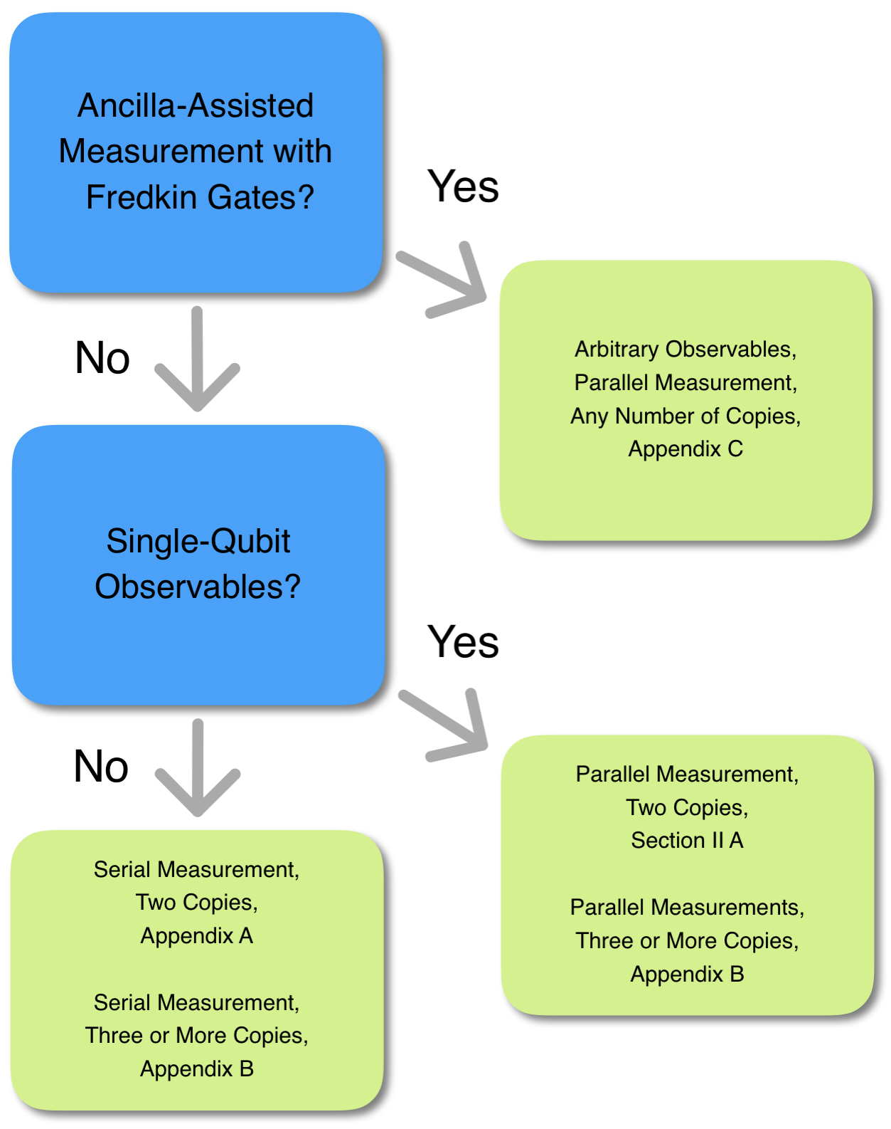
The quantities in the numerator and denominator of Eq. 2 can be evaluated in a number of different ways. For simplicity, we focus our presentation one such approach Section II.1. In that section, we roughly follow the work of Ref. 35, except that we use the language of qubits rather than bosonic systems. We discuss a variety of alternative protocols in Appendix A, Appendix B, and Appendix C. Figure 2 summarizes the differences between these variants. The practical utility of these techniques as error-mitigation tools will be partly determined by the number of samples necessary to evaluate the corrected expectation values to within some target precision . We address this issue in Section II.2 and also show that their exists generalizations of our approach that can further reduce the number of circuit repetitions for a desired precision.
II.1 Measurement by Diagonalization
In this section, we present a straightforward strategy applicable when the operator is the Pauli operator acting on a single qubit and . Other single-qubit observables can be accessed by applying the appropriate single-qubit rotations before the virtual distillation procedure. This realization of our error mitigation technique requires only a single additional layer of two-qubit gates followed by measurement in the computational basis. We present a schematic of this approach in Figure 3.

Rather than using the relation in Eq. 3 directly, we instead define a symmetrized version of our observable,
| (6) |
For the specific case we consider here, that means we take
| (7) |
It is straightforward to use Eq. 3 to show that
| (8) |
Using the symmetrized observable is advantageous because
| (9) |
or, in our case, .
Both and factorize into tensor products of operators that act separately on each pair of qubits, where the th pair consists of the th qubit from each system. Therefore, we may simultaneously diagonalize and using an operator that factorizes with the same structure. We denote the two-qubit unitary that performs this diagonalization on the th pair . We give a matrix representation for this gate below, noting that there is some freedom in the choice of phases for the matrix elements,
| (10) |
We then define
| (11) |
As desired, this unitary diagonalized the individual factors that make up the observables,
| (12) | ||||
| (13) |
This diagonalization is particularly easy to implement when each qubit from the first copy of is adjacent to the corresponding qubit from the second copy. The procedure for measuring the observables required to estimate the numerator and denominator of Eq. 8 then reduces to applying a single layer of two-qubit gates in parallel and measuring in the computational basis. In fact, because diagonalizes for all values of , we naturally collect the data required to estimate the error-mitigated expectation values for all of the operators simultaneously. By applying the appropriate single-qubit rotations before performing virtual distillation, we could instead access an arbitrary single-qubit observable on each qubit. We capture this process diagrammatically in Figure 3.
In order to develop some intuition, it is helpful to express using a spectral decomposition of and consider two separate components of the resulting sum,
| (14) | ||||
The calculation of measurement probabilities and expectation values is a linear operation on the density matrix; we can therefore consider these two components separately. The component of the state with is in the eigenspace of and leads to measurements of which yield the eigenvalue with probability . In the case where , is an even superposition of symmetric and anti-symmetric states,
| (15) |
For this component of the state, measurements of yield and with equal probability and . Combining these two cases, we have the expected equality, . Measurements of follow a similar pattern.
We find it interesting to contrast this behavior with the stabilizer theory of quantum error correction. In the stabilizer formalism, errors are detected by projecting through measurement into the eigenspace of one or more symmetries. In our approach, we instead rely on errors being equally supported on the eigenspaces of the symmetry we measure.
II.2 Sample Efficiency
The number of circuit repetitions required to determine the error-mitigated expectation values within a precision depends on the variance of our estimator. In this section, we present expressions for this variance. We focus on the case and the methods discussed in Section II.1. The calculations are also applicable to the variant protocol we present in Appendix C. We also show how their exists an extension to our protocol that makes more efficient use of multiple copies when the noise level is sufficiently high.
We’d like to determine the variance of our estimator for the error-mitigated expectation value
| (16) |
We leave the derivation to Appendix D and simply give an (approximate) expression for the variance,
| (17) | ||||
where refers to the number of measurement repetitions. It’s useful to consider what happens in the limit where is a pure state. In that case, the second and third lines are zero and the variance reduces to
| (18) |
exactly what one would expect when averaging independent measurements of . As the purity of decreases, the variance, and the number of circuit repetitions, increases.
The rest of this section focuses on laying the groundwork to improve the sample efficiency of these techniques. This is an important goal because the number of samples required can grow large given sufficiently noisy circuits. At high enough error rates, we are highly likely to find ourselves in a situation where
| (19) |
We now make the assumption that the level of error mitigation offered by measuring is sufficient but we have copies of available. For simplicity, we focus on the case where and is a Pauli operator acting on one or more qubits. We present a generalization of our approach involving a collective measurement of all copies of that performs better than a naive parallelization.
The naive approach we hope to beat consists of taking pairs and running the protocol described above in parallel, averaging the results. For simplicity, we focus on the variance of our estimator for the quantity that appears in the numerator of Eq. 8 rather than the ratio itself. In Appendix D we show that the variance of our estimator for is . Therefore, the variance obtained when using copies in parallel is exactly
| (20) |
We prove below that it is possible in some situations to obtain a more sample-efficient estimator for the corrected expectation value by performing a joint measurement on all copies. We do so by providing an operator with the desired expectation value and calculating its variance.
First, we define the operator
| (21) |
where we use to denote the swap operator specifically between subsystems and . It is simple to show that
| (22) |
We compute the variance of with respect to the state in Appendix E, finding that
| (23) |
When is small, the second term in Eq. 23 is suppressed and there is a regime where the variance of this operator shrinks quadratically with . The naive approach, where we perform independent calculations on separate pairs results in an estimator whose variance is suppressed only linearly in . We do not suggest a particular strategy, let alone one that is NISQ-friendly, for implementing the measurement of . We hope that future work can address this issue. Furthermore, while we have established that generalizations of the simplest virtual distillation procedure can outperform a naive parallel strategy, we have not established a comprehensive theory on the limitations of virtual distillation. It would be useful to quantify the minimum number of samples required to resolve given access to a large number of copies of under various assumptions about the spectrum of the density matrix.
III Performance Under Different Noise Models
In the numerical studies, we will present evidence that the performance of virtual distillation can be essentially predicted by the combination of two contributions. Here we find it instructive to consider them separately using simple analytical models. To understand the potential benefit of our approach using the minimal setup, we consider the fidelity of
| (24) |
with the ideal state generated by noiseless evolution (neglecting error introduced by the measurement procedure). We first consider the performance under noise that maps the ideal state to states orthogonal to it, leaving the dominant eigenvector of the density matrix as the ideal state. We then turn towards the effect of errors that lead to states non-orthogonal to the ideal state, causing a drift in the dominant eigenvector of the density matrix. The essential behavior of virtual distillation is to remove errors of the first kind rapidly, while converging to a floor determined by the drift in the dominant eigenvector that enables a large constant factor improvement over the erred state.
III.1 Orthogonal Errors
We first consider idealized errors that leave the dominant eigenvector as the ideal state. We consider a phenomenological error model motivated by the assumption that we can think of errors as discrete events that occur locally in space and time with some probability. For simplicity, we model every gate as a stochastic quantum map where with probability an error occurs, and we assume that every new error sends the quantum evolution to a new orthogonal state. The resulting density matrix for a circuit with gates is
| (25) |
The operator for is similar with all the coefficients squared, as all the states are assumed to be orthogonal. Therefore,
| (26) |
The fidelity with the ideal state is
| (27) | ||||
| (28) |
Therefore we expect a quadratic suppression of errors in the most favorable case.
The result is similar in the case of copies:
| (29) | ||||
| (30) |
The other factor affecting the performance of virtual distillation besides the fidelity is the sample complexity. We analyze the general case in more detail in Appendix D, but it is instructive to briefly consider the performance under this simplified model of errors. For simplicity, we assume that we aim to measure the error-mitigated expectation value of a Pauli operator at the level using independent experiments to estimate the numerator and denominator of Eq. 16 (for a total of experiments). Then the variance of our estimators for the numerator and denominator are upper bounded by , and we have
| (31) |
Because of our assumption that is a Pauli operator, and therefore , we have , implying . Therefore,
| (32) |
When is small, we can neglect the term in the denominator. Therefore, taking
| (33) |
is sufficient to estimate to within a fixed additive error.
III.2 Non-Orthogonal Error Floor
The analysis of the previous section made the simplifying assumption that the dominant eigenvector of the density matrix, , corresponds exactly to the ideal state generated by noiseless evolution. In practice, errors will lead to population in states that may not be orthogonal to the target state, leading to a drift in the dominant eigenvector of the density matrix. We will see in our numerical studies that this drift limits the maximum potential upside of virtual distillation. In this second, we develop an understanding of this drift by using perturbation theory to consider the first-order change in the dominant eigenvector of the density matrix.
Let us consider a state in the middle of a noisy preparation circuit, allowing for to already be somewhat distorted by noise. Writing in its eigenbasis, we have
| (34) |
where we order the eigenvalues in descending order. Note that we use the symbol for the th eigenvector of the density matrix rather than throughout this section, reserving the symbol for the coefficients associated with a Kraus operator decomposition of our noise channel. We wish to consider the impact of a subsequent noise channel defined in terms of a set of Kraus operators,
| (35) |
Note that we have demanded a representation of the channel where is the identity matrix in order to simplify our analysis. Now let denote the change in the density matrix induced by this channel (),
| (36) |
where we define the scale by taking to be .
Now we make the assumption that we are in the low-error regime. Specifically, we assume that and that . Under this assumption, we satisfy the necessary conditions for applying matrix perturbation theory to the dominant eigenvector Kato 2013. We can therefore proceed by expressing the dominant eigenvector of as a convergent power series in . This yields
| (37) |
where denotes the dominant eigenvector of , denotes the dominant eigenvector of the unperturbed , and denotes the correction at th order. Likewise, we can also express the eigenvalue corresponding to the dominant eigenvector as a power series in ,
| (38) |
We can then proceed in the usual way, expanding the eigenvalue equation,
| (39) |
and equating terms order by order. This leads to a familiar expression for the first order correction to the dominant eigenvector in terms of the zeroth order eigenvalues and eigenvectors,
| (40) |
At this point, it’s useful to carefully consider the normalization of . Let denote the normalized form of ,
| (41) |
where we have made use of the fact that the first and second order corrections are both orthogonal to the unperturbed eigenvector.
We can now compute the trace distance between and the dominant eigenvector of the unperturbed state,
| (42) |
Now let us expand in terms of the Kraus operators of our noise model.
| (43) |
where we omit the superscripts of the eigenvalues and eigenvectors on the right-hand side for readability.
We can see that, in the general case, we expect a non-zero contribution to the trace distance at first order in . Because in the low-noise regime, this will effectively set a floor for how well our method can correct errors. Therefore, without further constraints on the state, the noise model, or the observables being measured, our method will not achieve a quadratic suppression in errors in the low noise limit but rather a constant factor improvement whose magnitude depends on the typical size of a quantity we denote by the symbol ,
| (44) |
Interestingly, when we examine the data from our numerical simulations, we do obtain an improvement consistent with a quadratic suppression of errors at intermediate error rates. Additionally, has no lower bound; it can in some cases be zero, in which case we expect to recover the quadratic suppression of error predicted from Section III.1. As the trace distance is an upper bound for the error in any observable, particular observables of particular states may recover this performance even when .
In order to shed some light on the error floor set by the drift in the dominant eigenvector of the density matrix, it can be helpful to ask when we might expect to be near zero. It is clear that this quantity must be zero if one of two conditions hold:
| (45) | ||||
| (46) |
One way that this can occur is if the state and the circuit have a natural set of symmetries. The first condition holds if the error is drawn from such a symmetry group, while the second is satisfied if it violates it strictly. For an example of the second case, consider a bit-flip or amplitude-damping error channel acting on a state with a definite number of excitations. There are other situations where the second equality is approximately satisfied. For example, in circuits exhibiting the limits of quantum chaos, apart from a small light cone at the end of the circuit, any local errors lead to a state nearly indistinguishable from a Haar random state. Therefore, the matrix elements in Eq. 46 are exponentially small in the number of qubits. This sensitivity to local perturbations in random circuits is used in the cross-entropy benchmarking technique Arute et al. 2019, and explains the improved behavior of our technique in numerical tests on random circuits.
IV Numerical Experiments
In this section, we present numerical simulations of virtual distillation applied to three model systems. We first consider two classes of random circuits, chosen because they are simple limits where the behaviour of virtual distillation is easy to analyze. We then turn towards the application of virtual distillation to the simulation of the dynamics of a one dimensional spin chain following a quantum quench. This example allows us to study the behaviour of virtual distillation in the context of quantum simulation, an application which is a promising candidate for the eventual demonstration of practical quantum advantage in the NISQ era. We choose to focus on time evolution rather than the ground state problem mainly because ground states have additional structure which enables specialized error mitigation techniques and we are interested in how virtual distillation behaves in the absence of this structure.
We find it illuminating to characterize the effectiveness of our approach as a function of the expected number of errors in a particular circuit. This tends to allow more universal prediction of performance when trading between error rate per gate and number of gates. We consider a noise model that focuses on stochastic errors in two-qubit gates. Specifically, after each two-qubit gate, we apply a single-qubit depolarizing channel to both qubits acted on by the gate. The expected number of errors () can be expressed simply as a function of the number of two-qubit gates in the circuit () and the single-qubit depolarizing probability (, defined in the usual way in Eq. 95),
| (47) |
To quantify the error, we focus mainly on the trace distance between the ideal state that would be obtained with noise-free evolution and the effective state accessed by virtual distillation The trace distance leads to a natural bound in the error for the expectation value of an arbitrary observable,
| (48) |
where is an observable with operator norm , and denotes the trace distance.
IV.1 Scrambling Circuits
Both classes of random circuits that we simulate are related to the scrambling circuits used to demonstrate beyond classical computation in Ref. 44. The first class is essentially a one-dimensional version of the circuit family considered in that work. The second class of circuits is exactly the same as the first class, except that we remove the two-qubit gates. We provide some additional details in Appendix F. For these non-entangling random circuits, we still perform the noisy simulations of these circuits by applying single-qubit depolarizing channels in the same locations where the two-qubit gates would have been.
Because the behaviour of the non-entangling random circuits is particularly simple to understand, we consider this class of circuits first. In the absence of entangling gates, we can commute the applications of the single-qubit depolarizing channel to the end of the circuit. We can then combine them together into a single application per qubit with a larger effective error rate. We carry this procedure out analytically in Appendix F, showing that the dominant eigenvector of the density matrix corresponds exactly the ideal state. This leads us to expect behaviour similar to that of the phenomenological noise model we considered in Section III.1.

In Figure 4, we plot the trace distances between the ideal states generated by noiseless evolution and the states obtained by noisy evolution of these non-entangling random circuits (blue curve). We consider a variety of different circuit depths and error rates for both six-qubit systems (thin curves) and ten qubit systems (thick curves). For each of these simulations, we also calculate the trace distance between the ideal state and the states we are effectively accessing by using virtual distillation with (orange dotted curve, ) or (green dotted curve, ) copies. For each particular setting of circuit depth and error rate, we consider a single randomly chosen member from the ensemble of non-entangling scrambling circuits described above.
We see that the data from this variety of simulations collapses together when we plot the error (in terms of trace distance) as a function of the expected number of gate errors. When the expected number of errors is not too large, the curves for , , and are nearly linear with slopes , , and respectively. Although the noise model in this case does not exactly match the phenomenological model of Section III.1, the results are broadly consistent. For these non-entangling random circuits, we observe a level of error suppression that is exponential in .

In Figure 5 and Figure 6, we present plots that explore the behaviour of entangling random circuits on a one-dimensional line of qubits. When we considered the non-entangling random circuits, we found that error (quantified by the trace distance to the ideal state) depended mostly on the system size and the expected number of gate errors. This was true regardless of whether or the expected number of errors was varied by changing the circuit depth or by changing the error rate per-gate. Here we observe slightly different behaviour between these two cases, and therefore consider them separately. These two figures also differ from Figure 4 in that they include a red dashed curve corresponding to trace distance between the dominant eigenvector of the density matrix () and the ideal state, a quantity which is non-zero for the richer family of circuits we now consider.

Figure 5 presents two plots that show the effects of varying the circuit depth at two different fixed error rates. We see that the error in the dominant eigenvector effectively sets a floor for the minimal error achievable by virtual distillation for any value of . This floor grows slowly with increasing circuit depth. Furthermore, both the absolute magnitude and the rate of growth appear to be suppressed with system size. In Section III.2 we showed that the leading order contributions to the trace distance between the dominant eigenvector and the ideal state can be understood in terms of the matrix elements of the Kraus operators (see Eq. 44). As the circuit depth of the random circuit increases, we expect a 1D random circuit to approach a Haar random circuit at a depth proportional to the number of qubits . Once this approximation is sufficient, all but a small fraction of errors in the lightcone of the observable at the end of the circuit will lead to matrix elements that contribute to the drift in the dominant eigenvector that are exponentially small in the number of qubits. This observation may explain the scaling we see in Figure 5.
In Figure 6 we plot the error in terms of trace distance as we vary the expected number of gate errors by varying the per-gate error rate for a fixed circuit. At low error rates, we see that the errors in the dominant eigenvectors (red dashed curves) scale linearly with the error rate but are orders of magnitude smaller than the errors in the unmitigated state. This matches the behaviour we would expect from the analysis of Section III.2. As in Figure 5, the error in the dominant eigenvector sets a floor for the performance of our method at finite and that this floor is suppressed as the system size increases.
IV.2 Heisenberg Quench
The properties of random circuits can be somewhat unique in their ability to scramble errors. It is thus important to consider how the approach works for other circuits of interest, like the quantum simulation of physical systems. In this section, we explore the performance of our approach applied to the simulation of time evolution following a quantum quench in a spin model. We initialize the system in an antiferromagnetic state, e.g., , and simulate the time evolution under the Hamiltonian
| (49) | ||||
Here we have chosen the parameters, , , , in order to match a previously studied family of non-integrable models Dmitriev and Krivnov 2004, although we take open boundary conditions rather than periodic ones. We approximate the time evolution under this Hamiltonian by Trotterization with a timestep of . Specifically, we use alternating layers of single-qubit gates, two-qubit gates between odd-even pairs of qubits, and two-qubit gates between even-odd pairs of qubits. As above, we simulate the resulting circuits with single-qubit depolarizing noise applied after every two-qubit gate.

In Figure 7, we plot the bounds on the error of an arbitrary observable (normalized so that ) derived from the trace distance to the noiseless state. We vary the expected number of errors by varying the circuit depth of a six qubit system with a fixed single-qubit depolarizing probability of . Alongside these bounds (plotted using solid and dashed curves) we also plot the actual average error in the single-site magnetization (averaged over the sites) at various points throughout the circuit. For the two-copy () version of our proposal, we plot the error calculated directly from the state using yellow crosses and the error we would obtain by applying the destructive measurement described in Section II.1 using large purple diamonds. For this second calculation, we simulate the application of the six two-qubit gates (Eq. 10) required to diagonalize the observables using the same noise model as the rest of the circuit. From the nearly perfect overlap of the yellow crosses with the purple diamonds, we can see that circuit noise during the diagonalization step has barely any effect on the reconstructed expectation values. It is also apparent that, although the average error in the magnetization does not saturate the bounds implied by the trace distance, our approach suppresses the errors in the actual expectation values to a similar degree that it suppresses the trace distance.

Figure 8 offers a different look at the same system. As with Figure 6, in this figure we fix the number of two-qubit gates to be and we vary the expected number of gate errors by sweeping over a range of per-gate error rates. Here we clearly see the impact of the floor set by the drift in the dominant eigenvector (red dotted curve). At low gate error rates, the error (in terms of trace distance to the ideal state) for the virtually distilled states () is suppressed by a constant factor relative to the error in the unmitigated state (). The constant factor improvement is substantial and appears to increase with system size. Both the size of the improvement and its sensitivity to the system size are smaller than we observed for the one-dimensional scrambling circuits of Figure 6.

In Figure 9, we consider the cost of performing the two-copy () version of virtual distillation for the same systems considered in Figure 8. We do this using the expression for the variance presented in Eq. 17 and derived in Appendix D. Using this expression, we calculate the average variance of our error-mitigated estimators for the single-site magnetization, . We consider the ratio of this average variance (for the error-mitigated expectation values) with the average variance of the same measurements without error mitigation. Because the number of measurements required for some fixed precision scales linearly with the variance, this ratio is also the ratio between the number of measurements required to use virtual distillation and the number of measurements required to measure the unmitigated expectation values (assuming the same target precision). This quantity therefore encapsulates the overhead incurred by our scheme.
When the expected number of errors is small, we see that virtual distillation barely increases the number of measurements required. It is only as the number of errors grows larger than one that the measurement cost rises dramatically. We note that Eq. 17 implicitly assumes that we perform a number of measurements such that
| (50) |
This assumption will break down when the target precision is low and the expected number of errors in Figure 9 is large, but the qualitative conclusion remains the same.
V Mitigating Algorithmic Errors
To date, most error mitigation methods have focused on the reduction of errors caused by imperfections in a device implementation, such as decoherence or control errors. Here explore the idea that some of these techniques can be applied to algorithmic errors incurred during otherwise noise-free implementations of randomized algorithms. Previous works have used extrapolation Endo et al. 2019 or randomized symmetry application Tran et al. 2020 to mitigate coherent errors in evolution; we extend this concept to incoherent errors.
Recent developments in Hamiltonian simulation have led to the development of randomized evolution methods such as qDRIFT Campbell 2019, randomized Trotter Childs et al. 2019, and combinations thereof Ouyang et al. 2020, which have benefits in some situations over their deterministic counterparts. As these methods are randomized, they output mixed states rather than pure states, even in the absence of noise. Moreover, they depend on an approximation parameter with a natural limit in which they converge to the pure state generated by exact evolution. In this section, we show numerically that virtual distillation applied to qDRIFT can suppress this deviation from the exact evolution. For the particular model system we consider, we find that virtual distillation can reduce the coherent space-time volume required to reach a particular accuracy threshold by a factor of or more compared with the standard qDRIFT.
V.1 qDRIFT
We briefly introduce some background on the qDRIFT method. qDRIFT simulates time evolution under a Hamiltonian , by constructing product formulae using a randomized selection rule. Terms are chosen from at random, with a selection probability proportional to their interaction strength in the Hamiltonian. One then evolves the system forwards in time under this Hamiltonian term, for a fixed timestep and repeats this process a number of times, generating a product formula that provides an approximation to the time evolution operator. When averaged over the classical randomness (in the choice of interaction terms), qDRIFT generates a quantum channel that closely approximates the exact evolution more closely than the individual product formulae. Importantly, unlike most deterministic Trotter methods, the scaling of this approach does not depend explicitly on the number of terms in the Hamiltonian, but rather than -norm of the coefficients.
More precisely, we consider a Hamiltonian that we may decompose as , where all are made real and positive by absorbing signs into , and the spectral norm of is bounded by . Defining , the diamond norm distance between the qDRIFT channel and the true time evolution is bounded by
| (51) |
where is the number of qDRIFT selection steps performed to generate each instance of the qDRIFT channel, and hence controls the amount of coherent evolution required. As increases, the resulting quantum channel converges to the unitary corresponding to the exact evolution. It will be our aim to understand how our virtual distillation technique can reduce the coherent space-time volume required, by reducing this factor required to achieve the same error in practice.

V.2 Virtual distillation applied to qDRIFT
Here we study the application of virtual distillation to qDRIFT numerically. Specifically, we investigate how virtual distillation can impact the number of coherent steps, , required to reach a target accuracy. For this, we choose a Heisenberg Hamiltonian with up to 6 qubits per copy. The Hamiltonian is given by
| (52) |
where are randomly chosen magnetic field strengths, and periodic boundary conditions are applied such that site is site . For our studies here, we choose a time evolution length of and let . We numerically investigate the number of coherent qDRIFT steps required to achieve a trace distance of to the ideal state for evolutions under such a Heisenberg model. The results of this analysis are shown in Fig. 10. We see for this system that virtual distillation consistently reduces the required number of coherent steps to achieve the desired trace distance by a factor of more than x. If we account for the space overhead of using two copies, this still amounts to a space-time advantage of x. These results suggest that the use of error mitigation techniques may be further developed to yield practical algorithmic improvements for real systems, especially in the NISQ regime.
VI Conclusion
In this work, we showed how techniques for using multiple copies of a state to access polynomials of the density matrix can be used to mitigate incoherent errors. We studied the effectiveness of this approach for two analytically tractable noise models and characterized its limit in terms of the dominant eigenvector of the noisy density matrix. We numerically demonstrated reductions in the error (quantified by the trace distance to the noise-free state) of up to three orders of magnitude for a collection of small model systems. Furthermore, we showed that this error suppression is enhanced as the system size or the speed of information scrambling grows. We also considered the application of our error mitigation approach to the incoherent algorithmic error that arises when approximating time-evolution using the qDRIFT algorithm, finding a substantial constant factor improvement.
Our proposed strategy for error mitigation, which we refer to as virtual distillation, is simple to use and analyze. It provides a natural way to take advantage of the surplus of qubits that we expect to have available as the NISQ era continues to suppress the effects of incoherent errors. We expect that our technique will prove complementary to other error mitigation and calibration techniques, especially those capable of addressing coherent errors. The effective state accessed by virtual distillation approaches the dominant eigenvector of the density matrix exponentially quickly as the number of copies, , increases. Therefore, the utility of our technique depends mainly on the error in the dominant eigenvector and the number of samples required. In particular, we have devoted a signficant amount of attention to the question of sample complexity. This is due to the fact that proposed NISQ applications, especially in quantum simulation, already face a daunting cost in this regard Huggins et al. 2019. Our analytical work and numerical simulations indicate that our strategy is most effective and affordable when the number of errors expected in the circuit is . The reach of our approach will therefore naturally grow throughout the NISQ era as hardware platforms continue to improve.
There are several other important considerations relevant to the performance of this technique in the NISQ era besides the drift in the dominant eigenvector and the sample complexity. First of all, virtual distillation requires collective measurements that couple the qubits of one copy with the corresponding qubits of additional copies. For hardware platforms based on a 2D grid of qubits, these measurements are easiest to perform when the connectivity of the original circuit is linear and would require a substantial number of additional gates in the general case. Fortunately, a linearly connected array of qubits is known to be sufficient to achieve the optimal gate complexity in some cases, including certain approaches for the simulation of quantum chemistry Kivlichan et al. 2018; O’Gorman et al. 2019. A second important consideration is that we’re often interested in measuring observables with support on more than one qubit. We discuss some options for performing such measurements in Appendix A, Appendix B, and Appendix C, but these options come with their own overheads in gate complexity or the number of measurements repetitions. Thirdly, and perhaps most importantly, the assumption that we’re able to measure expectation values with respect to is violated when the individual copies are not in the same state or when errors occur during execution of the measurements. We discuss some aspects of the breakdown of this assumption in Appendix H. In general, we do not expect virtual distillation to be able to correct errors during the measurement process but we note that we saw a reasonable level of robustness to such errors in our numerical simulations (see Figure 7).
Even as we begin to leave the NISQ era behind and approach devices that start to incorporate quantum error correction, in the early days the desire to use as many logical qubits as possible means we may perform some computations that still have an appreciable number of logical errors. Given that our technique can provide a substantial improvement in error at negligible overhead compared to traditional quantum error correction techniques, there may be some advantageous interplay between the two, where small distance codes are used in conjunction with this technique before more qubits are available. We explore this opportunity in more detail in Appendix G.
Our technique builds upon a long tradition of work that uses the symmetric group for stabilizing quantum computations and mitigating errors. We believe that this research direction continues to hold promise, and we identify a few directions that we find particularly intriguing. Virtual distillation is based on a simple collective measurement of copies of . In Section II.2, we show that there exists more sophisticated collective measurements whose sample complexity improves quadratically upon our approach in some regimes. It would be interesting to investigate this further, both from a fundamental perspective, and with an eye towards practical implementation. Besides this potential improvement, another clear question arises from our work. The drift in the dominant eigenvector of the density matrix is a coherent error. As with the coherent errors that occur directly in the execution of circuits on a NISQ device, we are hopeful that variational optimization or other, complementary, error mitigation techniques may prove useful in addressing this additional source of coherent error. Studying this in the context of the real noise experienced in hardware will be especially important and illuminating.
In the process of preparing this work, a related paper, Ref. 53 appeared in the literature. Our work highlights different conclusions than theirs in error scaling due to our explicit consideration of errors that induce a drift in the dominant eigenvector of the density matrix.
Acknowledgements
The authors are extremely grateful to Dave Bacon for key discussions around the symmetric subspace and diagrammatic derivations, Gian-Luca Anselmetti for suggestions around performing virtual distillation with two distinct states, and Nathan Wiebe for helpful advice at various stages. WJH and KBW acknowledge support from the NSF QLCI program through grant number OMA-2016245.
References
- Aharonov and Ben-Or (1997) D Aharonov and M Ben-Or, “Fault-tolerant quantum computation with constant error,” in Proceedings of the twenty-ninth annual ACM symposium on Theory of computing, STOC ’97 (Association for Computing Machinery, New York, NY, USA, 1997) pp. 176–188.
- Fowler et al. (2012) Austin G Fowler, Matteo Mariantoni, John M Martinis, and Andrew N Cleland, “Surface codes: Towards practical large-scale quantum computation,” Phys. Rev. A 86, 032324 (2012).
- Preskill (2018) John Preskill, “Quantum computing in the NISQ era and beyond,” Quantum 2, 79 (2018).
- Temme et al. (2017) Kristan Temme, Sergey Bravyi, and Jay M Gambetta, “Error mitigation for Short-Depth quantum circuits,” Phys. Rev. Lett. 119, 180509 (2017).
- Endo et al. (2018) Suguru Endo, Simon C Benjamin, and Ying Li, “Practical quantum error mitigation for Near-Future applications,” Phys. Rev. X 8, 031027 (2018).
- Kandala et al. (2019) Abhinav Kandala, Kristan Temme, Antonio D Córcoles, Antonio Mezzacapo, Jerry M Chow, and Jay M Gambetta, “Error mitigation extends the computational reach of a noisy quantum processor,” Nature 567, 491–495 (2019).
- Strikis et al. (2020) Armands Strikis, Dayue Qin, Yanzhu Chen, Simon C Benjamin, and Ying Li, “Learning-based quantum error mitigation,” arXiv:2005.07601 (2020).
- Czarnik et al. (2020) Piotr Czarnik, Andrew Arrasmith, Patrick J Coles, and Lukasz Cincio, “Error mitigation with clifford quantum-circuit data,” arXiv:2005.10189 (2020).
- Arute et al. (2020) Frank Arute, Kunal Arya, Ryan Babbush, Dave Bacon, Joseph C Bardin, Rami Barends, Andreas Bengtsson, Sergio Boixo, Michael Broughton, Bob B Buckley, David A Buell, Brian Burkett, Nicholas Bushnell, Yu Chen, Zijun Chen, Yu-An Chen, Ben Chiaro, Roberto Collins, Stephen J Cotton, William Courtney, Sean Demura, Alan Derk, Andrew Dunsworth, Daniel Eppens, Thomas Eckl, Catherine Erickson, Edward Farhi, Austin Fowler, Brooks Foxen, Craig Gidney, Marissa Giustina, Rob Graff, Jonathan A Gross, Steve Habegger, Matthew P Harrigan, Alan Ho, Sabrina Hong, Trent Huang, William Huggins, Lev B Ioffe, Sergei V Isakov, Evan Jeffrey, Zhang Jiang, Cody Jones, Dvir Kafri, Kostyantyn Kechedzhi, Julian Kelly, Seon Kim, Paul V Klimov, Alexander N Korotkov, Fedor Kostritsa, David Landhuis, Pavel Laptev, Mike Lindmark, Erik Lucero, Michael Marthaler, Orion Martin, John M Martinis, Anika Marusczyk, Sam McArdle, Jarrod R McClean, Trevor McCourt, Matt McEwen, Anthony Megrant, Carlos Mejuto-Zaera, Xiao Mi, Masoud Mohseni, Wojciech Mruczkiewicz, Josh Mutus, Ofer Naaman, Matthew Neeley, Charles Neill, Hartmut Neven, Michael Newman, Murphy Yuezhen Niu, Thomas E O’Brien, Eric Ostby, Bálint Pató, Andre Petukhov, Harald Putterman, Chris Quintana, Jan-Michael Reiner, Pedram Roushan, Nicholas C Rubin, Daniel Sank, Kevin J Satzinger, Vadim Smelyanskiy, Doug Strain, Kevin J Sung, Peter Schmitteckert, Marco Szalay, Norm M Tubman, Amit Vainsencher, Theodore White, Nicolas Vogt, Z Jamie Yao, Ping Yeh, Adam Zalcman, and Sebastian Zanker, “Observation of separated dynamics of charge and spin in the Fermi-Hubbard model,” arXiv:2010.07965 (2020).
- O’Brien et al. (2020) Thomas E O’Brien, Stefano Polla, Nicholas C Rubin, William J Huggins, Sam McArdle, Sergio Boixo, Jarrod R McClean, and Ryan Babbush, “Error mitigation via verified phase estimation,” arXiv:2010.02538 (2020).
- McClean et al. (2017) Jarrod R McClean, Mollie E Kimchi-Schwartz, Jonathan Carter, and Wibe A de Jong, “Hybrid quantum-classical hierarchy for mitigation of decoherence and determination of excited states,” Phys. Rev. A 95, 042308 (2017).
- Colless et al. (2018) J I Colless, V V Ramasesh, D Dahlen, M S Blok, M E Kimchi-Schwartz, J R McClean, J Carter, W A de Jong, and I Siddiqi, “Computation of molecular spectra on a quantum processor with an Error-Resilient algorithm,” Phys. Rev. X 8, 011021 (2018).
- McClean et al. (2020) Jarrod R McClean, Zhang Jiang, Nicholas C Rubin, Ryan Babbush, and Hartmut Neven, “Decoding quantum errors with subspace expansions,” Nat. Commun. 11, 636 (2020).
- Bonet-Monroig et al. (2018) X Bonet-Monroig, R Sagastizabal, M Singh, and T E O’Brien, “Low-cost error mitigation by symmetry verification,” Phys. Rev. A 98, 062339 (2018).
- McArdle et al. (2019) Sam McArdle, Xiao Yuan, and Simon Benjamin, “Error-Mitigated digital quantum simulation,” Phys. Rev. Lett. 122, 180501 (2019).
- Sagastizabal et al. (2019) R Sagastizabal, X Bonet-Monroig, M Singh, M A Rol, C C Bultink, X Fu, C H Price, V P Ostroukh, N Muthusubramanian, A Bruno, M Beekman, N Haider, T E O’Brien, and L DiCarlo, “Experimental error mitigation via symmetry verification in a variational quantum eigensolver,” Phys. Rev. A 100, 010302 (2019).
- Huggins et al. (2019) William J Huggins, Jarrod McClean, Nicholas Rubin, Zhang Jiang, Nathan Wiebe, K Birgitta Whaley, and Ryan Babbush, “Efficient and noise resilient measurements for quantum chemistry on Near-Term quantum computers,” arXiv:1907.13117 (2019).
- Google AI Quantum and Collaborators (2020) Google AI Quantum and Collaborators, “Hartree-Fock on a superconducting qubit quantum computer,” Science 369, 1084–1089 (2020).
- Chen et al. (2019) Yanzhu Chen, Maziar Farahzad, Shinjae Yoo, and Tzu-Chieh Wei, “Detector tomography on IBM quantum computers and mitigation of an imperfect measurement,” Phys. Rev. A 100, 052315 (2019).
- Maciejewski et al. (2020) Filip B Maciejewski, Zoltán Zimborás, and Michał Oszmaniec, “Mitigation of readout noise in near-term quantum devices by classical post-processing based on detector tomography,” Quantum 4, 257 (2020).
- Bravyi et al. (2020) Sergey Bravyi, Sarah Sheldon, Abhinav Kandala, David C Mckay, and Jay M Gambetta, “Mitigating measurement errors in multi-qubit experiments,” (2020), arXiv:2006.14044 [quant-ph] .
- Berthiaume et al. (1994) A Berthiaume, D Deutsch, and R Jozsa, “The stabilisation of quantum computations,” in Proceedings Workshop on Physics and Computation. PhysComp ’94 (ieeexplore.ieee.org, 1994) pp. 60–62.
- Barenco et al. (1997) Adriano Barenco, André Berthiaume, David Deutsch, Artur Ekert, Richard Jozsa, and Chiara Macchiavello, “Stabilization of quantum computations by symmetrization,” SIAM J. Comput. 26, 1541–1557 (1997).
- Peres (1999) Asher Peres, “Error symmetrization in quantum computers,” Int. J. Theor. Phys. 38, 799–805 (1999).
- Horodecki and Ekert (2002) Paweł Horodecki and Artur Ekert, “Method for direct detection of quantum entanglement,” Phys. Rev. Lett. 89, 127902 (2002).
- Ekert et al. (2002) Artur K Ekert, Carolina Moura Alves, Daniel K L Oi, Michał Horodecki, Paweł Horodecki, and L C Kwek, “Direct estimations of linear and nonlinear functionals of a quantum state,” Phys. Rev. Lett. 88, 217901 (2002).
- Brun (2004) Todd A Brun, “Measuring polynomial functions of states,” arXiv:quant-ph/0401067 (2004).
- Hastings et al. (2010) Matthew B Hastings, Iván González, Ann B Kallin, and Roger G Melko, “Measuring renyi entanglement entropy in quantum monte carlo simulations,” Phys. Rev. Lett. 104, 157201 (2010).
- Islam et al. (2015) Rajibul Islam, Ruichao Ma, Philipp M Preiss, M Eric Tai, Alexander Lukin, Matthew Rispoli, and Markus Greiner, “Measuring entanglement entropy in a quantum many-body system,” Nature 528, 77–83 (2015).
- Garcia-Escartin and Chamorro-Posada (2013) Juan Carlos Garcia-Escartin and Pedro Chamorro-Posada, “SWAP test and Hong-Ou-Mandel effect are equivalent,” Phys. Rev. A 87, 052330 (2013).
- Johri et al. (2017) Sonika Johri, Damian S Steiger, and Matthias Troyer, “Entanglement spectroscopy on a quantum computer,” Phys. Rev. B Condens. Matter 96, 195136 (2017).
- Subaşı et al. (2019) Yiğit Subaşı, Lukasz Cincio, and Patrick J Coles, “Entanglement spectroscopy with a depth-two quantum circuit,” J. Phys. A: Math. Theor. 52, 044001 (2019).
- Banchi et al. (2016) Leonardo Banchi, Abolfazl Bayat, and Sougato Bose, “Entanglement entropy scaling in solid-state spin arrays via capacitance measurements,” Phys. Rev. B Condens. Matter 94, 241117 (2016).
- Bacon et al. (2006) Dave Bacon, Isaac L Chuang, and Aram W Harrow, “Efficient quantum circuits for schur and Clebsch-Gordan transforms,” Phys. Rev. Lett. 97, 170502 (2006).
- Cotler et al. (2019) Jordan Cotler, Soonwon Choi, Alexander Lukin, Hrant Gharibyan, Tarun Grover, M Eric Tai, Matthew Rispoli, Robert Schittko, Philipp M Preiss, Adam M Kaufman, Markus Greiner, Hannes Pichler, and Patrick Hayden, “Quantum virtual cooling,” Phys. Rev. X 9, 031013 (2019).
- Bravyi and Kitaev (2005) Sergey Bravyi and Alexei Kitaev, “Universal quantum computation with ideal clifford gates and noisy ancillas,” Phys. Rev. A 71, 022316 (2005).
- Knill (2005) E Knill, “Quantum computing with realistically noisy devices,” Nature 434, 39–44 (2005).
- Haah and Hastings (2018) Jeongwan Haah and Matthew B Hastings, “Codes and protocols for distilling T , controlled- S , and toffoli gates,” Quantum 2, 71 (2018).
- Cirac et al. (1999) J I Cirac, A K Ekert, and C Macchiavello, “Optimal purification of single qubits,” Phys. Rev. Lett. 82, 4344–4347 (1999).
- Biamonte and Bergholm (2017) Jacob Biamonte and Ville Bergholm, “Tensor networks in a nutshell,” arXiv:1708.00006 (2017).
- Bridgeman and Chubb (2017) Jacob C Bridgeman and Christopher T Chubb, “Hand-waving and interpretive dance: an introductory course on tensor networks,” J. Phys. A: Math. Theor. 50, 223001 (2017).
- Orus (2014) Roman Orus, “A practical introduction to tensor networks: Matrix product states and projected entangled pair states,” Ann. Phys. 349, 117–158 (2014).
- Kato (2013) Tosio Kato, Perturbation theory for linear operators (Springer Science & Business Media, 2013).
- Arute et al. (2019) Frank Arute, Kunal Arya, Ryan Babbush, Dave Bacon, Joseph C Bardin, Rami Barends, Rupak Biswas, Sergio Boixo, Fernando G S L Brandao, David A Buell, Brian Burkett, Yu Chen, Zijun Chen, Ben Chiaro, Roberto Collins, William Courtney, Andrew Dunsworth, Edward Farhi, Brooks Foxen, Austin Fowler, Craig Gidney, Marissa Giustina, Rob Graff, Keith Guerin, Steve Habegger, Matthew P Harrigan, Michael J Hartmann, Alan Ho, Markus Hoffmann, Trent Huang, Travis S Humble, Sergei V Isakov, Evan Jeffrey, Zhang Jiang, Dvir Kafri, Kostyantyn Kechedzhi, Julian Kelly, Paul V Klimov, Sergey Knysh, Alexander Korotkov, Fedor Kostritsa, David Landhuis, Mike Lindmark, Erik Lucero, Dmitry Lyakh, Salvatore Mandrà, Jarrod R McClean, Matthew McEwen, Anthony Megrant, Xiao Mi, Kristel Michielsen, Masoud Mohseni, Josh Mutus, Ofer Naaman, Matthew Neeley, Charles Neill, Murphy Yuezhen Niu, Eric Ostby, Andre Petukhov, John C Platt, Chris Quintana, Eleanor G Rieffel, Pedram Roushan, Nicholas C Rubin, Daniel Sank, Kevin J Satzinger, Vadim Smelyanskiy, Kevin J Sung, Matthew D Trevithick, Amit Vainsencher, Benjamin Villalonga, Theodore White, Z Jamie Yao, Ping Yeh, Adam Zalcman, Hartmut Neven, and John M Martinis, “Quantum supremacy using a programmable superconducting processor,” Nature 574, 505–510 (2019).
- Dmitriev and Krivnov (2004) D V Dmitriev and V Ya Krivnov, “Quasi-one-dimensional anisotropic heisenberg model in a transverse magnetic field,” Journal of Experimental and Theoretical Physics Letters 80, 303–307 (2004).
- Endo et al. (2019) Suguru Endo, Qi Zhao, Ying Li, Simon Benjamin, and Xiao Yuan, “Mitigating algorithmic errors in a hamiltonian simulation,” Phys. Rev. A 99, 012334 (2019).
- Tran et al. (2020) Minh C Tran, Yuan Su, Daniel Carney, and Jacob M Taylor, “Faster digital quantum simulation by symmetry protection,” arXiv:2006.16248 (2020).
- Campbell (2019) Earl Campbell, “Random compiler for fast hamiltonian simulation,” Phys. Rev. Lett. 123, 070503 (2019).
- Childs et al. (2019) Andrew M Childs, Aaron Ostrander, and Yuan Su, “Faster quantum simulation by randomization,” Quantum 3, 182 (2019).
- Ouyang et al. (2020) Yingkai Ouyang, David R White, and Earl T Campbell, “Compilation by stochastic Hamiltonian sparsification,” Quantum 4, 235 (2020).
- Kivlichan et al. (2018) Ian D Kivlichan, Jarrod McClean, Nathan Wiebe, Craig Gidney, Alán Aspuru-Guzik, Garnet Kin-Lic Chan, and Ryan Babbush, “Quantum simulation of electronic structure with linear depth and connectivity,” Phys. Rev. Lett. 120, 110501 (2018).
- O’Gorman et al. (2019) Bryan O’Gorman, William J Huggins, Eleanor G Rieffel, and K Birgitta Whaley, “Generalized swap networks for near-term quantum computing,” (2019), arXiv:1905.05118 [quant-ph] .
- Koczor (2020) Bálint Koczor, “Exponential error suppression for Near-Term quantum devices,” arXiv:2011.05942 (2020).
- Cotler and Wilczek (2020) Jordan Cotler and Frank Wilczek, “Quantum overlapping tomography,” Phys. Rev. Lett. 124, 100401 (2020).
- Bonet-Monroig et al. (2020) Xavier Bonet-Monroig, Ryan Babbush, and Thomas E O’Brien, “Nearly optimal measurement scheduling for partial tomography of quantum states,” Phys. Rev. X 10, 031064 (2020).
- Yu. Kitaev (1995) A Yu. Kitaev, “Quantum measurements and the abelian stabilizer problem,” arXiv:quant-ph/9511026 (1995).
- Kendall and Others (1946) Maurice George Kendall and Others, The Advanced Theory of Statistics (Charles Griffin and Co., Ltd., London, 1946).
- Wang et al. (2010) D S Wang, A G Fowler, A M Stephens, and L C L Hollenberg, “Threshold error rates for the toric and planar codes,” Quantum Inf. Comput. 10, 456–469 (2010).
- Horsman et al. (2012) Clare Horsman, Austin G Fowler, Simon Devitt, and Rodney Van Meter, “Surface code quantum computing by lattice surgery,” New J. Phys. 14, 123011 (2012).
- Litinski (2019) Daniel Litinski, “A Game of Surface Codes: Large-Scale Quantum Computing with Lattice Surgery,” Quantum 3, 128 (2019).
- Preskill (1998) John Preskill, “Lecture notes for physics 229: Quantum information and computation,” (1998).
- Krantz et al. (2019) P Krantz, M Kjaergaard, F Yan, T P Orlando, S Gustavsson, and W D Oliver, “A quantum engineer’s guide to superconducting qubits,” Applied Physics Reviews 6, 021318 (2019).
Appendix A Measuring Multi-Qubit Observables by Diagonalization
In Section II.1, we presented a straightforward strategy for applying the version of virtual distillation to single-qubit observables. Measuring observables with support on more than one qubit is more challenging. Ref. 35 solved this issue by using an approach like the one we describe below in Appendix C. Alternatively, one could apply a circuit to localize an observable of interest to a single qubit before performing virtual distillation. Here we present an alternative solution that doesn’t require the use of ancilla-assisted measurement or circuit depth.
The challenge arises due to the use of Eq. 8, in particular, the choice to use the symmetrized version of an observable, a notion defined in Eq. 6. Using the symmetrized version of a multi-qubit observable means that it is not possible to perform the required diagonalization using a tensor product of separate unitaries across each pair of qubits. As an example, we consider the operator . Our arguments hold equally well for any other operator composed of a tensor product of (more than one) single-qubit Pauli operators. Taking the product of the symmetrized observable and the swap operator yields
| (53) |
This operator does not factorize into a tensor product of operators with support on the individual pairs of qubits, nor can it be diagonalized by an operator that factors this way.
However, instead of using Eq. 8 to determine the corrected expectation value of , we can instead use the non-symmetrized form introduced in Eq. 2. Returning to our example where , we see that we need to estimate the numerator and denominator of
| (54) |
Unlike the symmetrized observable of Eq. 53, the operator factorizes into a tensor product over the pairs of qubits (a pair being one qubit from the first system and the corresponding qubit from the second system). is not Hermitian, but because it is unitary, we can still estimate by applying a circuit to diagonalize it and measuring in the computational basis. As factorizes into a product of two-qubit operators, the circuit that diagonalizes it does as well.
Note that because does not commute with , we will be unable to simultaneously estimate the numerator and denominator of Eq. 54. We will also be unable to simultaneously measure the corrected expectation value corresponding to different choices of and . More generally, we are able to measure any single tensor product of one-qubit operators at a time, regardless of the number of qubits it acts on. The details of the diagonalization will, of course, depend upon the operator to be measured. We do not carefully analyze the number of measurements required by this flavor of virtual distillation, but we note that the inability to parallelize the measurement of commuting multi-qubit observables would make it challenging to profitably combine this approach with sophisticated NISQ measurement strategies, such as the one presented in Ref. 17. In particular, individual multi-qubit operator must be measured separately using this approach, even if they commute. This fact increases the overall number of circuit repetitions required for many applications.
Appendix B Measurement by Diagonalization with Three or More Copies
In Section II.1 and Appendix A we described protocols for measuring the expectation value of with respect to the state by diagonalizing and either or . Here we describe how these approaches can be generalized to higher powers of in a natural way. Like the swap operator, the cyclic shift operator between -qubit systems, , factorizes into a tensor product of -qubit gates. Specifically, it factorizes into the tensor product of single-qubit cyclic shift operators. The symmetrized operator commutes with the operator . Therefore, and are simultaneously diagonalizable even though is unitary but not Hermitian for . Because and both factorize into tensor products over -tuples of qubits, the unitary that diagonalizes these operators then factorizes into a tensor product of -qubit operators in the same way.
The same concerns about correcting the expectation values of multi-qubit observables that we discussed in Appendix A for the two-copy () case apply to this generalized proposal. The tools developed so far allow us to simultaneously estimate for all values of and also . If we are interested in reconstructing for some multi-qubit Pauli operator , we can do so using a generalization of Eq. 54, but we would be limited to measuring the operators required for one particular at a time.
For the specific case of , we have numerically optimized the quantum circuit of Figure 11 to simultaneously diagonalize and . We obtained parameters for the four two-qubit gates that allow for an error (measured in the Frobenius norm of the difference between the exact and approximate matrices) of approximately when the following equations are used,
| (55) | ||||
| (56) |

Appendix C Ancilla-Assisted Measurement
In this section, we present the approach one may take if ancilla-assisted measurement is feasible in the experimental setup. This is a simplified version of the proposal for ancilla-assisted measurement protocol found in Ref. 35 for estimating the expectation value of an observable with respect to the state . As with the method we discussed in Section II.1, we do this by approximating the numerator and denominator of Eq. 8. Unlike that method, this approach uses a non-destructive measurement of the swap operator (). The main reward for this added complexity is that this variant of virtual distillation doesn’t restrict the form of the operators being measured, nor does it prevent simultaneous measurement of operators acting on overlapping subsets of qubits. Therefore, it is compatible with some of the recently developed techniques for efficiently measuring a large collection of commuting operators Cotler and Wilczek 2020; Bonet-Monroig et al. 2020; Huggins et al. 2019. While we focus on the copy version here, we also briefly discuss the generalization to copies.
To use this method, we begin with two system registers, each in the state , as well as an ancilla qubit in the state. We then perform a non-destructive measurement of in the standard way, using the so-called swap or Hadamard test Yu. Kitaev 1995; Horodecki and Ekert 2002; Ekert et al. 2002. Specifically, we apply a Hadamard gate to the ancilla qubit, apply conditioned on the ancilla qubit being in the state, and measure the ancilla qubit in the basis. The expectation value of on the ancilla qubit is then equal to . Because factorizes into a tensor product of two-qubit swap gates, its controlled version likewise factorizes into a series of Fredkin (controlled-swap) gates. Compiling this circuit may necessitate some extra steps (such as expanding the single ancilla qubit into a GHZ state using a series of CNOT gates) in order to deal with the restricted connectivity of a near-term device.
It isn’t technically necessary, but it simplifies the analysis and reduces the variance of the resulting estimator to focus on the symmetrized form of , . As in Section II.1, this is beneficial because the symmetrized observable commutes with . We can therefore measure the product by first measuring using the Hadamard test described above and then measuring on the system registers. This protocol does not require a separate estimation of like the original proposal of Ref. 35. Furthermore, it allows us to make us to make use of measurements of on both copies of and also simultaneously estimate the numerator and denominator of Eq. 8, leading to a relatively sample-efficient scheme.
Now let us consider the case with three or more copies of . is not Hermitian for but the natural generalization to the above strategy still works as expected. Specifically, we can use a controlled version of the cyclic shift operator, , to sample an observable whose expectation value is equal to Ekert et al. 2002; Brun 2004; Cotler et al. 2019.
Because the symmetrized observable commutes with , it also commutes with the observable measured by this generalization of the swap test. Therefore, we can sample from an observable whose expectation value is by first performing the higher-order swap test and then a measurement of .
Appendix D Variance of the Corrected Expectation Value Estimator
In this section, we calculate the variance of the estimator for the corrected expectation value obtained by applying Eq. 8 with . Specifically, we consider the estimation of the expectation value of an observable with respect to the state constructed by repeatedly measuring the operators and ,
| (57) |
We assume that both operators are simultaneously measured by averaging over repetitions of state-preparation and measurement. This assumption applies to the measurement by diagonalzation method presented in Section II.1 of the main text and also to the ancilla-assisted measurement approach of Appendix C.
The outcomes obtained from measurements of these operators are classical random variables, and we can proceed by determining the variance of these two random variables and their covariance. We begin by calculating the variance of the numerator (with respect to the state ).
| (58) | ||||
| (59) | ||||
| (60) | ||||
| (61) |
The variance of the random variable in the denominator follows by taking ,
| (62) | ||||
| (63) |
We’ll also need the covariance between the random variables representing measurements of the operators which estimate the numerator and the denominator.
| (64) | ||||
| (65) | ||||
| (66) |
There isn’t a closed-form expression for the variance of the ratio of two random variables Kendall and Others 1946, but we can take the standard approximation based on a Taylor series expansion,
| (67) |
We estimate the expectation values for the numerator and denominator of Eq. 57 by averaging over a series of experiments. This scales the variances calculated above by a factor of . If is sufficiently large, then the approximation presented in Eq. 67 will be a good one. Applying this expression to determine the variance of the estimator from Eq. 57 yields
| (68) | ||||
Appendix E Variance of the Proposed Collective Measurement
In Section II.2, we claimed that there exists a joint measurement on copies of that allows us to estimate with a lower variance than performing copies of the basic virtual distillation procedure in parallel. Specifically, we claimed that the operator (whose definition we reproduce below) exhibits a lower variance than the simple alternative under certain conditions. In this appendix, we prove this claim. First, we recall the definition,
| (69) |
where we denotes the swap operator between subsystems and and is an arbitrary Pauli operator. Linearity ensures that a calculation of the expectation value of this operator can be reduced to the virtual distillation procedure applied to two copies, yielding
| (70) |
We now bound the variance of measurements of this operator with respect to the state ;
| (71) | ||||
| (72) |
Note that we have made use of Eq. 70 to replace by . We proceed by breaking the summation up into three cases. In the first case, and . In the second case, there are only three distinct values amongst the indices . In the fourth case, all four of the indices take distinct values.
Consider the first case where and . Then we can simplify and bound the sum,
| (73) | ||||
| (74) |
Here we have used the properties that , , and are self-inverse, and that commutes with .
Next, let’s consider the third case, where all four indices take distinct values. Then the operators and act on distinct pairs of systems. Therefore, their expectation values with respect to the tensor product can be evaluated separately and multiplied together. We can use this fact to simplify and bound this component of the sum,
| (75) | ||||
| (76) | ||||
| (77) | ||||
| (78) |
Now we treat the case where the indices take three distinct values. Actually, there are four sub-cases here. We could have any one of the four possibilities, , , , or . We work out the details for the case below, noting that the others behave symmetrically.
| (79) | ||||
| (80) | ||||
| (81) |
Here we have used the property that is self-inverse. Now we note that the product is a cyclic shift between the subsystems and that this product commutes with the operator . Computation using a tensor network diagram (see Figure 12) establishes that
| (82) | ||||
| (83) |
In order to bound this quantity, let us denote the projector onto the eigenspace of by and the projector onto the eigenspace by . Then we can expand Eq. 83 in terms of these projectors, yielding
| (84) | ||||
| (85) | ||||
| (86) |
For simplicity, let us define the indicator function
| (87) |
Now we can bound the component of the sum where the indices take three distinct values. For each of the values of and , there are exactly values of and such that . Therefore, we have
| (88) | ||||
| (89) | ||||
| (90) | ||||
| (91) |
Now we can combine the bounds from the three different cases and simplify the expression for the variance to yield
| (92) |
Note that we have simplified by subtracting the term that arose from evaluating .

Appendix F Details Regarding the Numerical Experiments with Scrambling Circuits
In Section IV.1 we briefly described the random circuits that we simulated to produce Figure 4, Figure 5, and Figure 6. Here we expand upon that description.
The first class of circuits are essentially the one-dimensional analogues of the random circuits of Ref. 44. They are constructed by alternating between layers of two-qubit gates and single-qubit gates. The two-qubit gate layers consist of ‘Sycamore gates,’ two-qubit gates that enact the unitary
| (93) |
The two-qubit gate layers themselves alternate between layers that have Sycamore gates on every even-odd pair and every odd-even pair. The ensemble of random circuits is defined by adding a layer of randomly chosen single-qubit gates between every layer of two-qubit gates in this fixed structure. These single-qubit gates are drawn from the set
| (94) |
with the square root of a gate being defined by taking the principal square root in the eigenbasis of the gate.
The second class of random circuits is exactly the same as the first class, except that we effectively remove the two-qubit gates by replacing the Sycamore gates with the identity. When we perform noisy simulations of these circuits we apply the single-qubit depolarizing channels in the same locations despite the lack of two-qubit gates. Note that because this second class of random circuits contains only single-qubit gates, the applications of the single-qubit depolarizing noise channels can be commuted to the end of the circuit and combined together.
We can therefore write an analytical expression for the density matrix at the end of the noisy computation in terms of the noiseless single qubit states , the single-qubit depolarizing probability, , and the depth of the circuit, . We define the single-qubit depolarizing channel in the usual way,
| (95) |
An equivalent formulation which will be useful for our purposes is
| (96) |
For a pure state , we have
| (97) |
where is orthogonal to . Eq. 96 allows us to easily analyze repeated applications of the channel,
| (98) |
which tells us that applications of the channel with an error rate are equivalent to a single application with error rate
| (99) |
We can now write an expression for the density matrix at the end of the computation,
| (100) |
Here the effective single-qubit depolarizing probability depends on because the qubits at the end of the circuit are only subject to applications of the single-qubit depolarizing channel instead of the that are applied to qubits in the bulk. Therefore, employing Eq. 99, we have
| (101) |
We can observe a few things from the combination of Eq. 100 and Eq. 101. First of all, for any value of smaller than the maximal , the dominant eigenvector of the density matrix is exactly the ideal state (). Secondly, when is small, the next largest eigenvectors of the density matrix will correspond to states with an error on a single qubit. Neglecting the subtlety caused by the two different values of , we can see that there will be such eigenvectors with eigenvalues . After these states, there will be eigenvectors corresponding two states with two errors. This distribution doesn’t exactly match the phenomenological noise model we assumed in Section III.1, but it is qualitatively similar.
Appendix G Interplay with the surface code
While the majority of this work has focused on the NISQ regime, one interesting question to ask is what role this approach can play after some degree of quantum error correction has been deployed. To explore this connection concretely, we imagine that a fault-tolerant surface code quantum computer is in operation with typical gate error rates on the order of . For such systems, it has been determined numerically Wang et al. 2010 that in conjunction with a minimum-weight perfect matching decoder, the error rate of a surface code cycle is roughly
| (102) |
where is the distance of the code protecting a given logical qubit. Including data and measurement qubits, the translation to physical qubits for a given distance is . In order to guarantee protection against measurement (or time-like) errors up to the same distance without using an excessive number of qubits, one must repeat measurements a number of cycles proportional to . For operations like gates, additional cycles are required to perform the operation as well. For example, many simple Clifford operations may be done in a number of cycles like using lattice surgery techniques Horsman et al. 2012; Litinski 2019. However more complicated arbitrary rotations like the ones used in many NISQ algorithms, must first be broken down into a combination of discrete gates like T and Clifford gates through gate synthesis, then those gates consume on the order of cycles for successful distillation. Using a coarse synthesis heuristic of roughly T gates and Clifford gates per arbitrary rotation, this gives approximately cycles of the surface code per arbitrary rotation. If we average this coarsely, assuming an even distribution of Clifford and arbitrary rotations, as is common in NISQ approaches, then we can model on average that we require rounds of the surface code per gate we wish to perform. While these numbers are subject to refinement and improvements, we believe these can approximately serve to understand where an advantageous combination of methods might occur. As is common with early circuit implementations, we may assume that the gates are densely packed so that additional idling error is minimal. With these assumptions, using physical qubits to represent a single logical qubit, we have an overall fidelity of
| (103) |
where is the number of gates performed. The virtual distillation technique uses twice the qubits to effect a large constant factor improvement over the bare circuit. Hence the apt comparison here is to consider the use of twice the qubits within the virtual distillation technique, or to use twice the qubits to improve the distance of the surface code logical qubit. An asymptotic analysis would argue that the exponential returns of the error correcting code would be the best option, however the overhead can mean that a large constant factor could make virtual distillation advantageous in some cases. To examine this, consider the error rate of gates in the surface code using twice the qubits
| (104) |
A strict analysis would consider that we need to round these to integer distances, but for this approximate analysis, this should suffice. If we consider the ratio between the implied error rates , we can find the required constant factor for a given number of qubits per logical qubit and number of gates to make using virtual distillation advantageous. Past a certain number of qubits, this constant factor is enormous, but we find that up to distance the empirical improvements measured in the text are sufficient to justify the use of virtual distillation in place of additional qubit protection. In particular, at distance with physical qubits per logical qubit, performing gates on the logical qubit, the respective error rates are about are and , and hence a constant improvement is about of about is sufficient to justify the use of virtual distillation, which is on par with some improvements seen in the main text. To be fair, one might argue that an overall error rate of would already suffice, and by a distance of , the required improvement is on the order of which is at the upper limit of what we imagine can be achieved with this technique. At smaller distances and numbers of gates, the required constant factors decrease as well. If we assume that we will consistently push the limits of the number of logical qubits we use, reducing the number of physical qubits per logical qubit available, this may imply a regime in early fault tolerance where this technique is applicable. Further studies will be required to identify precisely under what conditions this may be the case.
Appendix H Virtual Distillation Applied to Distinct States
In the main body of this paper, we applied virtual distillation to a variety of systems under the assumption that we had access to multiple copies of the same noisy state. In reality, even if we attempt to perform the same computation multiple times in parallel, the noise experienced by each copy will not be identical. We now consider the case where we apply virtual distillation to two distinct states, and . It’s straightforward to show that we then effectively measure expectation values with respect to the state
| (105) |
This can be demonstrated in various ways, but the most straightforward is to use a diagrammatic proof of the kind we illustrated in Figure 1. Note that we still rely on the important assumption that the two copies are unentangled prior to virtual distillation.
Furthermore, some additional care must be taken when virtual distillation is applied to two distinct states. In particular, is not guaranteed to be a positive semidefinite matrix and does not, in general, correspond to a valid quantum state. This is especially important to note in the context of variational algorithms, where care would have to be taken to ensure that a non-variational answer is not achieved due to the non-phyiscality of . It will be an interesting direction for future work to address this potential challenge.
In order to explore the impact of virtually distilling two different states together, we present an additional simulation of the Heisenberg evolution that we considered in Section IV.2. In Figure 13, rather than employing the single-qubit depolarizing noise model we used previously, we simulate using an analogous application of a bit-flip error channel, while using a phase-flip channel for . We find that the error in the effective state accessed by performing virtual distillation to these two different states closely tracks the error we obtain by using two copies of either state individually.

Appendix I Performance Under Amplitude Damping and Dephasing Noise
In Section IV, we used numerical simulations of three different systems to explore the performance of virtual distillation under a noise model where we applied a single-qubit depolarizing noise channel after each two-qubit gate. It is natural to ask how virtual distllation performs under a more realistic approximation to the actual noise experienced on NISQ hardware. In this appendix, we shed light on this question by considering a more physically motivated model of stochastic errors in two-qubit gates based on single-qubit amplitude damping and dephasing channels. As we did in the main text, we follow each two-qubit gate the application of a single-qubit error channel to each qubit. Here that single qubit error channel is the concatenation of the dephasing and amplitude damping channels described below.
Our amplitude damping channel is parameterized by , which represents the probability that a qubit in the state will spontaneously decay into the state. We can express this channel in a standard (but non-unique) way using the Kraus operators,
| (106) |
Our dephasing channel is parameterized by , which represents the probability that an unintended interaction between a qubit and its environment entangles the two, effectively performing a measurement in the computational basis. One standard way of expressing this channel in terms of Kraus operators is given below,
| (107) |
It can also be convenient to use the equivalent representation,
| (108) |
The parameters and can be related to the related to the and times frequently used to characterize relaxation in two-level systems Preskill 1998; Krantz et al. 2019. In our simulations, we consider , a choice with a physical model where the and times are comparable. This allows us to plot the error (quantified by the trace distance to the state that would be obtained in the absence of noise) as a function of the expected number of error events. The expected number of errors () can be expressed in terms of the number of two-qubit gates in the ciruit () and the two error probabilities,
| (109) |

In Figure 14 and Figure 15 we present the results of two sets of simulations under this error model. Figure 14 closely follows Figure 6 from the main text, examining the performance of virtual distillation applied to a random circuit on a one-dimensional array of qubits (see Section IV.1). Likewise, Figure 15 considers the same Heisenberg evolution treated in Figure 8 and described in Section IV.2. In both cases, we show the error in the unmitigated noisy state, the states accessed by virtual distillation with and copies, and the dominant eigenvector of the noisy density matrix. We quantify the error in terms of the trace distance to the ideal state that would be obtained in the absence of noise, plotting this trace distance as a function of the expected number of errors.
Comparing Figure 14 and Figure 15 with Figure 6 and Figure 8 from the main text, we note a few things. First of all, the qualitative behaviour of virtual distillation is largely unaffected by the change in the noise model. When the expected number of errors is small enough we still see that virtual distillation decreases the error by orders of magnitude. The performance is still limited by the drift in the dominant eigenvector and we find that in many regimes copies is sufficient to maximize the potential benefit. The largest differences are observed when one compares the two figures that analyze the performance of virtual distillation on random circuits (Figure 14 and Figure 6). In this case, the potential benefit of virtual distillation is smaller (roughly two orders of magnitude instead of three for the ten qubit system) under the noise model based on amplitude damping and dephasing. Additionally, and perhaps more interestingly, we see that the dependence on system size mostly vanishes for the random circuits when we switch to the noise model considered in this appendix, while it persists when we consider the Heisenberg evolution.
