跳到论文正文
W Papers独立论文阅读器 arXiv:2011.07028 论文正文 计算阅读时间 · 0%
引用这篇论文根据当前论文元数据生成,正式投稿前建议核对。


License: arXiv.org perpetual non-exclusive license
arXiv:2011.07028v2 [math.AP] 22 Nov 2020

Singular thermal relaxation limit for the Moore-Gibson-Thompson equation arising in propagation of acoustic waves.

Marcelo Bongarti    Sutthirut Charoenphon    Irena Lasiecka Affiliation: Department of Mathematical Sciences Affiliation: University of Memphis Affiliation: Memphis, TN 38152 USA Affiliation: IBS, Polish Academy of Sciences, Warsaw.
Abstract

Moore-Gibson-Thompson (MGT) equations, which describe acoustic waves in a heterogeneous medium, are considered. These are the third order in time evolutions of a predominantly hyperbolic type. MGT models account for a finite speed propagation due to the appearance of thermal relaxation coefficient τ>0\tau>0 in front of the third order time derivative. Since the values of τ\tau are relatively small and often negligible, it is important to understand the asymptotic behavior and characteristics of the model when τ→0\tau\rightarrow 0. This is a particularly delicate issue since the τ−\tau- dynamics is governed by a generator which is singular as τ→0.\tau\rightarrow 0. It turns out that the limit dynamics corresponds to the linearized Westervelt equation which is of a parabolic type. In this paper, we provide a rigorous analysis of the asymptotics which includes strong convergence of the corresponding evolutions over infinite horizon. This is obtained by studying convergence rates along with the uniform exponential stability of the third order evolutions. Spectral analysis for the MGT-equation along with a discussion of spectral uppersemicontinuity for both equations (MGT and linearized Westervelt) will also be provided.

Keywords: Moore-Gibson-Thompson equation; third-order evolutions, singular limit; strong convergence of semigroup; uniform exponential decays; acoustic waves; spectral analysis.

1 Introduction

In this paper, we consider PDE system describing the propagation of acoustic waves in a heterogeneous medium. The corresponding models, referred as Westervelt, Kuznetsov or Moore-Gibson-Thompson equation (MGT), have attracted considerable attention triggered by important applications in medicine, engineering and life sciences (see [9, 10, 14, 15, 16, 28]). Processes such as welding, lithotripsy or high frequency focused ultrasound depend on accurate modeling involving acoustic equations. From a mathematical point of view, these are either second-order-in -time equations with strong diffusion or third-order-in-time dynamics. While in the first case the equation is of strongly parabolic type (diffusive effects are dominant), in the second case the system displays partial hyperbolic effect which can be easily attested by spectral analysis. From a physical point of view, the difference between two types manifests itself by accounting for finite speed of propagation for the MGT equation vs infinite speed of propagation for diffusive phenomena. By accounting for thermal relaxation in the process, MGT equation resolves infinite speed of propagation paradox associated with Westervelt-Kuznetsov equation. The goal of this work is a careful asymptotic analysis of MGT equation with respect to vanishing relaxation parameter. We will show that the Westervelt-Kuznetsov equation is a limit (in terms of projected semigroups) of MGT equation, when the relaxation parameter vanishes. A quantitative rate of convergence of the corresponding solutions will be derived as well.

1.1 Physical motivation, modeling and thermal relaxation parameter

Physical models for nonlinear acoustics depend on what constitutive law we choose to describe the dynamics of the heat conduction. According to Fourier (classical continuum mechanics), the dynamics of the thermal flux in a homogeneous and isotropic thermally conducting medium obeys the relation

q→=−K∇θ,\overrightarrow{q}=-K\nabla\theta, (1.1)

where q→\overrightarrow{q} is the flux vector, θ=θ⁡(t,x)\theta=\theta(t,x) is the absolute temperature and the constant K>0K>0 is the thermal conductivity, see [7] for more details.

Along with the conservation of mass, momentum and energy, the use of Fourier’s law for the heat flux lead us to obtain a number of known equations among which we find the classic second order (in time) nonlinear Westervelt’s equation for the acoustic pressure u=u⁡(t,x)u=u(t,x) which can be written as

(1−2​k​u)​ut​t−c2​Δ​u−δ​Δ​ut=2​k​(ut)2,(1-2ku)u_{tt}-c^{2}\Delta u-\delta\Delta u_{t}=2k(u_{t})^{2}, (1.2)

where kk is a parameter that depends on the mass density and the constant of the nonlinearity of the medium and cc and δ\delta denote the speed and diffusivity of the sound, respectively. There are many references addressing various modeling aspects. Within the context of this paper, we refer to [7, 15, 16, 17] and references therein.

Unfortunately, Fourier’s law does not fully describe the heat diffusion process. Physically, Fourier’s law predicts the propagation of the thermal signals at infinite speed, which is unrealistic (see [12]). Mathematically, the so-called paradox of infinite speed of propagation (or paradox of heat conduction, in physics) intuitively means that initial data has an instantaneous effect on the entire space. Quantitatively we translate this notion in terms of support.

In order to make the notion clear, consider the linearized homogeneous Westervelt’s equation

α​ut​t−c2​Δ​u−δ​Δ​ut=0,\alpha u_{tt}-c^{2}\Delta u-\delta\Delta u_{t}=0, (1.3)

(α\alpha being a real constant) with initial conditions u​(0,x)=u0​(x)u(0,x)=u_{0}(x) and ut​(0,x)=u1​(x)u_{t}(0,x)=u_{1}(x). We can simply assume, for the time being, that x∈ℝnx\in\mathbb{R}^{n}.

Suppose that supp​(u0)∪supp​(u1)⊂B⁡(z,R)\mbox{supp}(u_{0})\cup\mbox{supp}(u_{1})\subset B(z,R), that is, u0u_{0} and u1u_{1} have supports inside the ball of radius RR and center z∈ℝn.z\in\mathbb{R}^{n}. We say that the Partial Differential Equation (PDE) above has finite speed of propagation if the solution uu is such that u⁡(t,⋅)u(t,\cdot) has compact support for every t>0t>0. More precisely we call speed of propagation the number CC defined as the infimum of the values c>0c>0 such that supp​(u⁡(t,⋅))⊂B⁡(z,R+c​t).\mbox{supp}(u(t,\cdot))\subset B(z,R+ct). If there is no finite cc with the above property, we say that the PDE has infinite speed of propagation.

One can fairly easily see why Fourier’s law leads to infinite speed of propagation. In general lines, neglecting internal dissipation and all sort of thermal sources, the authors of [21, 7] used the equation of continuity

∂ρ∂t+∇⋅(ρ​u→)=0,\dfrac{\partial\rho}{\partial t}+\nabla\cdot(\rho\overrightarrow{u})=0,

(here u→\overrightarrow{u} is the velocity vector of the material point, tt is time and ρ\rho is the mass density) to write the balance law for internal heat energy as

ρ​Cp​D​θD​t+∇⋅q→=0,\rho C_{p}\dfrac{D\theta}{Dt}+\nabla\cdot\overrightarrow{q}=0, (1.4)

where CpC_{p} is the specific heat at constant pressure and the operator

DD​t≡∂∂t+u→⋅∇\dfrac{D}{Dt}\equiv\frac{\partial}{\partial t}+\overrightarrow{u}\cdot\nabla

represents the material derivative.

Therefore, by simply replacing the flux vector in (1.4) by the Fourier’s law and using the definition of the material derivative we end up with what is called heat transport equation

θt+u→⋅∇θ−η​∇2θ=0,\theta_{t}+\overrightarrow{u}\cdot\nabla\theta-\eta\nabla^{2}\theta=0, (1.5)

where η=Kρ​Cp\eta=\frac{K}{\rho C_{p}} is the constant of thermal diffusivity. Assuming for one moment that the material point does not move (i.e., u→=0\overrightarrow{u}=0) the heat transport equation (1.5) reduces to the classical diffusion equation which is a PDE with parabolic behavior. The solution for the heat equation, as we know, is given by a convolution u=ϕ⋆u0u=\phi\star u_{0} where ϕ\phi is the fundamental solution of the Laplace equation and u0u_{0} is the initial data. From this structure, we can see that small disturbance on the initial data has the potential to affect the whole solution in the entire space.

In order to address this defect and account for a finite speed to the heat conduction, several improvements and modifications to the Fourier’s law were studied (see [31]). Although different, all the modifications agree with the fact that it is unrealistic to consider that any change of temperature is immediatly felt regardless of position. It is interesting to note that the first work to notice this phenomena with a derivation of a new third order in time model is [30] by Professor G. G. Stokes. After 97 years, in [3], C. Cattaneo derived what today is known as the Maxwell-Cattaneo law (see also [12, 31, 4]).

The Maxwell-Cattaneo Law is given by

q→+τ∂q→∂t=−K∇θ,\overrightarrow{q}+\tau\dfrac{\partial\overrightarrow{q}}{\partial t}=-K\nabla\theta, (1.6)

and managed to remove the infinite speed paradox by adding the so called thermal inertia term which is proportional to the time derivative of the flux vector.

It is important to observe that Maxwell-Cattaneo law as we presented in (1.6) resolves the paradox of infinite speed of propagation, but the diffusion process is only free of paradoxes in the case where the body (or the object) of the dynamic is resting. In the moving frame, this same constitutive law gives rise to another paradox related to the Galilean relativity regarding the invariance of physical laws in all frames. This latter and last paradox can be resolved by replacing the time derivative in (1.6) by the material derivative. More details about this issue can be found in [7].

The material-dependent constant τ\tau is known as the thermal relaxation parameter or time relaxation parameter and is the center of this paper. Physically τ\tau represents the time necessary to achieve steady heat conduction once a temperature gradient is imposed to a volume element. This time lag can be (and in fact it is) translated to different phenomena and contexts, as is the case where the models are used to study problems of High-Frequency Ultrasound (HFU) in lithotripsy, thermotherapy, ultrasound cleaning and sonochemistry. See [19, 16, 7].

The goal of this paper is to quantify the sensitivity the thermal relaxation parameter τ\tau on a variety of materials by studying a singular perturbation problem, which makes sense since a number of experiments found this parameter to be small in several mediums, although not all. Among the ones where τ\tau is not small we find biological tissue (1-100 seconds), sand (21 seconds), H acid (25 seconds) and NaHCO3 (29 seconds) (see [7]). Among the ones with τ\tau small we find cells and melanosome (order of milliseconds), blood vessels (order of microseconds, depending on the diameter) (see [RelTime1]) and most metals (order of picoseconds) (see [7]).

The same procedure as to obtain the Westervelt’s equation leads us now to the third-order (in time) nonlinear Moore-Gibson-Thompson (MGT) equation

τ​ut​t​t+(1−2​k​u)​ut​t−c2​Δ​u−b​Δ​ut=2​k​(ut)2,\tau u_{ttt}+(1-2ku)u_{tt}-c^{2}\Delta u-b\Delta u_{t}=2k(u_{t})^{2}, (1.7)

where kk and cc has the same meaning as the ones in the Westervelt’s equation but the diffusivity of the sound δ\delta also suffers a change due to the presence of the thermal relaxation parameter τ\tau and gives place to a new parameter b=δ+τ​c2.b=\delta+\tau c^{2}. The operator Δ\Delta is understood as the Laplacian subject to suitable boundary conditions-Dirichlet, Neumann or Robin. It should be noted that the original version of this model dates back to Stokes paper [30]. A typical JMGT equation is equipped with the additional more precise physical parameters [19], however, for the sake of transparency only the canonical abstract form is retained.

1.2 Past literature and introduction of the problem

This section collects the relevant past results pertinent to the model under consideration.

Let Ω\Omega be a bounded domain in ℝn\mathbb{R}^{n} (n=2,3n=2,3) with a C2−C^{2}-boundary Γ=∂Ω\Gamma=\partial\Omega immersed in a resting medium. We work with L2​(Ω)L^{2}(\Omega) but the treatment could be similarly carried out to any (separable) Hilbert space HH. Consider A:𝒟⁡(A)⊂L2​(Ω)→L2​(Ω)A:\mathcal{D}(A)\subset L^{2}(\Omega)\to L^{2}(\Omega) defined as the Dirichlet Laplacian, i.e., A=−ΔA=-\Delta with 𝒟⁡(A)=H01​(Ω)∩H2​(Ω)\mathcal{D}(A)=H_{0}^{1}(\Omega)\cap H^{2}(\Omega). All the results remain true if we assume AA to be any unbounded positive self-adjoint operator with compact resolvent defined on HH.

Consider the nonlinear third order evolution

{τ​ut​t​t+(1+2​k​u)​ut​t+c2​A​u+b​A​ut=0,u(0,⋅)=u0,ut(0,⋅)=u1,ut​t(0,⋅)=u2,\begin{cases}\tau u_{ttt}+(1+2ku)u_{tt}+c^{2}Au+bAu_{t}=0,\\ u(0,\cdot)=u_{0},u_{t}(0,\cdot)=u_{1},u_{tt}(0,\cdot)=u_{2},\end{cases} (1.8)

and its linearization

{τ​ut​t​t+α​ut​t+c2​A​u+b​A​ut=0,u(0,⋅)=u0,ut(0,⋅)=u1,ut​t(0,⋅)=u2.\begin{cases}\tau u_{ttt}+\alpha u_{tt}+c^{2}Au+bAu_{t}=0,\\ u(0,\cdot)=u_{0},u_{t}(0,\cdot)=u_{1},u_{tt}(0,\cdot)=u_{2}.\end{cases} (1.9)

The natural phase spaces associated with these evolutions are the following:

ℍ0≡𝒟⁡(A1/2)×𝒟⁡(A1/2)×L2​(Ω)​a​n​d​ℍ1≡𝒟⁡(A)×𝒟⁡(A1/2)×L2​(Ω).\displaystyle\mathbb{H}_{0}\equiv\mathcal{D}(A^{1/2})\times\mathcal{D}(A^{1/2})\times L^{2}(\Omega)~~and~~\mathbb{H}_{1}\equiv\mathcal{D}(A)\times\mathcal{D}(A^{1/2})\times L^{2}(\Omega). (1.10)

Generation of linear semigroups associated with (1.9) has been studied in [18, 27] where it was shown that for any τ>0,b>0\tau>0,b>0 (1.9) generates a strongly continuous group on either ℍ0\mathbb{H}_{0} or ℍ1\mathbb{H}_{1}. This result depends on b>0b>0. When b=0b=0 the generation of semigroups fails [13].

The nonlinear (quasilinear) model (1.7) has been treated in [19] where it was shown that for the initial data sufficiently small in ℍ1\mathbb{H}_{1}, i.e., in a ball Bℍ1​(r)B_{\mathbb{H}_{1}}(r) there exists nonlinear semigroup operator defined on ℍ1\mathbb{H}_{1} for all t>0t>0. The value of rr depends only on the values of the physical parameters in the equation and not on t>0t>0. The aforementioned result depends on uniform stability of the dynamics of (1.9) and this holds for γ=α−τ​c2​b−1>0\gamma=\alpha-\tau c^{2}b^{-1}>0.

Subsequently, the authors in [27] showed that the linear equation generates a C0−C_{0}-group in four different spaces with exponential stability provided γ=α−τ​c2​b−1>0.\gamma=\alpha-\tau c^{2}b^{-1}>0. In case γ=0\gamma=0 the system is conservative and in case γ<0\gamma<0, by assuming very regular energy spaces the authors in [8] showed that (1.9) generates a chaotic semigroup.

Spectral analysis of the linear problem was also studied [27, 19, 18]. The spectrum consists of continuous spectrum and point spectrum. The location of the eigenvalues confirms partially hyperbolic character of the dynamics.

The same model with added memory, where the latter accounts for molecular relaxation, was considered in [25, 24, 11, 1, 2] for linear case and in [22] for the nonlinear case.

All the results obtained and mentioned above pertain to the situation when τ>τ0>0\tau>\tau_{0}>0. Since the parameter τ\tau in many applications is typically very small, it is essential to understand the effects of diminishing values of relaxation parameter on quantitative properties of the underlined dynamics. This will provide important information on sensitivity of the model with respect to time relaxation. The goal of this paper is precisely to consider the vanishing parameter τ→0\tau\rightarrow 0 and its consequences on the resulting evolution. Specific questions we ask are the following:

  • ∙{\bullet} Convergence of semigroups with respect to vanishing relaxation parameter τ≥0\tau\geq 0.
    ∙\bullet Uniform (with respect to τ>0\tau>0) asymptotic stability properties of the “relaxed” groups.
    ∙\bullet Asymptotic (in τ\tau) behavior of the spectrum for the family of the generators.

To our best knowledge, this is the first work that takes into consideration asymptotic properties of the MGT dynamics with respect to the vanishing relaxation parameter. The limiting evolution changes the character from a hyperbolic group to a parabolic semigroup. This change is expected to be reflected by the asymptotic properties of the spectrum and quantitative estimates for the corresponding evolutions. It should also be noted that the problem under consideration does not fit the usual Trotter-Kato type of the framework. This is due to the fact that the limit problem corresponds formally to degenerated structure. Thus, convergence of the resolvents (condition required by Trotter Kato framework) does not have a natural interpretation.

2 Main Results

2.1 Convergence of the projected semigroup solutions

As before, let Ω\Omega be a bounded domain in ℝn\mathbb{R}^{n} (n=2,3n=2,3) with a C2−C^{2}-boundary Γ=∂Ω\Gamma=\partial\Omega immersed in a resting medium and A:𝒟⁡(A)⊂L2​(Ω)→L2​(Ω)A:\mathcal{D}(A)\subset L^{2}(\Omega)\to L^{2}(\Omega) defined as the Dirichlet Laplacian, i.e., A=−ΔA=-\Delta with 𝒟⁡(A)=H01​(Ω)∩H2​(Ω)\mathcal{D}(A)=H_{0}^{1}(\Omega)\cap H^{2}(\Omega).

Let T>0T>0. We consider a family of “hyperbolic” abstract third order problems

{τuτt​t​t+αuτt​t+c2Auτ+bτAuτt=0,t>0,uτ(0,⋅)=u0,uτt(0,⋅)=u1,uτt​t(0,⋅)=u2,\begin{cases}\tau u^{\tau}_{ttt}+\alpha u^{\tau}_{tt}+c^{2}Au^{\tau}+b^{\tau}Au^{\tau}_{t}=0,\ t>0,\\ u^{\tau}(0,\cdot)=u_{0},u^{\tau}_{t}(0,\cdot)=u_{1},u^{\tau}_{tt}(0,\cdot)=u_{2},\end{cases} (2.1)

where bτ=δ+τ​c2b^{\tau}=\delta+\tau c^{2} and α,c,δ,τ>0.\alpha,c,\delta,\tau>0.

We rewrite (2.1) abstractly by using a mass operator MτM_{\tau} as below:

{MτUτt(t)=𝒜0τUτ(t),t>0,Uτ​(0)=U0=(u0,u1,u2)T,\begin{cases}M_{\tau}U^{\tau}_{t}(t)=\mathcal{A}_{0}^{\tau}U^{\tau}(t),\ t>0,\\ U^{\tau}(0)=U_{0}=(u_{0},u_{1},u_{2})^{T},\end{cases} (2.2)

or equivalently with 𝒜τ=Mτ−1​𝒜0τ\mathcal{A}^{\tau}=M_{\tau}^{-1}\mathcal{A}_{0}^{\tau}

{Uτt(t)=𝒜τUτ(t),t>0,Uτ​(0)=U0=(u0,u1,u2)T,\begin{cases}U^{\tau}_{t}(t)=\mathcal{A}^{\tau}U^{\tau}(t),\ t>0,\\ U^{\tau}(0)=U_{0}=(u_{0},u_{1},u_{2})^{T},\end{cases} (2.3)

where

Uτ≡(uτutτut​tτ),𝒜τ≡(010001−τ−1​c2​A−τ−1​bτ​A−τ−1​α);Mτ≡(10001000τ).U^{\tau}\equiv\left(\begin{array}[]{c}u^{\tau}\\ u^{\tau}_{t}\\ u^{\tau}_{tt}\end{array}\right);\ \mathcal{A}^{\tau}\equiv\left(\begin{array}[]{ccc}0&1&0\\ 0&0&1\\ -\tau^{-1}c^{2}A&-\tau^{-1}b^{\tau}A&-\tau^{-1}\alpha\end{array}\right);\ M_{\tau}\equiv\left(\begin{array}[]{ccc}1&0&0\\ 0&1&0\\ 0&0&\tau\end{array}\right). (2.4)

The evolution described in (2.3) can be considered on several product spaces with the results depending on the space and the domain where 𝒜τ\mathcal{A}^{\tau} is defined.

Remark 2.1.

The generator 𝒜τ\mathcal{A}^{\tau} “blows up” when τ→0.\tau\rightarrow 0.

The following three spaces are important for the development for our result. We define ℍ0,ℍ1,ℍ2\mathbb{H}_{0},\mathbb{H}_{1},\mathbb{H}_{2} as

ℍ0≡𝒟⁡(A1/2)×𝒟⁡(A1/2)×L2​(Ω);\mathbb{H}_{0}\equiv\mathcal{D}(A^{1/2})\times\mathcal{D}(A^{1/2})\times L^{2}(\Omega);
ℍ1≡𝒟⁡(A)×𝒟⁡(A1/2)×L2​(Ω);\mathbb{H}_{1}\equiv\mathcal{D}(A)\times\mathcal{D}(A^{1/2})\times L^{2}(\Omega);
ℍ2≡𝒟⁡(A)×𝒟⁡(A)×𝒟⁡(A1/2).\mathbb{H}_{2}\equiv\mathcal{D}(A)\times\mathcal{D}(A)\times\mathcal{D}(A^{1/2}).

The operators 𝒜τ\mathcal{A}^{\tau} are considered on each of these spaces with natural domains induced by the given topology. For instance, 𝒜τ:𝒟⁡(𝒜τ)⊂ℍ0→ℍ0\mathcal{A}^{\tau}:\mathcal{D}(\mathcal{A}^{\tau})\subset\mathbb{H}_{0}\rightarrow\mathbb{H}_{0} has the domain defined by

𝒟(𝒜τ)={(u,v,w)∈ℍ0;c2u+bτv∈𝒟(A)}.\mathcal{D}(\mathcal{A}^{\tau})=\{(u,v,w)\in\mathbb{H}_{0};c^{2}u+b^{\tau}v\in\mathcal{D}(A)\}.

Clearly, the domains are not compact in ℍ0\mathbb{H}_{0}. Analogous setups are made for ℍ1\mathbb{H}_{1} and ℍ2\mathbb{H}_{2}.

For each τ>0\tau>0, we will consider weighted norms defined by the means of the mass operator MτM_{\tau}.

‖Mτ1/2​U‖ℍ02,‖Mτ1/2​U‖ℍ12,‖Mτ1/2​U‖ℍ22,||M_{\tau}^{1/2}U||^{2}_{\mathbb{H}_{0}},||M_{\tau}^{1/2}U||^{2}_{\mathbb{H}_{1}},||M_{\tau}^{1/2}U||^{2}_{\mathbb{H}_{2}},

that is,

‖(u,v,w)‖τ,02=‖u‖𝒟⁡(A1/2)2+‖v‖𝒟⁡(A1/2)2+τ​‖w‖22=‖Mτ1/2​U‖ℍ02;\|(u,v,w)\|_{\tau,0}^{2}=\|u\|_{\mathcal{D}(A^{1/2})}^{2}+\|v\|_{\mathcal{D}(A^{1/2})}^{2}+\tau\|w\|_{2}^{2}=||M_{\tau}^{1/2}U||^{2}_{\mathbb{H}_{0}};
‖(u,v,w)‖τ,12=‖u‖𝒟⁡(A)2+‖v‖𝒟⁡(A1/2)2+τ​‖w‖22=‖Mτ1/2​U‖ℍ12;\|(u,v,w)\|_{\tau,1}^{2}=\|u\|_{\mathcal{D}(A)}^{2}+\|v\|_{\mathcal{D}(A^{1/2})}^{2}+\tau\|w\|_{2}^{2}=||M_{\tau}^{1/2}U||^{2}_{\mathbb{H}_{1}};
‖(u,v,w)‖τ,22=‖u‖𝒟⁡(A)2+‖v‖𝒟⁡(A)2+τ​‖w‖𝒟⁡(A1/2)2=‖Mτ1/2​U‖ℍ22\|(u,v,w)\|_{\tau,2}^{2}=\|u\|_{\mathcal{D}(A)}^{2}+\|v\|_{\mathcal{D}(A)}^{2}+\tau\|w\|_{\mathcal{D}(A^{1/2})}^{2}=||M_{\tau}^{1/2}U||^{2}_{\mathbb{H}_{2}}

with ∥⋅∥2\|\cdot\|_{2} representing the standard L2−L^{2}-norm. We shall also use the rescaled notation: ℍ0τ=Mτ1/2​ℍ0\mathbb{H}_{0}^{\tau}=M_{\tau}^{1/2}\mathbb{H}_{0}, ℍ1τ=Mτ1/2​ℍ1\mathbb{H}_{1}^{\tau}=M_{\tau}^{1/2}\mathbb{H}_{1}, ℍ2τ=Mτ1/2​ℍ2\mathbb{H}_{2}^{\tau}=M_{\tau}^{1/2}\mathbb{H}_{2} with an obvious interpretation for the composition where the elements of ℍ0τ\mathbb{H}_{0}^{\tau} coincide with the elements of ℍ0\mathbb{H}_{0} and induced topology given by ‖(u,v,w)‖τ,0\|(u,v,w)\|_{\tau,0}.

Theorem 2.1.

(Generation of a group on ℍ0\mathbb{H}_{0} and ℍ2\mathbb{H}_{2}). Let α,c,δ>0.\alpha,c,\delta>0. Then, for each τ>0\tau>0 the operator 𝒜τ\mathcal{A}^{\tau} generates a C0−C_{0}-group {Tτ​(t)}t⩾0\{T^{\tau}(t)\}_{t\geqslant 0} on ℍ0\mathbb{H}_{0} and also on ℍ2\mathbb{H}_{2}.

Theorem 2.1 follows from [27] applied to ℍ0\mathbb{H}_{0} space. The invariance of the generator under the multiplication by fractional powers of AA leads to the result stated for ℍ2\mathbb{H}_{2}.

Theorem 2.2.

(Equi-boundedness and uniform (in τ\tau) exponential stability in ℍ0τ\mathbb{H}_{0}^{\tau}). Consider the family ℱ={Tτ​(t)}τ>0\mathcal{F}=\{T^{\tau}(t)\}_{\tau>0} of groups generated by 𝒜τ\mathcal{A}^{\tau} on ℍ0.\mathbb{H}_{0}. Assume that γτ≡α−c2​τ​(bτ)−1≥γ0>0\gamma^{\tau}\equiv\alpha-c^{2}\tau(b^{\tau})^{-1}\geq\gamma_{0}>0. Then, there exists τ0>0\tau_{0}>0 and constants M=M⁡(τ0),ω=ω⁡(τ0)>0M=M(\tau_{0}),\omega=\omega(\tau_{0})>0 ((both independent on 𝑂𝑃𝐸𝑁τ)\tau) such that

‖Tτ​(t)‖ℒ⁡(ℍ0τ)⩽M​e−ω​t​for all​τ∈(0,τ0]​and​t⩾0.\|T^{\tau}(t)\|_{\mathcal{L}(\mathbb{H}^{\tau}_{0})}\leqslant Me^{-\omega t}\ \mbox{for all}\ \tau\in(0,\tau_{0}]\ \mbox{and}\ t\geqslant 0.
Theorem 2.3.

Let α,c,δ>0.\alpha,c,\delta>0. Then

(a) (generation on ℍ1\mathbb{H}_{1}) For each τ>0\tau>0 the operator 𝒜τ\mathcal{A}^{\tau} generates a C0−C_{0}-group {Tτ​(t)}t⩾0\{T^{\tau}(t)\}_{t\geqslant 0} on ℍ1\mathbb{H}_{1}.

(b) (equi-boundedness and uniform (in τ\tau) exponential stability) Consider the family ℱ1={Tτ​(t)}τ>0\mathcal{F}_{1}=\{T^{\tau}(t)\}_{\tau>0} of groups generated by 𝒜τ\mathcal{A}^{\tau} on ℍ1.\mathbb{H}_{1}. Assume γτ>γ0>0\gamma^{\tau}>\gamma_{0}>0. Then, there exists τ0>0\tau_{0}>0 and constants M¯1=M¯1​(τ0),ω¯1=ω¯1​(τ0)>0\overline{M}_{1}=\overline{M}_{1}(\tau_{0}),\ \overline{\omega}_{1}=\overline{\omega}_{1}(\tau_{0})>0, both independent on τ\tau such that

‖Tτ​(t)‖ℒ⁡(ℍiτ)⩽M¯1​e−ω¯1​t​ for all​τ∈(0,τ0]​and​t⩾0.\|T^{\tau}(t)\|_{\mathcal{L}(\mathbb{H}^{\tau}_{i})}\leqslant\overline{M}_{1}e^{-\overline{\omega}_{1}t}\text{\ }\mbox{for all}\ \tau\in(0,\tau_{0}]\ \mbox{and}\ t\geqslant 0.
Remark 2.2.

Notice that the space ℍ2\mathbb{H}_{2} is obtained by multiplication of elements in ℍ0\mathbb{H}_{0} by A1/2A^{1/2} (componentwise), therefore, if we assume initial data in ℍ2\mathbb{H}_{2}, it follows that uniform (in τ\tau) boundedness and stability of the dynamics remain true.

In order to characterize asymptotic behavior of the family ℱ\mathcal{F} of the groups Tτ​(t)T^{\tau}(t) we introduce the space ℍ00≡𝒟⁡(A1/2)×𝒟⁡(A1/2)\mathbb{H}_{0}^{0}\equiv\mathcal{D}(A^{1/2})\times\mathcal{D}(A^{1/2}) and the projection operator P:ℍ0→ℍ00P:\mathbb{H}_{0}\to\mathbb{H}_{0}^{0} defined as

ℍ0∋(u,v,w)↦(u,v)∈ℍ00.\mathbb{H}_{0}\ni(u,v,w)\mapsto(u,v)\in\mathbb{H}_{0}^{0}.

With this notation Theorem 2.2 implies uniform boundedness of the sequence

‖P​Tτ​(t)​E‖L⁡(ℍ00)≤M​e−ω​t,t>0,||PT^{\tau}(t)E||_{L(\mathbb{H}_{0}^{0})}\leq Me^{-\omega t},t>0, (2.5)

where EE denotes the extension operator from ℍ00→ℍ0τ\mathbb{H}_{0}^{0}\rightarrow\mathbb{H}_{0}^{\tau} defined by E⁡(u,v)≡(u,v,0)E(u,v)\equiv(u,v,0). From (2.5) we deduce that for every U0=(u0,u1)∈ℍ00U^{0}=(u_{0},u_{1})\in\mathbb{H}_{0}^{0} the corresponding projected solutions P​Tτ​(t)​E​U0PT^{\tau}(t)EU^{0} have a weakly convergent subsequence in ℍ00\mathbb{H}_{0}^{0} and weakly star in L∞​(0,∞,ℍ00).L^{\infty}(0,\infty;\mathbb{H}_{0}^{0}). By standard distributional calculus one shows that such subsequence converges weakly to U0​(t)=(u0​(t),ut0​(t))U^{0}(t)=(u^{0}(t),u_{t}^{0}(t)) which satisfies (distributionally) the following limit equation

{α​ut​t0+c2​A​u0+δ​A​ut0=0,u0(0,⋅)=u0,u0t(0,⋅)=u1,\begin{cases}\alpha u^{0}_{tt}+c^{2}Au^{0}+\delta Au^{0}_{t}=0,\\ u^{0}(0,\cdot)=u_{0},u^{0}_{t}(0,\cdot)=u_{1},\end{cases} (2.6)

which rewritten as first order system becomes

{U0t(t)=𝒜U0(t),t>0,U0​(0)=U00=(u0,u1)T,\begin{cases}U^{0}_{t}(t)=\mathcal{A}U^{0}(t),\ t>0,\\ U^{0}(0)=U_{0}^{0}=(u_{0},u_{1})^{T},\end{cases} (2.7)

where

U0≡(u0ut0),𝒜=(0I−c2​α−1​A−δ​α−1​A)U^{0}\equiv\left(\begin{array}[]{c}u^{0}\\ u^{0}_{t}\end{array}\right);\ \mathcal{A}=\left(\begin{array}[]{cc}0&I\\ -c^{2}\alpha^{-1}A&-\delta\alpha^{-1}A\end{array}\right) (2.8)

and

𝒜:𝒟⁡(𝒜)⊂ℍ00→ℍ00\mathcal{A}:\mathcal{D}(\mathcal{A})\subset\mathbb{H}_{0}^{0}\rightarrow\mathbb{H}_{0}^{0}

with

𝒟(𝒜)={(u,v)∈𝒟(𝒜1/2)×𝒟(𝒜1/2);c2u+δv∈𝒟(A3/2)}.\mathcal{D}(\mathcal{A})=\{(u,v)\in\mathcal{D}(\mathcal{A}^{1/2})\times\mathcal{D}(\mathcal{A}^{1/2});c^{2}u+\delta v\in\mathcal{D}(A^{3/2})\}.

Equation (2.6) is a known and well studied in the literature strongly damped wave equations. In fact, generation of an analytic and exponentially decaying semigroup on the space 𝒟⁡(A1/2)×L2​(Ω)\mathcal{D}(A^{1/2})\times L^{2}(\Omega) is a standard by now result [26, 6, 5]. Less standard is the analysis on ℍ00≡𝒟⁡(A1/2)×𝒟⁡(A1/2)\mathbb{H}_{0}^{0}\equiv\mathcal{D}(A^{1/2})\times\mathcal{D}(A^{1/2}), where contractivity and dissipativity are no longer valid. This latter is the framework relevant to our analysis.

Proposition 2.1.

(a) (generation of a semigroup on ℍ00\mathbb{H}_{0}^{0} ) Let ℍ00≡𝒟⁡(A1/2)×𝒟⁡(A1/2)\mathbb{H}_{0}^{0}\equiv\mathcal{D}(A^{1/2})\times\mathcal{D}(A^{1/2}) and α,δ,c>0\alpha,\delta,c>0. Then the operator 𝒜\mathcal{A} generates an ((noncontractive)) analytic semigroup {T⁡(t)}t⩾0\left\{T(t)\right\}_{t\geqslant 0} in ℍ00.\mathbb{H}_{0}^{0}.

(b) (exponential stability) There exist constants M0,ω0>0M_{0},\omega_{0}>0 such that

‖T⁡(t)‖ℒ⁡(ℍ00)⩽M0​e−ω0​t,t⩾0.\|T(t)\|_{\mathcal{L}(\mathbb{H}_{0}^{0})}\leqslant M_{0}e^{-\omega_{0}t},\ t\geqslant 0.
Proof.

The well-posedness and analyticity of the associated generator on the space L2​(Ω)×L2​(Ω)L^{2}(\Omega)\times L^{2}(\Omega) is a direct consequence of [23] (Theorem 3B.6, p. 293) and [trigspec] (Proposition 2.2, p. 387). Invariance of the semigroup under the action of A1/2A^{1/2} implies the same result in ℍ00\mathbb{H}_{0}^{0}, hence justifying the part (a) of Proposition 2.1. As to the exponential stability, while this is a well known fact proved by energy methods on the space 𝒟⁡(A1/2)×L2​(Ω)\mathcal{D}(A^{1/2})\times L^{2}(\Omega), the decay rates on ℍ00\mathbb{H}_{0}^{0} (nondissipative case) need a justification. In our case, this follows from the estimate in (2.5) along with weak lower semicontinuity of ‖P​Tτ​(t)​E​U0‖ℍ002||PT^{\tau}(t)EU^{0}||_{\mathbb{H}_{0}^{0}}^{2}. The conclusion on exponential stability can also be derived independently of the family ℱ\mathcal{F}, by evoking analyticity of the generator [6] along with the spectrum growth determined condition and the analysis of the location of the spectrum (see section 2.2 below). ∎

Remark 2.3.

Proposition 2.1 also holds with ℍ00\mathbb{H}_{0}^{0} replaced by ℍ10≡𝒟⁡(A)×𝒟⁡(A).\mathbb{H}_{1}^{0}\equiv\mathcal{D}(A)\times\mathcal{D}(A).

Our main interest and goal of this work is to provide a quantitative description of strong convergence, when τ→0\tau\rightarrow 0, of hyperbolic groups Tτ​(t)T^{\tau}(t) to the parabolic like semigroup T⁡(t)T(t). Our result is formulated below.

Theorem 2.4.

(a) (Rate of convergence) Let U0∈ℍ2.U_{0}\in\mathbb{H}_{2}. Then there exists C=C⁡(T,τ0)C=C(T,\tau_{0}) such that

‖P​Tτ​(t)​U0−T⁡(t)​P​U0‖ℍ002⩽C​τ​‖U0‖ℍ22\|PT^{\tau}(t)U_{0}-T(t)PU_{0}\|_{\mathbb{H}_{0}^{0}}^{2}\leqslant C\tau\|U_{0}\|_{\mathbb{H}_{2}}^{2}

uniformly for t∈[0,T].t\in[0,T].

(b) (Strong convergence) Let U0∈ℍ0U_{0}\in\mathbb{H}_{0}. Then the following strong convergence holds

‖P​Tτ​(t)​U0−T⁡(t)​P​U0‖ℍ00→0​a​s​τ→0\|PT^{\tau}(t)U_{0}-T(t)PU_{0}\|_{\mathbb{H}_{0}^{0}}\to 0~as~\tau\to 0 (2.9)

uniformly for all t⩾0.t\geqslant 0.

Remark 2.4.

Note that Theorem 2.4 pertains to uniform (in time) strong convergence on infinite time horizon. This fact is essential in infinite horizon optimal control theory [23].

Remark 2.5.

A standard tool for proving strong convergence of semigroups is Trotter-Kato Theorem [20]. However, this approach does not apply to the problem under consideration due to the singularity of the family of generators. A consistency requirement (convergence of the resolvents) is problematic due to specific framework where the family of 𝒜τ\mathcal{A}^{\tau} becomes singular when τ=0\tau=0. More refined approach applicable to this particular framework will be developed.

The Theorem 2.4 provides the information about strong convergence of the solution uτu^{\tau} and its first derivative in time. Regarding the second time derivative, we have the following.

Proposition 2.2.

Let U0∈ℍ0U_{0}\in\mathbb{H}_{0}, then we have

τ1/2​ut​tτ→0​weakly∗​in​L∞​(0,∞,L2​(Ω)).\tau^{1/2}u^{\tau}_{tt}\to 0\ \mbox{weakly}^{\ast}\ \mbox{in}\ L^{\infty}(0,\infty;L^{2}(\Omega)).

2.2 Spectral Analysis and Comparison Between σ⁡(𝒜τ)\sigma(\mathcal{A}^{\tau}) and σ⁡(𝒜)\sigma(\mathcal{A})

Recall that AA is assumed to be a positive self-adjoint operator with compact resolvent defined on a infinite-dimensional Hilbert space H (L2​(Ω)L^{2}(\Omega) for instance). This allow us to infer that the spectrum of AA consists purely of the point spectrum. Moreover, it is countable and positive. In other words:

σ⁡(A)=σp​(A)={μn}n∈ℕ⊂ℝ+∗\sigma(A)=\sigma_{p}(A)=\{\mu_{n}\}_{n\in\mathbb{N}}\subset\mathbb{R}_{+}^{\ast}

and μn→∞\mu_{n}\to\infty as n→∞.n\to\infty.

We begin with the characterization of the spectrum of 𝒜,\mathcal{A}, the operator corresponding to the limit problem. See Figure 1.

Proposition 2.3.

(a) The residual spectrum is empty: σr​(𝒜)=∅.\sigma_{r}(\mathcal{A})=\emptyset.

(b) The continuous spectrum consists of one single real value: σc​(𝒜)={−c2δ}.\sigma_{c}(\mathcal{A})=\left\{-\dfrac{c^{2}}{\delta}\right\}.

(c) The point spectrum is given by

σp(𝒜)={λ∈ℂ;αλ2+δμnλ+c2μn=0,n∈ℕ}={λn0,λn1,n∈ℕ},\sigma_{p}(\mathcal{A})=\left\{\lambda\in\mathbb{C};\alpha\lambda^{2}+\delta\mu_{n}\lambda+c^{2}\mu_{n}=0,\ n\in\mathbb{N}\right\}=\left\{\lambda_{n}^{0},\lambda_{n}^{1},n\in\mathbb{N}\right\},

where Re(λni)∈ℝ−∗(\lambda_{n}^{i})\in\mathbb{R}_{-}^{\ast} for all n∈ℕn\in\mathbb{N} and i=1,2.i=1,2. Moreover, both branches are eventually real and the following limits hold:

limn→∞λn0=−c2δandlimn→∞λn1=−∞.\lim\limits_{n\to\infty}\lambda_{n}^{0}=-\dfrac{c^{2}}{\delta}\ \mbox{and}\ \lim\limits_{n\to\infty}\lambda_{n}^{1}=-\infty.

Regarding the spectrum of 𝒜τ\mathcal{A}^{\tau} we have, see Figure 2 for each τ>0.\tau>0.

Proposition 2.4.

(a) The residual spectrum is empty σr​(𝒜τ)=∅\sigma_{r}(\mathcal{A}^{\tau})=\emptyset for all τ>0.\tau>0.

(b) The continuous spectrum is either empty or consists of a single real value:

σc​(𝒜τ)={{−c2bτ}if​γτ>0,∅if​γτ=0,\sigma_{c}(\mathcal{A}^{\tau})=\begin{cases}\left\{-\dfrac{c^{2}}{b^{\tau}}\right\}\ &\mbox{if}\ \gamma^{\tau}>0,\\ \emptyset\ &\mbox{if}\ \gamma^{\tau}=0,\end{cases}

where γτ≡α−c2​τ​(bτ)−1.\gamma^{\tau}\equiv\alpha-c^{2}\tau(b^{\tau})^{-1}.

(c) The point spectrum is given by

σp(𝒜τ)={λ∈ℂ;τλ3+αλ2+bτμnλ+c2μn=0,n∈ℕ}={λn0,τ,λn1,τ,λn2,τ,n∈ℕ}.\sigma_{p}(\mathcal{A}^{\tau})=\{\lambda\in\mathbb{C};\ \tau\lambda^{3}+\alpha\lambda^{2}+b^{\tau}\mu_{n}\lambda+c^{2}\mu_{n}=0,\ n\in\mathbb{N}\}=\left\{\lambda_{n}^{0,\tau},\lambda_{n}^{1,\tau},\lambda_{n}^{2,\tau},n\in\mathbb{N}\right\}.

One of the branches, say λn0,τ\lambda_{n}^{0,\tau}, is eventually real while the other two branches are eventually complex, conjugate of each other and the following limits hold:

limn→∞λn0,τ=−c2bτ,limn→∞Re(λn1,τ)=−γτ2​τandlimn→∞|Img(λn1,τ)|=∞.\lim\limits_{n\to\infty}\lambda_{n}^{0,\tau}=-\dfrac{c^{2}}{b^{\tau}},\ \lim\limits_{n\to\infty}\mbox{\emph{Re}}(\lambda_{n}^{1,\tau})=-\dfrac{\gamma^{\tau}}{2\tau}\ \mbox{and}\lim\limits_{n\to\infty}|\mbox{\emph{Img}}(\lambda_{n}^{1,\tau})|=\infty.
Refer to caption
Figure 1: Graphical representation of σp​(𝒜)\sigma_{p}(\mathcal{A}) and σc​(𝒜)\sigma_{c}(\mathcal{A}): the circle in red is centered at (−c2δ,0)\left(-\frac{c^{2}}{\delta},0\right) and has radius r=c2δr=\frac{c^{2}}{\delta}. The shape of the eigenvalues is represented by the curve of black dots. Clearly, the bigger is the radius, the bigger is number of complex roots. Nevertheless, the asymptotic behavior of the eigenvalues are the same: when nn becomes sufficiently large, all the eigenvalues are real and we have one branch converging to −∞-\infty while the other converge to the point in the continuous spectrum z=−c2δ.z=-\frac{c^{2}}{\delta}.

The next lemma allows us to establish quantitative relation between σ⁡(𝒜)\sigma(\mathcal{A}) and σ⁡(𝒜τ)\sigma(\mathcal{A}^{\tau}) for small τ.\tau.

Lemma 2.5.

Let n∈ℕn\in\mathbb{N} fixed. Then, among the three roots {λn0,τ,λn1,τ,λn2,τ}τ>0\{\lambda_{n}^{0,\tau},\lambda_{n}^{1,\tau},\lambda_{n}^{2,\tau}\}_{\tau>0} of the equation

τ​λ3+α​λ2+bτ​μn​λ+c2​μn=0,\tau\lambda^{3}+\alpha\lambda^{2}+b^{\tau}\mu_{n}\lambda+c^{2}\mu_{n}=0,

there are two converging, as τ→0\tau\to 0, to the two roots {λn1,λn2}\{\lambda_{n}^{1},\lambda_{n}^{2}\} of the equation

α​λ2+δ​μn​λ+c2​μn=0.\alpha\lambda^{2}+\delta\mu_{n}\lambda+c^{2}\mu_{n}=0.
Proof.

Write

τ​λ3+α​λ2+bτ​μn​λ+c2​μn=p⁡(λ)​(α​λ2+δ​μn​λ+c2​μn)+qτ​(λ)\tau\lambda^{3}+\alpha\lambda^{2}+b^{\tau}\mu_{n}\lambda+c^{2}\mu_{n}=p(\lambda)(\alpha\lambda^{2}+\delta\mu_{n}\lambda+c^{2}\mu_{n})+q_{\tau}(\lambda)

with

p⁡(λ)=1α2​[τ​α​λ+α2−τ​δ​μn]p(\lambda)=\dfrac{1}{\alpha^{2}}\left[\tau\alpha\lambda+\alpha^{2}-\tau\delta\mu_{n}\right]
qτ​(λ)=τ​μnα2​[α⁡(α−1)​c2−δ2​μn]​λ+τ​μn2​c2​δα2q_{\tau}(\lambda)=\dfrac{\tau\mu_{n}}{\alpha^{2}}\left[\alpha(\alpha-1)c^{2}-\delta^{2}\mu_{n}\right]\lambda+\dfrac{\tau\mu_{n}^{2}c^{2}\delta}{\alpha^{2}}

and notice that

limτ→0qτ​(λ)=0​and​limτ→0pτ​(λ)=1\lim_{\tau\to 0}q_{\tau}(\lambda)=0\ \mbox{and}\ \lim_{\tau\to 0}p_{\tau}(\lambda)=1

for every λ.\lambda. ∎

The above statement implies the following corollary.

Corollary 2.6.

(Uppersemicontinuity of the spectrum) Let ε>0\varepsilon>0 given. Then, for each z0∈σp​(𝒜)z^{0}\in\sigma_{p}(\mathcal{A}) there exists δ=δε>0\delta=\delta_{\varepsilon}>0 and τ<δ\tau<\delta such that the set

{zτ∈σ⁡(𝒜τ);|zτ−z0|<ε}\{z^{\tau}\in\sigma(\mathcal{A}^{\tau});|z^{\tau}-z^{0}|<\varepsilon\}

is nonempty.

Remark 2.6.

The goal of Propositition 2.4 is to localize the vertical asymptote in the spectrum explicitly and support the later claim that, as τ\tau vanishes, it becomes arbitrarily far from the imaginary axis. Notice that the proofs of Lemma 2.5 and part (c) of Proposition 2.4 (see page 3.51 [Section 3.6]) have some similarities of algebraic manipulation but have different meaning. The proof of part (c) of Proposition 2.4 takes advantage of the known single-point continuous spectrum to conclude that for nn very large the third degree polynomial must have no more then one real root and then quantify the imaginary and real parts of the complex roots. However, the proof of Lemma 2.5 makes use of the quadratic structure of the point spectrum of 𝒜\mathcal{A} in order to conclude the expected approximation.
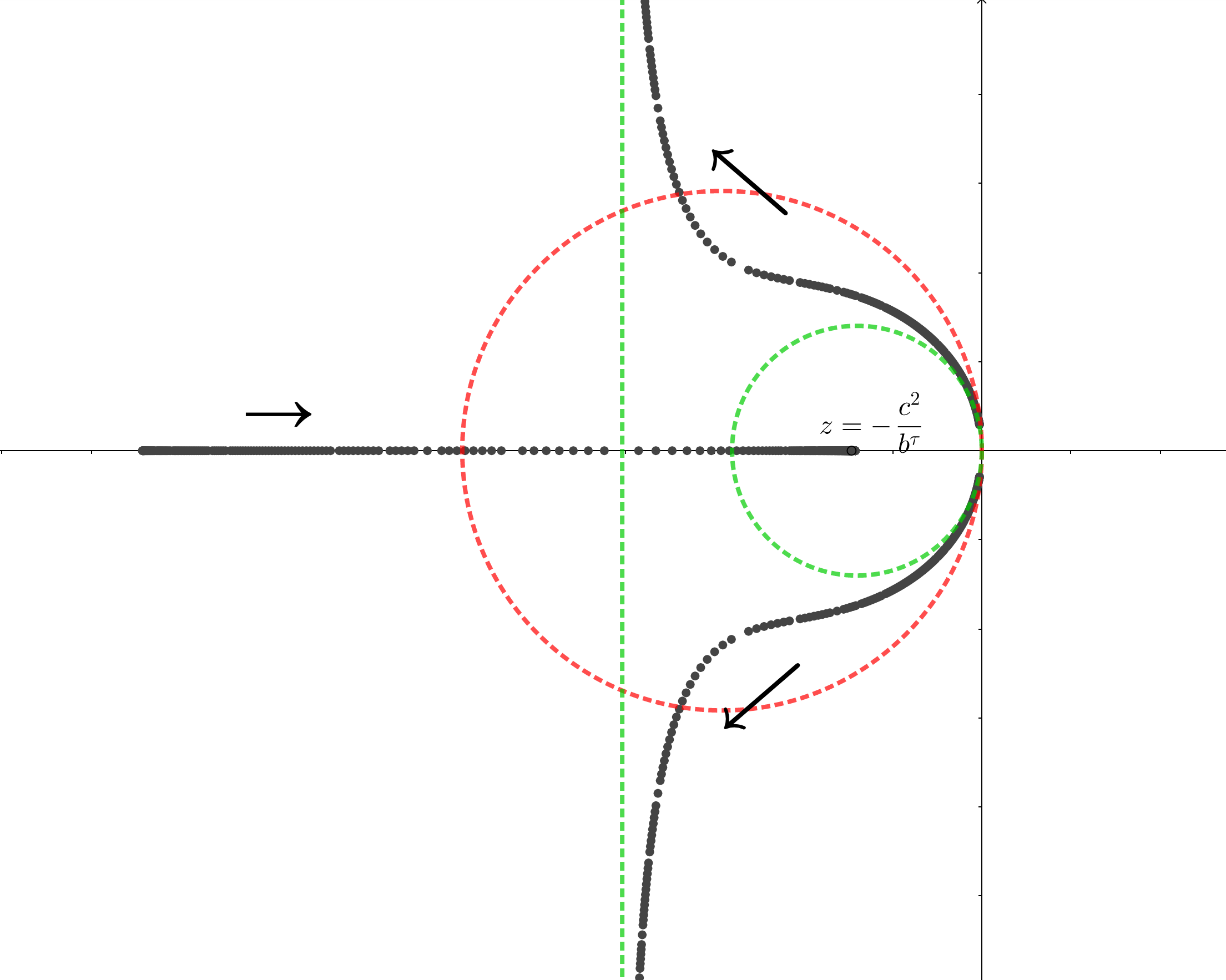
Refer to caption
Figure 2: Graphical representation of σp​(𝒜τ)\sigma_{p}(\mathcal{A}^{\tau}) and σc​(𝒜τ)\sigma_{c}(\mathcal{A}^{\tau}) for a τ=τ0∈(0,1]\tau=\tau_{0}\in(0,1] fixed: the circle in red is the same as in Figure 1 while the circle in green is centered at (−c2bτ,0)\left(-\frac{c^{2}}{b^{\tau}},0\right) and has radius r=c2bτ.r=\frac{c^{2}}{b^{\tau}}. The shape of the eigenvalues is represented by the curve of black dots. The green vertical line is given by x=−γτ2​τx=-\frac{\gamma^{\tau}}{2\tau} (see Theorem 2.4). The asymptotic behavior of the eigenvalues is exactly as we described in Theorem 2.4: as nn becomes large, two branches of the eigenvalues have their respective real parts converging to −γτ2​τ-\frac{\gamma^{\tau}}{2\tau} while their imaginary parts split into ±∞\pm\infty, and the other branch converges to the continuous spectrum, which in this case is given by the single point z=−c2bτ.z=-\frac{c^{2}}{b^{\tau}}.
Refer to caption
Figure 3: Graphical representation of σp​(𝒜τ)\sigma_{p}(\mathcal{A}^{\tau}) and σc​(𝒜τ)\sigma_{c}(\mathcal{A}^{\tau}) for a τ=τ0/10.\tau=\tau_{0}/10.
Refer to caption
Figure 4: Graphical representation of σp​(𝒜τ)\sigma_{p}(\mathcal{A}^{\tau}) and σc​(𝒜τ)\sigma_{c}(\mathcal{A}^{\tau}) for a τ=τ0/100:\tau=\tau_{0}/100: It is important to observe how the “vertical” spectrum escapes to  −∞-\infty as τ\tau becomes small.

The remaining part of the paper is devoted to the proofs of the main results.

3 Proofs

3.1 Proof of Theorem 2.2

Part I: Equi-boundedness of the groups

Let uτu^{\tau} be the solution for (2.1) and consider the energy functional Eτ​(t)E^{\tau}(t) defined as

Eτ​(t)=E0τ​(t)+E1τ​(t),E^{\tau}(t)=E_{0}^{\tau}(t)+E_{1}^{\tau}(t),

where

E0τ​(t)=α2​‖utτ​(t)‖22+c22​‖A1/2​uτ​(t)‖22E_{0}^{\tau}(t)=\dfrac{\alpha}{2}\|u^{\tau}_{t}(t)\|_{2}^{2}+\dfrac{c^{2}}{2}\|A^{1/2}u^{\tau}(t)\|_{2}^{2} (3.1)

and

E1τ​(t)=bτ2​‖A1/2​(utτ​(t)+c2bτ​uτ​(t))‖22+τ2​‖ut​tτ​(t)+c2bτ​utτ​(t)‖22+c2​γτ2​bτ​‖utτ​(t)‖22.E_{1}^{\tau}(t)=\dfrac{b^{\tau}}{2}\left\|A^{1/2}\left(u^{\tau}_{t}(t)+\dfrac{c^{2}}{b^{\tau}}u^{\tau}(t)\right)\right\|_{2}^{2}+\dfrac{\tau}{2}\left\|u^{\tau}_{tt}(t)+\dfrac{c^{2}}{b^{\tau}}u^{\tau}_{t}(t)\right\|_{2}^{2}+\dfrac{c^{2}\gamma^{\tau}}{2b^{\tau}}\|u^{\tau}_{t}(t)\|_{2}^{2}. (3.2)

The following differential identity can be derived for the functional E1τ​(t)E_{1}^{\tau}(t) :

dd​t​E1τ​(t)+γτ​‖ut​tτ​(t)‖22=0,\dfrac{d}{dt}E_{1}^{\tau}(t)+\gamma^{\tau}\|u^{\tau}_{tt}(t)\|_{2}^{2}=0, (3.3)

where γτ=α−c2​τ​(bτ)−1\gamma^{\tau}=\alpha-c^{2}\tau(b^{\tau})^{-1}. The proof of (3.3) follows along the same lines as in Lemma 3.1 [19] . The equality is derived first for smooth solution and then extended by density to the “energy” level solutions. For readers convenience the details of the derivation are given in the Appendix. Moreover, for each fixed value of τ>0,\tau>0, the authors in [19] establish exponential decay (with decay rates depending on τ\tau) provided γτ>0\gamma^{\tau}>0.

We aim to prove that the family of semigroups ℱ\mathcal{F} is equi-bounded in τ.\tau. In other words, there exists τ0\tau_{0} small enough such that if we consider τ∈(0,τ0],\tau\in(0,\tau_{0}], we can provide an uniform (in τ\tau) bound for the norm of the solutions in (ℍ0,∥⋅∥τ,0)=ℍ0τ(\mathbb{H}_{0},\|\cdot\|_{\tau,0})=\mathbb{H}_{0}^{\tau}. To achieve this, we establish first topological equivalence of energy function with respect to the topology defined on ℍ0τ\mathbb{H}_{0}^{\tau}. This is given in the lemma to follow.

Lemma 3.1.

Let U0∈ℍ0U_{0}\in\mathbb{H}_{0} and define τ0≡inf{c>0;γτ>0for allτ∈(0,c]}>0\tau_{0}\equiv\inf\{c>0;\gamma^{\tau}>0\ \mbox{for all}\ \tau\in(0,c]\}>0. Then there exist k=k⁡(τ0),K=K⁡(τ0)>0k=k(\tau_{0}),K=K(\tau_{0})>0 such that

k​‖Tτ​(t)​U0‖τ,02⩽Eτ​(t)⩽K​‖Tτ​(t)​U0‖τ,02,τ∈(0,τ0]k\|T^{\tau}(t)U_{0}\|^{2}_{\tau,0}\leqslant E^{\tau}(t)\leqslant K\|T^{\tau}(t)U_{0}\|^{2}_{\tau,0},\ \tau\in\left(0,\tau_{0}\right] (3.4)

for all t⩾0.t\geqslant 0.

Proof.

We begin with the second inequality-as an easier one. In order to get it, we observe that from (3.2) we have11 1 we have omitted the obvious dependence on t.t.:

Eτ​(t)=bτ2​‖A1/2​(utτ+c2bτ​uτ)‖22+τ2​‖ut​tτ+c2bτ​utτ‖22+(c2​γτ2​bτ+α2)​‖utτ‖22+c22​‖A1/2​uτ‖22\displaystyle E^{\tau}(t)=\dfrac{b^{\tau}}{2}\left\|A^{1/2}\left(u^{\tau}_{t}+\dfrac{c^{2}}{b^{\tau}}u^{\tau}\right)\right\|_{2}^{2}+\dfrac{\tau}{2}\left\|u^{\tau}_{tt}+\dfrac{c^{2}}{b^{\tau}}u^{\tau}_{t}\right\|_{2}^{2}+\left(\dfrac{c^{2}\gamma^{\tau}}{2b^{\tau}}+\frac{\alpha}{2}\right)\|u^{\tau}_{t}\|_{2}^{2}+\dfrac{c^{2}}{2}\|A^{1/2}u^{\tau}\|_{2}^{2}
⩽(bτ+c22)​‖A1/2​utτ‖22+c22​(2+c2bτ)​‖A1/2​uτ‖22+c22​bτ​(τ+c2​τbτ+α​bτc2+γτ)​‖utτ‖22+τ2​(1+c2bτ)​‖ut​tτ‖22\displaystyle\leqslant\left(\dfrac{b^{\tau}+c^{2}}{2}\right)\|A^{1/2}u_{t}^{\tau}\|_{2}^{2}+\dfrac{c^{2}}{2}\left(2+\dfrac{c^{2}}{b^{\tau}}\right)\|A^{1/2}u^{\tau}\|_{2}^{2}+\dfrac{c^{2}}{2b^{\tau}}\left(\tau+\dfrac{c^{2}\tau}{b^{\tau}}+\dfrac{\alpha b^{\tau}}{c^{2}}+\gamma^{\tau}\right)\|u_{t}^{\tau}\|_{2}^{2}+\dfrac{\tau}{2}\left(1+\dfrac{c^{2}}{b^{\tau}}\right)\|u_{tt}^{\tau}\|_{2}^{2}
⩽c22​(2+c2bτ)​‖A1/2​uτ‖22+c22​bτ​[C∗​(τ+c2​τbτ+γτ)+(α​C∗+bτ)​bτc2+bτ]​‖A1/2​utτ‖22+τ2​(1+c2bτ)​‖ut​tτ‖22\displaystyle\leqslant\dfrac{c^{2}}{2}\left(2+\dfrac{c^{2}}{b^{\tau}}\right)\|A^{1/2}u^{\tau}\|_{2}^{2}+\dfrac{c^{2}}{2b^{\tau}}\left[C^{\ast}\left(\tau+\dfrac{c^{2}\tau}{b^{\tau}}+\gamma^{\tau}\right)+\dfrac{(\alpha C^{\ast}+b^{\tau})b^{\tau}}{c^{2}}+b^{\tau}\right]\|A^{1/2}u_{t}^{\tau}\|_{2}^{2}+\dfrac{\tau}{2}\left(1+\dfrac{c^{2}}{b^{\tau}}\right)\|u_{tt}^{\tau}\|_{2}^{2}
⩽c22​(2+c2δ)​‖A1/2​uτ‖22+c22​δ​[C∗​(τ0+c2​τ0δ+γτ0)+(α​C∗+δ)​δc2+δ]​‖A1/2​utτ‖22+τ2​(1+c2δ)​‖ut​tτ‖22\displaystyle\leqslant\dfrac{c^{2}}{2}\left(2+\dfrac{c^{2}}{\delta}\right)\|A^{1/2}u^{\tau}\|_{2}^{2}+\dfrac{c^{2}}{2\delta}\left[\!C^{\ast}\!\!\left(\tau_{0}+\dfrac{c^{2}\tau_{0}}{\delta}+\gamma^{\tau_{0}}\right)+\dfrac{(\alpha C^{\ast}+\delta)\delta}{c^{2}}+\delta\right]\|A^{1/2}u_{t}^{\tau}\|_{2}^{2}+\dfrac{\tau}{2}\left(1+\dfrac{c^{2}}{\delta}\right)\|u_{tt}^{\tau}\|_{2}^{2}
⩽max⁡{c22​(2+c2δ);c22​δ​[C∗​(τ0+c2​τ0δ+γτ0)+(α​C∗+δ)​δc2+δ];12+c22​δ}​‖Uτ​(t)‖τ,02,\displaystyle\leqslant\max\left\{\dfrac{c^{2}}{2}\left(2+\dfrac{c^{2}}{\delta}\right);\dfrac{c^{2}}{2\delta}\left[\!C^{\ast}\!\!\left(\tau_{0}+\dfrac{c^{2}\tau_{0}}{\delta}+\gamma^{\tau_{0}}\right)+\dfrac{(\alpha C^{\ast}+\delta)\delta}{c^{2}}+\delta\right];\dfrac{1}{2}+\dfrac{c^{2}}{2\delta}\right\}\|U^{\tau}(t)\|^{2}_{\tau,0},
22 2 we have omitted the obvious dependence on t.t.

where C∗=C∗​(n,Ω)C^{\ast}=C^{\ast}(n,\Omega) is the constant that appears in Poincaré’s Inequality.

Now the second inequality in (3.4) follows after we define

K⁡(τ0)≡max⁡{c22​(2+c2δ);c22​δ​[C∗​(τ0+c2​τ0δ+γτ0)+(α​C∗+δ)​δc2+δ];12+c22​δ}.K(\tau_{0})\equiv\max\left\{\dfrac{c^{2}}{2}\left(2+\dfrac{c^{2}}{\delta}\right);\dfrac{c^{2}}{2\delta}\left[\!C^{\ast}\!\!\left(\tau_{0}+\dfrac{c^{2}\tau_{0}}{\delta}+\gamma^{\tau_{0}}\right)+\dfrac{(\alpha C^{\ast}+\delta)\delta}{c^{2}}+\delta\right];\dfrac{1}{2}+\dfrac{c^{2}}{2\delta}\right\}. (3.5)

For the first inequality, fix ε>0\varepsilon>0 to be determined later. Peter-Paul inequality then implies that

−c2​ε​‖A1/2​utτ‖222−c2​‖A1/2​uτ‖222​ε⩽c2​(A1/2​uτ,A1/2​utτ)and−ε​τ​c22​bτ​‖ut​tτ‖22−τ​c22​ε​bτ​‖utτ‖22⩽τ​c2bτ​(ut​tτ,utτ).-\frac{c^{2}\varepsilon\|A^{1/2}u^{\tau}_{t}\|_{2}^{2}}{2}-\frac{c^{2}\|A^{1/2}u^{\tau}\|_{2}^{2}}{2\varepsilon}\leqslant c^{2}(A^{1/2}u^{\tau},A^{1/2}u^{\tau}_{t})\ \ \mbox{and}\ -\frac{\varepsilon\tau c^{2}}{2b^{\tau}}\|u^{\tau}_{tt}\|_{2}^{2}-\frac{\tau c^{2}}{2\varepsilon b^{\tau}}\|u^{\tau}_{t}\|_{2}^{2}\leqslant\frac{\tau c^{2}}{b^{\tau}}(u^{\tau}_{tt},u^{\tau}_{t}). (3.6)

Then we have

Eτ​(t)=bτ2​‖A1/2​(utτ+c2bτ​uτ)‖22+τ2​‖ut​tτ+c2bτ​utτ‖22+(c2​γτ2​bτ+α2)​‖utτ‖22+c22​‖A1/2​uτ‖22\displaystyle E^{\tau}(t)=\dfrac{b^{\tau}}{2}\left\|A^{1/2}\left(u^{\tau}_{t}+\dfrac{c^{2}}{b^{\tau}}u^{\tau}\right)\right\|_{2}^{2}+\dfrac{\tau}{2}\left\|u^{\tau}_{tt}+\dfrac{c^{2}}{b^{\tau}}u^{\tau}_{t}\right\|_{2}^{2}+\left(\dfrac{c^{2}\gamma^{\tau}}{2b^{\tau}}+\frac{\alpha}{2}\right)\|u^{\tau}_{t}\|_{2}^{2}+\dfrac{c^{2}}{2}\|A^{1/2}u^{\tau}\|_{2}^{2}
=c22​(+c2bτ)​‖A1/2​uτ‖22+bτ2​‖A1/2​utτ‖22+c2​(A1/2​uτ,A1/2​utτ)+τ2​‖ut​tτ‖22+α2​(+c2bτ)​‖utτ‖22+τ​c2bτ​(ut​tτ,utτ)\displaystyle=\dfrac{c^{2}}{2}\!\left(\!1\!+\!\dfrac{c^{2}}{b^{\tau}}\right)\!\!\|A^{1/2}u^{\tau}\|_{2}^{2}+\dfrac{b^{\tau}}{2}\|A^{1/2}u^{\tau}_{t}\|_{2}^{2}+c^{2}(A^{1/2}u^{\tau},A^{1/2}u_{t}^{\tau})+\dfrac{\tau}{2}\|u_{tt}^{\tau}\|_{2}^{2}+\dfrac{\alpha}{2}\!\!\left(1\!+\!\frac{c^{2}}{b^{\tau}}\!\right)\!\!\|u^{\tau}_{t}\|_{2}^{2}+\dfrac{\tau c^{2}}{b^{\tau}}(u^{\tau}_{tt},u^{\tau}_{t})
⩾c22​(+c2bτ−1ε)​‖A1/2​uτ‖22+(bτ2−c2​ε2)​‖A1/2​utτ‖22+τ2​(1−c2​εbτ)​‖ut​tτ‖22+(α2​(+c2bτ)−τ​c22​ε​bτ)​‖utτ‖22,\displaystyle\geqslant\dfrac{c^{2}}{2}\!\left(\!1\!+\!\dfrac{c^{2}}{b^{\tau}}-\dfrac{1}{\varepsilon}\right)\!\!\|A^{1/2}u^{\tau}\|_{2}^{2}+\left(\dfrac{b^{\tau}}{2}-\frac{c^{2}\varepsilon}{2}\right)\|A^{1/2}u^{\tau}_{t}\|_{2}^{2}+\dfrac{\tau}{2}\left(1-\dfrac{c^{2}\varepsilon}{b^{\tau}}\right)\|u_{tt}^{\tau}\|_{2}^{2}+\left(\dfrac{\alpha}{2}\!\!\left(1\!+\!\frac{c^{2}}{b^{\tau}}\!\right)-\dfrac{\tau c^{2}}{2\varepsilon b^{\tau}}\right)\|u^{\tau}_{t}\|_{2}^{2},

Pick an ε>0\varepsilon>0 such that bτbτ+c2<ε<bτc2\dfrac{b^{\tau}}{b^{\tau}+c^{2}}<\varepsilon<\dfrac{b^{\tau}}{c^{2}} and observe that

bτ2−c2​ε2>0\dfrac{b^{\tau}}{2}-\dfrac{c^{2}\varepsilon}{2}>0 and c22​(c221)−c22​ε=c22​(c2bτ+1−1ε)>0\dfrac{c^{2}}{2}\bigg(\dfrac{c^{2}}{2}_{1}\bigg)-\dfrac{c^{2}}{2\varepsilon}=\dfrac{c^{2}}{2}\bigg(\dfrac{c^{2}}{b^{\tau}}+1-\dfrac{1}{\varepsilon}\bigg)>0

and similarly

τ2−ε​τ​c22​bτ>0 and α2​(c2bτ+1)−τ​c22​ε​bτ=α2​(c2bτ+1−1ε)=γτ2​(c2bτ+1)+τ​c22​bτ​(c2bτ+1−1ε)>0.\text{$\dfrac{\tau}{2}-\dfrac{\varepsilon\tau c^{2}}{2b^{\tau}}>0$ and $\dfrac{\alpha}{2}\bigg(\dfrac{c^{2}}{b^{\tau}}+1\bigg)-\dfrac{\tau c^{2}}{2\varepsilon b^{\tau}}=\dfrac{\alpha}{2}\bigg(\dfrac{c^{2}}{b^{\tau}}+1-\dfrac{1}{\varepsilon}\bigg)=\dfrac{\gamma^{\tau}}{2}\bigg(\dfrac{c^{2}}{b^{\tau}}+1\bigg)+\dfrac{\tau c^{2}}{2b^{\tau}}\bigg(\dfrac{c^{2}}{b^{\tau}}+1-\dfrac{1}{\varepsilon}\bigg)>0$}.

Hence, picking

ε=2​bτbτ+2​c2\varepsilon=\dfrac{2b^{\tau}}{b^{\tau}+2c^{2}}

and continuing the lower bound estimate of Eτ​(t)E^{\tau}(t) we have

Eτ​(t)\displaystyle E^{\tau}(t) ⩾c22​(+c2bτ−1ε)​‖A1/2​uτ‖22+(bτ2−c2​ε2)​‖A1/2​utτ‖22+τ2​(1−c2​εbτ)​‖ut​tτ‖22\displaystyle\geqslant\dfrac{c^{2}}{2}\!\left(\!1\!+\!\dfrac{c^{2}}{b^{\tau}}-\dfrac{1}{\varepsilon}\right)\!\!\|A^{1/2}u^{\tau}\|_{2}^{2}+\left(\dfrac{b^{\tau}}{2}-\frac{c^{2}\varepsilon}{2}\right)\|A^{1/2}u^{\tau}_{t}\|_{2}^{2}+\dfrac{\tau}{2}\left(1-\dfrac{c^{2}\varepsilon}{b^{\tau}}\right)\|u_{tt}^{\tau}\|_{2}^{2}
⩾c24​‖A1/2​uτ‖22+δ2(4+τ0)​c2+2​δ​‖A1/2​utτ‖22+τ​δ2​δ+(4+τ0)​c2​‖ut​tτ‖22\displaystyle\geqslant\dfrac{c^{2}}{4}\|A^{1/2}u^{\tau}\|_{2}^{2}+\dfrac{\delta^{2}}{(4+\tau_{0})c^{2}+2\delta}\|A^{1/2}u^{\tau}_{t}\|_{2}^{2}+\dfrac{\tau\delta}{2\delta+(4+\tau_{0})c^{2}}\|u_{tt}^{\tau}\|_{2}^{2}
⩾min⁡{c24;δ2(4+τ0)​c2+2​δ;δ2​δ+(4+τ0)​c2}​‖Uτ​(t)‖τ,02.\displaystyle\geqslant\min\left\{\dfrac{c^{2}}{4};\dfrac{\delta^{2}}{(4+\tau_{0})c^{2}+2\delta};\dfrac{\delta}{2\delta+(4+\tau_{0})c^{2}}\right\}\|U^{\tau}(t)\|^{2}_{\tau,0}.

where we have used

c22​(1+c2bτ−1ε)=c24,\dfrac{c^{2}}{2}\left(1+\dfrac{c^{2}}{b^{\tau}}-\dfrac{1}{\varepsilon}\right)=\dfrac{c^{2}}{4},
bτ2−c2​ε2=(bτ)24​c2+2​bτ⩾δ2(4+τ0)​c2+2​δ\displaystyle\dfrac{b^{\tau}}{2}-\frac{c^{2}\varepsilon}{2}=\dfrac{(b^{\tau})^{2}}{4c^{2}+2b^{\tau}}\geqslant\dfrac{\delta^{2}}{(4+\tau_{0})c^{2}+2\delta}

and similarly

τ2​(1−c2​εbτ)=τ​bτ2​bτ+4​c2⩾τ​δ2​δ+(4+τ0)​c2.\dfrac{\tau}{2}\left(1-\dfrac{c^{2}\varepsilon}{b^{\tau}}\right)=\dfrac{\tau b^{\tau}}{2b^{\tau}+4c^{2}}\geqslant\dfrac{\tau\delta}{2\delta+(4+\tau_{0})c^{2}}.

Setting

k⁡(τ0)≡min⁡{c24;δ2(4+τ0)​c2+2​δ;δ2​δ+(4+τ0)​c2}k(\tau_{0})\equiv\min\left\{\dfrac{c^{2}}{4};\dfrac{\delta^{2}}{(4+\tau_{0})c^{2}+2\delta};\dfrac{\delta}{2\delta+(4+\tau_{0})c^{2}}\right\} (3.7)

gives the first part of the inequality in Lemma 3.1. This completes the proof of the Lemma.

∎

Lemma 3.1 along with the identity (3.3) imply the equi-boundedness of the family ℱ\mathcal{F}. Indeed,

Lemma 3.2.

Let U0∈ℍ0.U_{0}\in\mathbb{H}_{0}. For given kk in (3.7) and KK in (3.5), there exists a constant L1>0L_{1}>0 (independent on τ∈(0,τ0)\tau\in(0,\tau_{0})) such that

‖Tτ​(t)​U0‖τ,02⩽1k​Eτ​(t)⩽L1​Kk​‖U0‖τ,02.\|T^{\tau}(t)U_{0}\|^{2}_{\tau,0}\leqslant\dfrac{1}{k}E^{\tau}(t)\leqslant\dfrac{L_{1}K}{k}\|U_{0}\|^{2}_{\tau,0}.
Proof.

We work with sufficiently smooth solutions guaranteed by the well-posedness-regularity theory. The final estimates are obtained via density.

Taking the L2−L^{2}-inner product of (2.1) with utτu^{\tau}_{t} we obtain

bτ​‖A1/2​utτ​(t)‖22=τ​‖ut​tτ​(t)‖22−dd​t​[α2​‖utτ‖22+c22​‖A1/2​uτ‖22+τ⁡(ut​tτ,utτ)].b^{\tau}\|A^{1/2}u^{\tau}_{t}(t)\|_{2}^{2}=\tau\|u^{\tau}_{tt}(t)\|_{2}^{2}-\dfrac{d}{dt}\left[\dfrac{\alpha}{2}\|u^{\tau}_{t}\|_{2}^{2}+\dfrac{c^{2}}{2}\|A^{1/2}u^{\tau}\|_{2}^{2}+\tau(u^{\tau}_{tt},u^{\tau}_{t})\right]. (3.8)

Multiplying (3.8) by γτ\gamma^{\tau} with using (3.1) gives

γτ​bτ​‖A1/2​utτ​(t)‖22=γτ​τ​‖ut​tτ​(t)‖22−γτ​dd​t​E0τ​(t)−γτ​τ​dd​t​(ut​tτ,utτ)\gamma^{\tau}b^{\tau}\|A^{1/2}u^{\tau}_{t}(t)\|_{2}^{2}=\gamma^{\tau}\tau\|u^{\tau}_{tt}(t)\|_{2}^{2}-\gamma^{\tau}\dfrac{d}{dt}E^{\tau}_{0}(t)-\gamma^{\tau}\tau\dfrac{d}{dt}(u^{\tau}_{tt},u^{\tau}_{t}) (3.9)

Combine (3.9) with the identity (3.3) we obtain

dd​t​E1τ​(t)+γτ​dd​t​E0τ​(t)+bτ​γτ​‖A1/2​utτ​(t)‖22=γτ​(τ−1)​‖ut​tτ​(t)‖22−γτ​τ​dd​t​(ut​tτ,utτ).\dfrac{d}{dt}E_{1}^{\tau}(t)+\gamma^{\tau}\dfrac{d}{dt}E^{\tau}_{0}(t)+b^{\tau}\gamma^{\tau}\|A^{1/2}u^{\tau}_{t}(t)\|_{2}^{2}=\gamma^{\tau}(\tau-1)\|u^{\tau}_{tt}(t)\|^{2}_{2}-\gamma^{\tau}\tau\dfrac{d}{dt}(u^{\tau}_{tt},u^{\tau}_{t}). (3.10)

Since τ\tau is very small and we assume 0<τ<1,0<\tau<1, we have γτ​(τ−1)​‖ut​tτ​(t)‖22<0\gamma^{\tau}(\tau-1)\|u^{\tau}_{tt}(t)\|^{2}_{2}<0 for all t∈[0,T].t\in[0,T].

Then integrating w.r.t. time from 00 to tt we have

E1τ(t)+γτE0τ(t)+γτbτ∫0t∥A1/2utτ(s)∥22ds⩽E1τ(0)+γτE0τ(0)+γττ(ut​tτ,utτ)|0t.E_{1}^{\tau}(t)+\gamma^{\tau}E^{\tau}_{0}(t)+\gamma^{\tau}b^{\tau}\int_{0}^{t}\|A^{1/2}u^{\tau}_{t}(s)\|_{2}^{2}ds\leqslant E_{1}^{\tau}(0)+\gamma^{\tau}E^{\tau}_{0}(0)+\gamma^{\tau}\tau(u^{\tau}_{tt},u^{\tau}_{t})\big\rvert_{0}^{t}. (3.11)

From (3.3), we have E1τ​(t)⩽E1τ​(0)E_{1}^{\tau}(t)\leqslant E_{1}^{\tau}(0) and notice that

τ(ut​tτ,utτ)|0t\displaystyle\tau(u^{\tau}_{tt},u^{\tau}_{t})\big\rvert_{0}^{t} =τ⁡(ut​tτ​(t),utτ​(t))−τ⁡(u2,u1)\displaystyle=\tau(u^{\tau}_{tt}(t),u^{\tau}_{t}(t))-\tau(u_{2},u_{1})
⩽τ2​‖ut​tτ​(t)‖22+τ2​‖utτ​(t)‖22+τ2​‖u2‖22+τ2​‖u1‖22\displaystyle\leqslant\dfrac{\tau}{2}\|u^{\tau}_{tt}(t)\|_{2}^{2}+\dfrac{\tau}{2}\|u_{t}^{\tau}(t)\|_{2}^{2}+\dfrac{\tau}{2}\|u_{2}\|_{2}^{2}+\dfrac{\tau}{2}\|u_{1}\|_{2}^{2}
⩽(1+τ​bα​c2)​[E1τ​(t)+E1τ​(0)]⩽2​(α​c2+τ​bα​c2)​E1τ​(0).\displaystyle\leqslant\bigg(1+\dfrac{\tau b}{\alpha c^{2}}\bigg)\bigg[E_{1}^{\tau}(t)+E_{1}^{\tau}(0)\bigg]\leqslant 2\bigg(\dfrac{\alpha c^{2}+\tau b}{\alpha c^{2}}\bigg)E_{1}^{\tau}(0).

Then

E1τ​(t)+γτ​E0τ​(t)+γτ​bτ​∫0t‖A1/2​utτ​(s)‖22​𝑑s⩽E1τ​(0)+γτ​E0τ​(0)+2​γτ​(α​c2+τ​bτα​c2)​E1τ​(0).E_{1}^{\tau}(t)+\gamma^{\tau}E^{\tau}_{0}(t)+\gamma^{\tau}b^{\tau}\int_{0}^{t}\|A^{1/2}u^{\tau}_{t}(s)\|_{2}^{2}ds\leqslant E_{1}^{\tau}(0)+\gamma^{\tau}E^{\tau}_{0}(0)+2\gamma^{\tau}\bigg(\dfrac{\alpha c^{2}+\tau b^{\tau}}{\alpha c^{2}}\bigg)E_{1}^{\tau}(0).
E1τ​(t)+γτ​E0τ​(t)⩽max⁡{α​c2+2​γτ​(α​c2+τ​bτ)α​c2,γτ}​Eτ​(0)E_{1}^{\tau}(t)+\gamma^{\tau}E^{\tau}_{0}(t)\leqslant\max\biggl\{\dfrac{\alpha c^{2}+2\gamma^{\tau}(\alpha c^{2}+\tau b^{\tau})}{\alpha c^{2}},\gamma^{\tau}\biggr\}E^{\tau}(0)

Therefore

Eτ​(t)⩽max⁡{α​c2+2​γτ0​α​c2+τ​bτα​c2,γτ0}min⁡{1,γτ0}​Eτ​(0)=L1​Eτ​(0)E^{\tau}(t)\leqslant\dfrac{\max\biggl\{\dfrac{\alpha c^{2}+2\gamma^{\tau_{0}}\alpha c^{2}+\tau b^{\tau}}{\alpha c^{2}},\gamma^{\tau_{0}}\biggr\}}{\min\{1,\gamma^{\tau_{0}}\}}E^{\tau}(0)=L_{1}E^{\tau}(0) (3.12)

This means that the total energy Eτ​(t)E^{\tau}(t) is bounded in time by the initial total energy. Thus the proof is obtained. ∎

From Lemma 3.2 we conclude

Corollary 3.3.

There exists a constant M>0M>0 (independent on τ∈(0,τ0)\tau\in(0,\tau_{0})) such that

‖Tτ​(t)‖ℒ⁡(ℍ0τ)⩽M,∀t>0.\|T^{\tau}(t)\|_{\mathcal{L}(\mathbb{H}^{\tau}_{0})}\leqslant M,\forall t>0. (3.13)

Part II: Uniform (in τ\tau) decay rates

In order to prove the uniformity of the decay rates we use the Pazy-Datko Theorem. The first step consists of showing the the map t↦‖Tτ​(t)​U0‖τ,02t\mapsto\|T^{\tau}(t)U_{0}\|^{2}_{\tau,0} belongs to L1​(0,∞,ℍ0).L^{1}(0,\infty;\mathbb{H}_{0}). This is the statement of the next Lemma.

Lemma 3.4.

There exists K¯>0\overline{K}>0 independent on τ\tau such that

∫0∞‖Tτ​(s)​U0‖τ,02​𝑑s⩽K¯​‖U0‖τ,02<∞.\int_{0}^{\infty}\|T^{\tau}(s)U_{0}\|^{2}_{\tau,0}ds\leqslant\overline{K}\|U_{0}\|^{2}_{\tau,0}<\infty. (3.14)
Proof.

Multiplying the identity (3.3) by 2​τ2\tau gives

2​τ​dd​t​E1τ​(t)+2​τ​γτ​‖ut​tτ​(t)‖22=02\tau\dfrac{d}{dt}E_{1}^{\tau}(t)+2\tau\gamma^{\tau}\|u^{\tau}_{tt}(t)\|_{2}^{2}=0 (3.15)

Multiply (3.8) by γτ\gamma^{\tau} we have

γτ​bτ​‖A1/2​utτ​(t)‖22=γτ​τ​‖ut​tτ​(t)‖22−γτ​dd​t​E0τ​(t)+γτ​τ​dd​t​(ut​tτ,utτ)\gamma^{\tau}b^{\tau}\|A^{1/2}u^{\tau}_{t}(t)\|_{2}^{2}=\gamma^{\tau}\tau\|u^{\tau}_{tt}(t)\|_{2}^{2}-\gamma^{\tau}\dfrac{d}{dt}E^{\tau}_{0}(t)+\gamma^{\tau}\tau\dfrac{d}{dt}(u^{\tau}_{tt},u^{\tau}_{t}) (3.16)

With (3.15) and (3.16) we get

2​τ​dd​t​E1τ​(t)+γτ​dd​t​E0τ​(t)+τ​γτ​‖ut​tτ​(t)‖22+bτ​γτ​‖A1/2​utτ​(t)‖22=−γτ​τ​dd​t​(ut​tτ,utτ).2\tau\dfrac{d}{dt}E_{1}^{\tau}(t)+\gamma^{\tau}\dfrac{d}{dt}E^{\tau}_{0}(t)+\tau\gamma^{\tau}\|u^{\tau}_{tt}(t)\|^{2}_{2}+b^{\tau}\gamma^{\tau}\|A^{1/2}u^{\tau}_{t}(t)\|_{2}^{2}=-\gamma^{\tau}\tau\dfrac{d}{dt}(u^{\tau}_{tt},u^{\tau}_{t}). (3.17)

Then integrating w.r.t. time from 00 to tt we have

2τE1τ(t)+γτE0τ(t)+γτ∫0t[τ∥ut​tτ(s)∥22+bτ∥A1/2utτ(s)∥22]ds=2τE1τ(0)+γτE0τ(0)−γττ(ut​tτ,utτ)|0t.2\tau E_{1}^{\tau}(t)+\gamma^{\tau}E^{\tau}_{0}(t)+\gamma^{\tau}\int_{0}^{t}\left[\tau\|u^{\tau}_{tt}(s)\|^{2}_{2}+b^{\tau}\|A^{1/2}u^{\tau}_{t}(s)\|_{2}^{2}\right]ds=2\tau E_{1}^{\tau}(0)+\gamma^{\tau}E^{\tau}_{0}(0)-\gamma^{\tau}\tau(u^{\tau}_{tt},u^{\tau}_{t})\big\rvert_{0}^{t}. (3.18)

Notice that from Lemma 3.2 we have

τ(ut​tτ,utτ)|0t⩽(1+τ0)(∥Tτ(t)U0∥τ2+∥U0∥τ2)⩽(1+τ0)​(L1​K+k)k∥U0∥τ2.\tau(u^{\tau}_{tt},u^{\tau}_{t})\big\rvert_{0}^{t}\leqslant(1+\tau_{0})\left(\|T^{\tau}(t)U_{0}\|_{\tau}^{2}+\|U_{0}\|_{\tau}^{2}\right)\leqslant\dfrac{(1+\tau_{0})(L_{1}K+k)}{k}\|U_{0}\|_{\tau}^{2}.

Therefore,

∫0t[τ​‖ut​tτ​(s)‖22+bτ​‖A1/2​utτ​(s)‖22]​𝑑s\displaystyle\int_{0}^{t}\left[\tau\|u^{\tau}_{tt}(s)\|_{2}^{2}+b^{\tau}\|A^{1/2}u^{\tau}_{t}(s)\|_{2}^{2}\right]ds ⩽γτ​(1+τ0)​(L1​K+k)+(2​τ0+γτ)​L1​K​kk​γτ​‖U0‖τ,02\displaystyle\leqslant\dfrac{\gamma^{\tau}(1+\tau_{0})(L_{1}K+k)+(2\tau_{0}+\gamma^{\tau})L_{1}Kk}{k\gamma^{\tau}}\|U_{0}\|^{2}_{\tau,0}
⩽γτ0​(1+τ0)​(L1​K+k)+(2​τ0+γτ0)​L1​K​kk​γτ0​‖U0‖τ,02=M1​‖U0‖τ,02.\displaystyle\leqslant\dfrac{\gamma^{\tau_{0}}(1+\tau_{0})(L_{1}K+k)+(2\tau_{0}+\gamma^{\tau_{0}})L_{1}Kk}{k\gamma^{\tau_{0}}}\|U_{0}\|^{2}_{\tau,0}=M_{1}\|U_{0}\|^{2}_{\tau,0}. (3.19)

Similarly, taking the L2−L^{2}-inner product of (2.1) with uτu^{\tau} we have

bτ2dd​t∥A1/2uτ∥22+c2∥A1/2uτ(t)∥22=α∥utτ(t)∥22+dd​t[τ2∥utτ|∥22−τ(ut​tτ,uτ)−α(utτ,uτ)]\dfrac{b^{\tau}}{2}\dfrac{d}{dt}\|A^{1/2}u^{\tau}\|_{2}^{2}+c^{2}\|A^{1/2}u^{\tau}(t)\|_{2}^{2}=\alpha\|u^{\tau}_{t}(t)\|_{2}^{2}+\dfrac{d}{dt}\left[\dfrac{\tau}{2}\|u^{\tau}_{t}|\|_{2}^{2}-\tau(u^{\tau}_{tt},u^{\tau})-\alpha(u^{\tau}_{t},u^{\tau})\right] (3.20)

and integrating (3.20) w.r.t time from 00 to tt we have

bτ2​‖A1/2​uτ​(t)‖22\displaystyle\dfrac{b^{\tau}}{2}\|A^{1/2}u^{\tau}(t)\|_{2}^{2} +c2∫0t∥A1/2uτ(s)∥22ds\displaystyle+c^{2}\int_{0}^{t}\|A^{1/2}u^{\tau}(s)\|_{2}^{2}ds
=bτ2∥A1/2u0∥22+α∫0t∥utτ(s)∥22ds+[τ2∥utτ|∥22−τ(ut​tτ,uτ)−α(utτ,uτ)]|0t\displaystyle=\dfrac{b^{\tau}}{2}\|A^{1/2}u_{0}\|_{2}^{2}+\alpha\int_{0}^{t}\|u^{\tau}_{t}(s)\|_{2}^{2}ds+\left[\dfrac{\tau}{2}\|u^{\tau}_{t}|\|_{2}^{2}-\tau(u^{\tau}_{tt},u^{\tau})-\alpha(u^{\tau}_{t},u^{\tau})\right]\biggr\rvert_{0}^{t}
⩽bτ​‖U0‖τ,02+α​M1bτ​‖U0‖τ,02+[(α+τ0)​C∗+1]​(L1​K+k)k​‖U0‖τ,02\displaystyle\leqslant b^{\tau}\|U_{0}\|^{2}_{\tau,0}+\dfrac{\alpha M_{1}}{b^{\tau}}\|U_{0}\|^{2}_{\tau,0}+\dfrac{\big[(\alpha+\tau_{0})C^{\ast}+1\big](L_{1}K+k)}{k}\|U_{0}\|^{2}_{\tau,0}
=k​bτ+α​k​M1+bτ​[(α+τ0)​C∗+1]​(L1​K+k)bτ​k​‖U0‖τ,02\displaystyle=\dfrac{kb^{\tau}+\alpha kM_{1}+b^{\tau}\big[(\alpha+\tau_{0})C^{\ast}+1\big](L_{1}K+k)}{b^{\tau}k}\|U_{0}\|^{2}_{\tau,0}
⩽k​δ+α​k​M1+δ⁡[(α+τ0)​C∗+1]​(L1​K+k)δ​k​‖U0‖τ,02=M2​‖U0‖τ,02.\displaystyle\leqslant\dfrac{k\delta+\alpha kM_{1}+\delta\big[(\alpha+\tau_{0})C^{\ast}+1\big](L_{1}K+k)}{\delta k}\|U_{0}\|^{2}_{\tau,0}=M_{2}\|U_{0}\|^{2}_{\tau,0}. (3.21)

Hence, by (3.1) and (3.1) we get

∫0∞‖Tτ​(s)​U0‖τ2​𝑑s⩽M1+M21+δ+c2​‖U0‖τ2=M3​‖U0‖τ2<∞.\int_{0}^{\infty}\|T^{\tau}(s)U_{0}\|^{2}_{\tau}ds\leqslant\dfrac{M_{1}+M_{2}}{1+\delta+c^{2}}\|U_{0}\|^{2}_{\tau}=M_{3}\|U_{0}\|^{2}_{\tau}<\infty. (3.22)

Therefore, according to Theorem 4.1 ([29], p. 116) the rate ω\omega can be determined as follows: We first chose a number ρ\rho such that 0<ρ<M3−1,0<\rho<M_{3}^{-1}, then we define a number η0=M3​ρ−1\eta_{0}=M_{3}\rho^{-1} and choose another number η\eta such that η>η0.\eta>\eta_{0}. The rate is then given by

ω=−1η​log⁡(M3​ρ)>0,\omega=-\dfrac{1}{\eta}\log(M_{3}\rho)>0,

and is clearly independent on τ.\tau. The proof is thus completed. ∎

3.2 Proof of Theorem 2.3

(a) Well-posedness

The well-posedness follows directly from Theorem 1.4 in [18] and the fact that on the space ℍ1\mathbb{H}_{1} the standard sum norm ∥⋅∥\|\cdot\| and ∥⋅∥τ,1\|\cdot\|_{\tau,1} are equivalent for each τ∈(0,1]\tau\in(0,1].

(b) Equi-boundedness on ℍ1τ\mathbb{H}_{1}^{\tau} and uniform (in τ\tau) exponential stability

Let uτu^{\tau} be the solution for (2.1) and consider the energy functional ℰτ​(t)\mathcal{E}^{\tau}(t) defined as

ℰτ​(t)=Eτ​(t)+‖A​uτ​(t)‖22.\mathcal{E}^{\tau}(t)=E^{\tau}(t)+\|Au^{\tau}(t)\|_{2}^{2}. (3.23)

By Theorem 1.3 ([18]) the energy functional above (which is equivalent to the ‖(uτ,utτ,ut​tτ)‖\|(u^{\tau},u^{\tau}_{t},u^{\tau}_{tt})\| for all t⩾0t\geqslant 0) decays exponentially with time [for each fixed τ>0,\tau>0, provided γτ≡α−c2​τ​(bτ)−1>0\gamma^{\tau}\equiv\alpha-c^{2}\tau(b^{\tau})^{-1}>0.

As in the previous theorem, the equi-boundedness of the family ℱ1\mathcal{F}_{1} follows from the lemma:

Lemma 3.5.

Let U0∈ℍ1U_{0}\in\mathbb{H}_{1} and define τ0≡inf{c>0;γτ>0for allτ∈(0,c]}>0\tau_{0}\equiv\inf\{c>0;\gamma^{\tau}>0\ \mbox{for all}\ \tau\in(0,c]\}>0. Then there exist k1=k1​(τ0)k_{1}=k_{1}(\tau_{0}) and K1=K1​(τ0)K_{1}=K_{1}(\tau_{0}) such that

k1​‖Tτ​(t)​U0‖τ,12⩽ℰτ​(t)⩽K1​‖Tτ​(t)​U0‖τ,12,τ∈(0,τ0]k_{1}\|T^{\tau}(t)U_{0}\|^{2}_{\tau,1}\leqslant\mathcal{E}^{\tau}(t)\leqslant K_{1}\|T^{\tau}(t)U_{0}\|^{2}_{\tau,1},\ \tau\in\left(0,\tau_{0}\right]

for all t⩾0.t\geqslant 0.

The proof of Lemma 3.5 as well as the conclusion of the equi-boundedness in ℍ1\mathbb{H}_{1} capitalizes on the estimates already derived for ℍ0\mathbb{H}_{0}. We shall focus on additional terms which need to be estimated additionally.

Lemma 3.5 is obtained from Lemma 3.1 and the estimates already derived for the space ℍ0τ\mathbb{H}_{0}^{\tau} by adding the term ‖A​uτ​(t)‖22||Au^{\tau}(t)||^{2}_{2}. This gives the inequality stated in Lemma 3.5. Recall (3.12), we will obtain the apriori bound for ℰτ​(t)\mathcal{E}^{\tau}(t) from the relation

ℰτ​(t)=Eτ​(t)+‖A​uτ​(t)‖22≤L1​Eτ​(0)+supt≥0‖A​uτ​(t)‖22.\mathcal{E}^{\tau}(t)=E^{\tau}(t)+||Au^{\tau}(t)||^{2}_{2}\leq L_{1}E^{\tau}(0)+\sup_{t\geq 0}||Au^{\tau}(t)||^{2}_{2}.

To achieve the goal, the second term needs to be accounted for. To estimate the second term we employ the equality by taking the L2−L^{2}-inner product of (2.1) with the multiplier A​uτAu^{\tau} and integrating w.r.t time from 00 to tt

bτ2​‖A​uτ​(t)‖22\displaystyle\dfrac{b^{\tau}}{2}\|Au^{\tau}(t)\|_{2}^{2} +c2∫0t∥Auτ(s)∥22ds=bτ2∥Au0∥22\displaystyle+c^{2}\int_{0}^{t}\|Au^{\tau}(s)\|_{2}^{2}ds=\dfrac{b^{\tau}}{2}\|Au_{0}\|_{2}^{2}
+α∫0t∥A1/2utτ(s)∥22ds+[τ2∥A1/2utτ|∥22−τ(ut​tτ,Auτ)−α(utτ,Auτ)]|0t\displaystyle+\alpha\int_{0}^{t}\|A^{1/2}u^{\tau}_{t}(s)\|_{2}^{2}ds+\left[\dfrac{\tau}{2}\|A^{1/2}u^{\tau}_{t}|\|_{2}^{2}-\tau(u^{\tau}_{tt},Au^{\tau})-\alpha(u^{\tau}_{t},Au^{\tau})\right]\biggr\rvert_{0}^{t} (3.24)

and by using the already obtained estimates in ℍ0τ\mathbb{H}_{0}^{\tau}

(bτ−ε)2​‖A​uτ​(t)‖22+c2​∫0t‖A​uτ​(s)‖22​𝑑s\displaystyle\dfrac{(b^{\tau}-\varepsilon)}{2}\|Au^{\tau}(t)\|_{2}^{2}+c^{2}\int_{0}^{t}\|Au^{\tau}(s)\|_{2}^{2}ds ⩽bτ​‖U0‖τ,12+α​M​3​‖U0‖τ,12+(τ2+τ​Cε+α)​(K1+k1)k1​‖U0‖τ,12\displaystyle\leqslant b^{\tau}\|U_{0}\|^{2}_{\tau,1}+\alpha M3\|U_{0}\|^{2}_{\tau,1}+\dfrac{\big(\dfrac{\tau}{2}+\tau C_{\varepsilon}+\alpha\big)(K_{1}+k_{1})}{k_{1}}\|U_{0}\|^{2}_{\tau,1}
=2​k1​bτ+2​k1​α​M3+[τ⁡(1+2​Cε)+2​α]​(K1+k1)2​k1​‖U0‖τ,12\displaystyle=\dfrac{2k_{1}b^{\tau}+2k_{1}\alpha M_{3}+\big[\tau(1+2C_{\varepsilon})+2\alpha\big](K_{1}+k_{1})}{2k_{1}}\|U_{0}\|^{2}_{\tau,1}
⩽2​k1​δ+2​k1​α​M3+[τ0​(1+2​Cε)+2​α]​(K1+k1)2​k1​‖U0‖τ,12\displaystyle\leqslant\dfrac{2k_{1}\delta+2k_{1}\alpha M_{3}+\big[\tau_{0}(1+2C_{\varepsilon})+2\alpha\big](K_{1}+k_{1})}{2k_{1}}\|U_{0}\|^{2}_{\tau,1}
=C^​‖U0‖τ,12.\displaystyle=\hat{C}\|U_{0}\|^{2}_{\tau,1}. (3.25)

Rescaling ε\varepsilon allows to estimate s​u​pt​‖A​uτ​(t)‖sup_{t}||Au^{\tau}(t)||, hence ℰτ​(t)\mathcal{E}^{\tau}(t). Then we have

‖Tτ​(t)​U0‖τ,12⩽1k1​ℰτ​(t)⩽(C^​K1k1)​‖U0‖τ,12,\|T^{\tau}(t)U_{0}\|^{2}_{\tau,1}\leqslant\dfrac{1}{k_{1}}\mathcal{E}^{\tau}(t)\leqslant\bigg(\dfrac{\hat{C}K_{1}}{k_{1}}\bigg)\|U_{0}\|^{2}_{\tau,1},

from where it follows that the groups are equibounded also on ℍ1τ\mathbb{H}_{1}^{\tau}, i.e.,

Corollary 3.6.

There exists a constant N>0N>0 [independent on τ∈(0,τ0]\tau\in(0,\tau_{0}]] such that

‖Tτ​(t)‖ℒ⁡(ℍ1τ)⩽(C^​K1k1)1/2=N.\|T^{\tau}(t)\|_{\mathcal{L}(\mathbb{H}^{\tau}_{1})}\leqslant\bigg(\dfrac{\hat{C}K_{1}}{k_{1}}\bigg)^{1/2}=N. (3.26)

As for exponential uniform decays, we shall evoke again the Pazy-Datko Theorem. This shows the existence of uniform (in τ\tau) decay rate with existence of K1¯>0\overline{K_{1}}>0 independent on τ\tau such that

Lemma 3.7.
∫0∞‖Tτ​(s)​U0‖τ,12​𝑑s⩽K1¯​‖U0‖τ,12<∞.\int_{0}^{\infty}\|T^{\tau}(s)U_{0}\|^{2}_{\tau,1}ds\leqslant\overline{K_{1}}\|U_{0}\|^{2}_{\tau,1}<\infty. (3.27)
Proof.

Direct from (3.2), we have

c2​∫0t‖A​uτ​(s)‖22​𝑑s⩽N1​‖U0‖τ,12.\displaystyle c^{2}\int_{0}^{t}\|Au^{\tau}(s)\|_{2}^{2}ds\leqslant N_{1}\|U_{0}\|^{2}_{\tau,1}. (3.28)

Hence, by (3.22) and (3.2) we have

∫0∞‖Tτ​(s)​U0‖τ,12​𝑑s⩽M3+N1c2​‖U0‖τ,12=N2​‖U0‖τ,12<∞.\int_{0}^{\infty}\|T^{\tau}(s)U_{0}\|^{2}_{\tau,1}ds\leqslant\dfrac{M_{3}+N_{1}}{c^{2}}\|U_{0}\|^{2}_{\tau,1}=N_{2}\|U_{0}\|^{2}_{\tau,1}<\infty. (3.29)

Thus by Theorem 4.1 ([29], p. 116) the rate ω\omega can be taken as we first chose a number ρ\rho such that 0<ρ<N2−1,0<\rho<N_{2}^{-1}, then we define a number η0=N2​ρ−1\eta_{0}=N_{2}\rho^{-1} and choose another number η\eta such that η>η0.\eta>\eta_{0}. The rate is then given by

ω=−1η​log⁡(N2​ρ)>0,\omega=-\dfrac{1}{\eta}\log(N_{2}\rho)>0,

and is clearly independent on τ.\tau. Then the proof is completed. ∎

3.3 Proof of Theorem 2.4

Proof of part (a)-convergence rates .

Let xτ=uτ−u0x^{\tau}=u^{\tau}-u^{0} where uτu^{\tau} and u0u^{0} are the solutions for the problems (2.1) and (2.6) respectively with the same initial values for u⁡(t=0)u(t=0) and ut​(t=0)u_{t}(t=0). By taking the difference of the two problems we can write a xτ−x^{\tau}-problem given by

{α​xt​tτ+c2​A​xτ+δ​A​xtτ=−τ​ut​t​tτ−τ​c2​A​utτin​(0,T)×Ω,xτ(0)=0,xτt(0)=0.\begin{cases}\alpha x^{\tau}_{tt}+c^{2}Ax^{\tau}+\delta Ax^{\tau}_{t}=-\tau u^{\tau}_{ttt}-\tau c^{2}Au^{\tau}_{t}\ &\mbox{in}\ (0,T)\times\Omega,\\ x^{\tau}(0)=0,x^{\tau}_{t}(0)=0.\end{cases} (3.30)

Observe that since ℍ2\mathbb{H}_{2} is ℍ0\mathbb{H}_{0} subject to the multiplication by A1/2A^{1/2} where the latter leaves the dynamics invariant and 𝒜τ\mathcal{A}^{\tau} generates a C0−C_{0}-group in ℍ0,\mathbb{H}_{0}, we also have 𝒜τ\mathcal{A}^{\tau} generating a C0−C_{0}-group in ℍ2.\mathbb{H}_{2}.

We aim to prove that

‖P​Tτ​(t)​U0−T⁡(t)​P​U0‖ℍ002⩽τ​C​‖U0‖ℍ22\|PT^{\tau}(t)U_{0}-T(t)PU_{0}\|_{\mathbb{H}_{0}^{0}}^{2}\leqslant\tau C\|U_{0}\|_{\mathbb{H}_{2}}^{2}

which is the same as showing that

‖A1/2​xτ​(t)‖22+‖A1/2​xtτ​(t)‖22⩽τ​C​‖U0‖ℍ22\|A^{1/2}x^{\tau}(t)\|_{2}^{2}+\|A^{1/2}x^{\tau}_{t}(t)\|_{2}^{2}\leqslant\tau C\|U_{0}\|_{\mathbb{H}_{2}}^{2}

for all t∈[0,T].t\in[0,T].

Step 1: Reconstruction of ‖A1/2​xτ​(t)‖22\|A^{1/2}x^{\tau}(t)\|_{2}^{2}

We start by taking the L2−L^{2}-inner product of xτ−x^{\tau}-equation (3.30) with xtτx^{\tau}_{t}. This gives

α⁡(xt​tτ​(t),xtτ​(t))+c2​(A​xτ​(t),xtτ​(t))+δ⁡(A​xτ​(t)t,xtτ​(t))=−τ⁡(ut​t​tτ​(t),xtτ​(t))−τ​c2​(A​utτ​(t),xtτ​(t))\alpha(x^{\tau}_{tt}(t),x^{\tau}_{t}(t))+c^{2}(Ax^{\tau}(t),x^{\tau}_{t}(t))+\delta(Ax^{\tau}(t)_{t},x^{\tau}_{t}(t))=-\tau(u^{\tau}_{ttt}(t),x^{\tau}_{t}(t))-\tau c^{2}(Au^{\tau}_{t}(t),x^{\tau}_{t}(t))

which can be rewritten as

α2​dd​t​‖xtτ‖22+c22​dd​t​‖A1/2​xτ‖22+δ​‖A1/2​xtτ​(t)‖22=−τ⁡(ut​t​tτ​(t),xtτ​(t))−τ​c2​(A1/2​utτ​(t),A1/2​xtτ​(t)).\dfrac{\alpha}{2}\dfrac{d}{dt}\|x^{\tau}_{t}\|_{2}^{2}+\dfrac{c^{2}}{2}\dfrac{d}{dt}\|A^{1/2}x^{\tau}\|_{2}^{2}+\delta\|A^{1/2}x^{\tau}_{t}(t)\|_{2}^{2}=-\tau(u^{\tau}_{ttt}(t),x^{\tau}_{t}(t))-\tau c^{2}(A^{1/2}u^{\tau}_{t}(t),A^{1/2}x_{t}^{\tau}(t)). (3.31)

We now integrate (3.31) with respect to time from 00 to t∈(0,T]t\in(0,T] . This gives

α2​‖xtτ​(t)‖22\displaystyle\dfrac{\alpha}{2}\|x^{\tau}_{t}(t)\|_{2}^{2} +c22​‖A1/2​xτ​(t)‖22+δ​∫0t‖A1/2​xtτ​(s)‖22​𝑑s\displaystyle+\dfrac{c^{2}}{2}\|A^{1/2}x^{\tau}(t)\|_{2}^{2}+\delta\int_{0}^{t}\|A^{1/2}x^{\tau}_{t}(s)\|_{2}^{2}ds
⩽δ2​∫0t‖A1/2​xtτ​(s)‖22​𝑑s+τ​C∗δ​∫0t‖τ​ut​t​tτ​(s)‖22​𝑑s+τ2​c4​Tδ​supt∈[0,T]‖A1/2​utτ​(t)‖22\displaystyle\leqslant\dfrac{\delta}{2}\int_{0}^{t}\|A^{1/2}x^{\tau}_{t}(s)\|_{2}^{2}ds+\dfrac{\tau C^{*}}{\delta}\int_{0}^{t}\|\sqrt{\tau}u^{\tau}_{ttt}(s)\|_{2}^{2}ds+\dfrac{\tau^{2}c^{4}T}{\delta}\sup_{t\in[0,T]}\|A^{1/2}u^{\tau}_{t}(t)\|_{2}^{2}

where we have used the zero initial conditions of the xτ−x^{\tau}-equation and C∗C^{*} is the Poincaré’s constant. Then

α2​‖xtτ​(t)‖22+c22​‖A1/2​xτ​(t)‖22\displaystyle\dfrac{\alpha}{2}\|x^{\tau}_{t}(t)\|_{2}^{2}+\dfrac{c^{2}}{2}\|A^{1/2}x^{\tau}(t)\|_{2}^{2} +δ2∫0t∥A1/2xtτ(s)∥22ds\displaystyle+\dfrac{\delta}{2}\int_{0}^{t}\|A^{1/2}x^{\tau}_{t}(s)\|_{2}^{2}ds
⩽τ​C∗δ​∫0t‖τ​ut​t​tτ​(s)‖22​𝑑s+τ2​c4​Tδ​supt∈[0,T]‖A1/2​utτ​(t)‖22\displaystyle\leqslant\dfrac{\tau C^{*}}{\delta}\int_{0}^{t}\|\sqrt{\tau}u^{\tau}_{ttt}(s)\|_{2}^{2}ds+\dfrac{\tau^{2}c^{4}T}{\delta}\sup_{t\in[0,T]}\|A^{1/2}u^{\tau}_{t}(t)\|_{2}^{2} (3.32)

This was the reconstruction we needed.

Step 2: Reconstruction of ‖A1/2​xtτ​(t)‖22\|A^{1/2}x^{\tau}_{t}(t)\|_{2}^{2}

We start by taking the L2−L^{2}-inner product of xτ−x^{\tau}-equation (3.30) with A​xtτAx^{\tau}_{t}. This gives

α⁡(xt​tτ​(t),A​xtτ​(t))+c2​(A​xτ​(t),A​xtτ​(t))+δ⁡(A​xtτ​(t),A​xtτ​(t))=−τ⁡(ut​t​tτ​(t),A​xtτ​(t))−τ​c2​(A​utτ​(t),A​xtτ​(t))\alpha(x^{\tau}_{tt}(t),Ax^{\tau}_{t}(t))+c^{2}(Ax^{\tau}(t),Ax^{\tau}_{t}(t))+\delta(Ax^{\tau}_{t}(t),Ax^{\tau}_{t}(t))=-\tau(u^{\tau}_{ttt}(t),Ax^{\tau}_{t}(t))-\tau c^{2}(Au^{\tau}_{t}(t),Ax^{\tau}_{t}(t))

which can be rewritten as

α2​dd​t​‖A1/2​xtτ‖22+c22​dd​t​‖A​xτ‖22+δ​‖A​xtτ​(t)‖22=−τ⁡(ut​t​t​(t),A​xtτ​(t))−τ​c2​(A​utτ​(t),A​xtτ​(t)).\dfrac{\alpha}{2}\dfrac{d}{dt}\|A^{1/2}x^{\tau}_{t}\|_{2}^{2}+\dfrac{c^{2}}{2}\dfrac{d}{dt}\|Ax^{\tau}\|_{2}^{2}+\delta\|Ax^{\tau}_{t}(t)\|_{2}^{2}=-\tau(u_{ttt}(t),Ax^{\tau}_{t}(t))-\tau c^{2}(Au^{\tau}_{t}(t),Ax^{\tau}_{t}(t)). (3.33)

We now integrate (3.33) with respect to time from 00 to t∈(0,T]t\in(0,T]. This gives

α2​‖A1/2​xtτ​(t)‖22\displaystyle\dfrac{\alpha}{2}\|A^{1/2}x^{\tau}_{t}(t)\|_{2}^{2} +c22​‖A​xτ​(t)‖22+δ​∫0t‖A​xtτ​(s)‖22​𝑑s\displaystyle+\dfrac{c^{2}}{2}\|Ax^{\tau}(t)\|_{2}^{2}+\delta\int_{0}^{t}\|Ax^{\tau}_{t}(s)\|_{2}^{2}ds
⩽δ2​∫0t‖A​xtτ​(s)‖22​𝑑s+τδ​∫0t‖τ​ut​t​tτ​(s)‖22​𝑑s+τ2​c4​Tδ​supt∈[0,T]‖A​utτ​(t)‖22\displaystyle\leqslant\dfrac{\delta}{2}\int_{0}^{t}\|Ax^{\tau}_{t}(s)\|_{2}^{2}ds+\frac{\tau}{\delta}\int_{0}^{t}\|\sqrt{\tau}u^{\tau}_{ttt}(s)\|_{2}^{2}ds+\dfrac{\tau^{2}c^{4}T}{\delta}\sup_{t\in[0,T]}\|Au^{\tau}_{t}(t)\|_{2}^{2} (3.34)

Then

α2​‖A1/2​xtτ​(t)‖22+c22​‖A​xτ​(t)‖22+δ2​∫0t‖A​xtτ​(s)‖22​𝑑s⩽τδ​∫0t‖τ​ut​t​tτ​(s)‖22​𝑑s+τ2​c4​Tδ​supt∈[0,T]‖A​utτ​(t)‖22,\dfrac{\alpha}{2}\|A^{1/2}x^{\tau}_{t}(t)\|_{2}^{2}+\dfrac{c^{2}}{2}\|Ax^{\tau}(t)\|_{2}^{2}+\dfrac{\delta}{2}\int_{0}^{t}\|Ax^{\tau}_{t}(s)\|_{2}^{2}ds\leqslant\frac{\tau}{\delta}\int_{0}^{t}\|\sqrt{\tau}u^{\tau}_{ttt}(s)\|_{2}^{2}ds+\dfrac{\tau^{2}c^{4}T}{\delta}\sup_{t\in[0,T]}\|Au^{\tau}_{t}(t)\|_{2}^{2}, (3.35)

where we have used the zero initial conditions of the xτ−x^{\tau}-equation.

This was the reconstruction we needed.

Step 3: Uniform (in τ\tau) bound for ∫0t‖τ​ut​t​tτ​(s)‖22​𝑑s\displaystyle\int_{0}^{t}\|\sqrt{\tau}u^{\tau}_{ttt}(s)\|_{2}^{2}ds

Recall that the problem (2.1) is written abstractly as (see (2.4))

{MτUτt(t)=Mτ𝒜τUτ(t),t>0,Uτ​(0)=U0=(u0,u1,u2)T.\begin{cases}M_{\tau}U^{\tau}_{t}(t)=M_{\tau}\mathcal{A}^{\tau}U^{\tau}(t),\ t>0,\\ U^{\tau}(0)=U_{0}=(u_{0},u_{1},u_{2})^{T}.\end{cases} (3.36)

In order to estimate ‖τ​ut​t​tτ​(t)‖22,\|\sqrt{\tau}u^{\tau}_{ttt}(t)\|_{2}^{2}, we differentiate (3.36) in time, which leads us to

{MτUτt​t(t)=Mτ𝒜τUτt(t),t>0,Utτ​(0)=𝒜τ​U0.\begin{cases}M_{\tau}U^{\tau}_{tt}(t)=M_{\tau}\mathcal{A}^{\tau}U^{\tau}_{t}(t),\ t>0,\\ U_{t}^{\tau}(0)=\mathcal{A}^{\tau}U_{0}.\end{cases} (3.37)

and by relabeling Vτ=UtτV^{\tau}=U^{\tau}_{t} we can further rewrite

{MτVτt(t)=Mτ𝒜τVτ(t),t>0,Vτ​(0)=V0=𝒜τ​U0.\begin{cases}M_{\tau}V^{\tau}_{t}(t)=M_{\tau}\mathcal{A}^{\tau}V^{\tau}(t),\ t>0,\\ V^{\tau}(0)=V_{0}=\mathcal{A}^{\tau}U_{0}.\end{cases} (3.38)

Now, since we are considering U0∈ℍ2U_{0}\in\mathbb{H}_{2}, which means u0,u1∈𝒟⁡(A)u_{0},u_{1}\in\mathcal{D}(A) and u2∈𝒟⁡(A1/2)u_{2}\in\mathcal{D}(A^{1/2}), we have 𝒜τ​U0∈ℍ1.\mathcal{A}^{\tau}U_{0}\in\mathbb{H}_{1}. Therefore, by Theorem 2.2 and Remark 2.2 we get

‖τ​ut​t​tτ​(t)‖22⩽‖Tτ​(t)​V0‖τ,12⩽M1¯2​‖V0‖τ,12⩽K¯τ​‖U0‖ℍ22,\|\sqrt{\tau}u^{\tau}_{ttt}(t)\|_{2}^{2}\leqslant\|T^{\tau}(t)V_{0}\|_{\tau,1}^{2}\leqslant\overline{M_{1}}^{2}\|V_{0}\|_{\tau,1}^{2}\leqslant\dfrac{\overline{K}}{\tau}\|U_{0}\|^{2}_{\mathbb{H}_{2}}, (3.39)

for all t∈[0,T],t\in[0,T], where K¯\overline{K} does not depend on τ.\tau.

We also obtain

γτ​τ​∫0t‖ut​t​tτ​(s)‖22​𝑑s⩽C​‖U0‖ℍ22,\gamma^{\tau}\tau\int_{0}^{t}\|u^{\tau}_{ttt}(s)\|_{2}^{2}ds\leqslant C\|U_{0}\|^{2}_{\mathbb{H}_{2}}, (3.40)

where CC does not depend on τ.\tau.

Proof.

Apply (3.3) to time derivatives. This gives

γ​∫0T|ut​t​tτ|2≤C​|A1/2​ut​tτ​(0)|2+|A1/2​utτ​(0)|2+τ​|ut​t​tτ​(0)|2\gamma\int_{0}^{T}|u^{\tau}_{ttt}|^{2}\leq C|A^{1/2}u^{\tau}_{tt}(0)|^{2}+|A^{1/2}u^{\tau}_{t}(0)|^{2}+\tau|u^{\tau}_{ttt}(0)|^{2}

From the equation read of τ​ut​t​tτ​(0)\tau u^{\tau}_{ttt}(0)

τ​|ut​t​tτ​(0)|2≤Cτ​[|u2|2+|A​u0|2+|A​u1|2]\tau|u^{\tau}_{ttt}(0)|^{2}\leq\frac{C}{\tau}[|u_{2}|^{2}+|Au_{0}|^{2}+|Au_{1}|^{2}]

This gives the conclusion in (3.40). ∎

Step 4: Collecting the estimates

By adding (3.3) and (3.35) and using (3.40) and remark 2.2 we conclude

‖A1/2​xτ​(t)‖22+‖A1/2​xtτ​(t)‖22⩽τ​C​‖U0‖ℍ22.\displaystyle\|A^{1/2}x^{\tau}(t)\|_{2}^{2}+\|A^{1/2}x^{\tau}_{t}(t)\|_{2}^{2}\leqslant\tau C\|U_{0}\|^{2}_{\mathbb{H}_{2}}. (3.41)

This finishes the proof of part (a) of Theorem 2.4.

Proof of part (b)-strong convergence. This amounts to showing that given U0∈ℍ0τU_{0}\in\mathbb{H}_{0}^{\tau} and given ε>0\varepsilon>0 there exist δ>0\delta>0 such that if τ<δ\tau<\delta then

‖P​Tτ​(t)​U0−T⁡(t)​P​U0‖ℍ002<ε\|PT^{\tau}(t)U_{0}-T(t)PU_{0}\|^{2}_{\mathbb{H}_{0}^{0}}<\varepsilon

for all times t>0.t>0. The strategy is prove that for any given fixed time TT the above inequality is true and then to choose a suitable TT such that for t>Tt>T the energy is still bounded above by ε.\varepsilon.

Step 1: Finite time. Let U0∈ℍ0U_{0}\in\mathbb{H}_{0} and T>0.T>0. Let ε>0\varepsilon>0 be arbitrary.

Since ℍ2\mathbb{H}_{2} is dense in ℍ0\mathbb{H}_{0}, if we define

ε′=ε2​(M+M0),\varepsilon^{\prime}=\dfrac{\varepsilon}{2(M+M_{0})},

we can find Uε′∈ℍ2U_{\varepsilon^{\prime}}\in\mathbb{H}_{2} such that

‖U0−Uε′‖τ,02<ε′.\|U_{0}-U_{\varepsilon^{\prime}}\|^{2}_{\tau,0}<\varepsilon^{\prime}.

Define

δ=δε=ε2​C​‖Uε′‖ℍ22\delta=\delta_{\varepsilon}=\dfrac{\varepsilon}{2C\|U_{\varepsilon^{\prime}}\|^{2}_{\mathbb{H}_{2}}}

(where CC comes from Step 4 in the proof of part (a) considering Uε′U_{\varepsilon^{\prime}} as the initial condition) and notice that δ→0\delta\to 0 as ε→0.\varepsilon\to 0.

Then, for τ<δ\tau<\delta we estimate by using (3.13),

‖P​Tτ​(t)​U0−T⁡(t)​P​U0‖P⁡(ℍ0)2\displaystyle\|PT^{\tau}(t)U_{0}\!\!-T(t)PU_{0}\|^{2}_{P(\mathbb{H}_{0})} ⩽‖P​Tτ​(t)​(U0−Uε′)−T⁡(t)​P​(U0−Uε′)‖ℍ002+‖P​Tτ​(t)​Uε′−T⁡(t)​P​Uε′‖ℍ002\displaystyle\leqslant\|PT^{\tau}(t)(U_{0}\!\!-\!\!U_{\varepsilon^{\prime}})-T(t)P(U_{0}\!\!-\!\!U_{\varepsilon^{\prime}})\|^{2}_{\mathbb{H}_{0}^{0}}+\|PT^{\tau}(t)U_{\varepsilon^{\prime}}\!\!-\!\!T(t)PU_{\varepsilon^{\prime}}\|^{2}_{\mathbb{H}_{0}^{0}}
⩽‖Tτ​(t)‖ℒ⁡(ℍ0τ)2​‖U0−Uε′‖τ,02+‖T⁡(t)‖ℒ⁡(ℍ00)2​‖U0−Uε′‖τ,02+C​τ​‖Uε′‖ℍ22\displaystyle\leqslant\|T^{\tau}(t)\|^{2}_{\mathcal{L}(\mathbb{H}_{0}^{\tau})}\|U_{0}\!\!-\!\!U_{\varepsilon^{\prime}}\|^{2}_{\tau,0}+\|T(t)\|^{2}_{\mathcal{L}(\mathbb{H}_{0}^{0})}\|U_{0}\!\!-\!\!U_{\varepsilon^{\prime}}\|^{2}_{\tau,0}+C\tau\|U_{\varepsilon^{\prime}}\|^{2}_{\mathbb{H}_{2}}
<ε′​(M+M0)+C​δ​‖Uε′‖ℍ22<ε.\displaystyle<\varepsilon^{\prime}(M+M_{0})+C\delta\|U_{\varepsilon^{\prime}}\|^{2}_{\mathbb{H}_{2}}<\varepsilon.

Step 2: Infinite time. Integrating Equation (3.31) in time from ss to tt we have

I⁡(x)\displaystyle I(x) =α2​‖xtτ​(t)‖22+c22​‖A1/2​xτ​(t)‖22=[α2​‖xtτ​(s)‖22+c22​‖A1/2​xτ​(s)‖22]\displaystyle=\dfrac{\alpha}{2}\|x^{\tau}_{t}(t)\|_{2}^{2}+\dfrac{c^{2}}{2}\|A^{1/2}x^{\tau}(t)\|_{2}^{2}=\left[\dfrac{\alpha}{2}\|x^{\tau}_{t}(s)\|_{2}^{2}+\dfrac{c^{2}}{2}\|A^{1/2}x^{\tau}(s)\|_{2}^{2}\right]
−δ∫st∥A1/2xtτ(σ)∥22dσ−τ∫st(ut​t​tτ(σ),xtτ(σ))dσ−τc2∫st(A1/2utτ(σ),A1/2xt(σ))dσ\displaystyle-\delta\int_{s}^{t}\|A^{1/2}x^{\tau}_{t}(\sigma)\|_{2}^{2}d\sigma-\tau\int_{s}^{t}(u^{\tau}_{ttt}(\sigma),x^{\tau}_{t}(\sigma))d\sigma-\tau c^{2}\int_{s}^{t}(A^{1/2}u^{\tau}_{t}(\sigma),A^{1/2}x_{t}(\sigma))d\sigma
⩽[α2​‖xtτ​(s)‖22+c22​‖A1/2​xτ​(s)‖22]+τ​∫st(ut​t​tτ​(σ),xtτ​(σ))​𝑑σ+τ​c2​∫st(A1/2​utτ​(σ),A1/2​xt​(σ))​𝑑σ\displaystyle\leqslant\left[\dfrac{\alpha}{2}\|x^{\tau}_{t}(s)\|_{2}^{2}+\dfrac{c^{2}}{2}\|A^{1/2}x^{\tau}(s)\|_{2}^{2}\right]+\tau\int_{s}^{t}(u^{\tau}_{ttt}(\sigma),x^{\tau}_{t}(\sigma))d\sigma+\tau c^{2}\int_{s}^{t}(A^{1/2}u^{\tau}_{t}(\sigma),A^{1/2}x_{t}(\sigma))d\sigma
⩽[α2​‖xtτ​(s)‖22+c22​‖A1/2​xτ​(s)‖22]+τ​∫st[‖τ​ut​t​tτ​(σ)‖22+‖xtτ​(σ)‖22]​𝑑σ\displaystyle\leqslant\left[\dfrac{\alpha}{2}\|x^{\tau}_{t}(s)\|_{2}^{2}+\dfrac{c^{2}}{2}\|A^{1/2}x^{\tau}(s)\|_{2}^{2}\right]+\tau\int_{s}^{t}[\|\sqrt{\tau}u^{\tau}_{ttt}(\sigma)\|_{2}^{2}+\|x^{\tau}_{t}(\sigma)\|_{2}^{2}]d\sigma
+τc2∫st[∥A1/2utτ(σ)∥22+∥A1/2xt(σ)∥22]dσ.\displaystyle+\tau c^{2}\int_{s}^{t}[\|A^{1/2}u^{\tau}_{t}(\sigma)\|_{2}^{2}+\|A^{1/2}x_{t}(\sigma)\|_{2}^{2}]d\sigma.

Now observe that all the terms on the right hand side above (both inside and outside the integral) are uniformly exponentially stable. Therefore, there exist positive constants L1,L2,a,bL_{1},L_{2},a,b such that

I⁡(x)\displaystyle I(x) ⩽[α2​‖xtτ​(s)‖22+c22​‖A1/2​xτ​(s)‖22]+τ​∫s∞[‖τ​ut​t​tτ​(σ)‖22+‖xtτ​(σ)‖22]​𝑑σ\displaystyle\leqslant\left[\dfrac{\alpha}{2}\|x^{\tau}_{t}(s)\|_{2}^{2}+\dfrac{c^{2}}{2}\|A^{1/2}x^{\tau}(s)\|_{2}^{2}\right]+\tau\int_{s}^{\infty}[\|\sqrt{\tau}u^{\tau}_{ttt}(\sigma)\|_{2}^{2}+\|x^{\tau}_{t}(\sigma)\|_{2}^{2}]d\sigma
+τc2∫s∞[∥A1/2utτ(σ)∥22+∥A1/2xt(σ)∥22]dσ⩽L1e−a​s+L2be−b​s<ε,\displaystyle+\tau c^{2}\int_{s}^{\infty}[\|A^{1/2}u^{\tau}_{t}(\sigma)\|_{2}^{2}+\|A^{1/2}x_{t}(\sigma)\|_{2}^{2}]d\sigma\leqslant L_{1}e^{-as}+\dfrac{L_{2}}{b}e^{-bs}<\varepsilon,

as long as

s>T1,ε≡max⁡{−1a​ln⁡(ε2​L1),−1b​ln⁡(ε​b2​L2)}.s>T_{1,\varepsilon}\equiv\max\left\{-\frac{1}{a}\ln\left(\dfrac{\varepsilon}{2L_{1}}\right),-\frac{1}{b}\ln\left(\dfrac{\varepsilon b}{2L_{2}}\right)\right\}.

Similar estimates are valid when one integrates (3.33) in time from ss to tt. This will then gives rise to an T2,εT_{2,\varepsilon}.

Thus taking T=Tε≡max⁡{T1,ε,T2,ε}T=T_{\varepsilon}\equiv\max\{T_{1,\varepsilon},T_{2,\varepsilon}\} in Step 1 and combining it with control of the tail of the integral leads to the convergence in (2.9) uniformly for all t⩾0.t\geqslant 0. This completes the proof of part (b) of Theorem 2.4 .

3.4 Proof of Proposition 2.2

The uniform bounds imply, among other things, that there exist z1z_{1} and z2z_{2} such that

{utτ→z1weakly∗​in​L∞​(0,T,𝒟⁡(A1/2)),τ1/2​ut​tτ→z2weakly∗​in​L∞​(0,T,L2​(Ω)).\begin{cases}u_{t}^{\tau}\to z_{1}\ &\mbox{weakly}^{\ast}\ \mbox{in}\ L^{\infty}(0,T;\mathcal{D}(A^{1/2})),\\ \tau^{1/2}u_{tt}^{\tau}\to z_{2}\ &\mbox{weakly}^{\ast}\ \mbox{in}\ L^{\infty}(0,T;L^{2}(\Omega)).\end{cases} (3.42)

An argument of Distributional Calculus shows that ut​tτ→zt​tu_{tt}^{\tau}\to z_{tt} in H−1​(0,T,L2​(Ω))H^{-1}(0,T;L^{2}(\Omega)) and therefore τ1/2​ut​tτ→τ1/2​zt​t→0\tau^{1/2}u_{tt}^{\tau}\to\tau^{1/2}z_{tt}\to 0 in H−1​(0,T;L2​(Ω)CLOSE.H^{-1}(0,T;L^{2}(\Omega). Uniqueness of the limit then leads to the conclusion.

3.5 Proof of Proposition 2.3

Recall that {μn}n∈ℕ\{\mu_{n}\}_{n\in\mathbb{N}} is the set of eigenvalues of AA and since AA is unbounded we can assume μn→∞\mu_{n}\to\infty as n→∞.n\to\infty. Proving the Proposition 2.3 amounts to the study of spectrum of 𝒜\mathcal{A} on the space ℍ00\mathbb{H}_{0}^{0}.

Lemma 3.8.
σp(𝒜)=σp(𝒜∗)={λ∈ℂ;αλ2+δμnλ+c2μn=0,n∈ℕ}={−δ​μn±δ2​μn2−4​α​c2​μn2​α,n∈ℕ}.\sigma_{p}(\mathcal{A})=\sigma_{p}(\mathcal{A}^{\ast})=\{\lambda\in\mathbb{C};\ \alpha\lambda^{2}+\delta\mu_{n}\lambda+c^{2}\mu_{n}=0,\ n\in\mathbb{N}\}=\left\{\dfrac{-\delta\mu_{n}\pm\sqrt{\delta^{2}\mu_{n}^{2}-4\alpha c^{2}\mu_{n}}}{2\alpha},\ n\in\mathbb{N}\right\}.
Proof.

Since AA is a positive self-adjoint operator with compact resolvent,

σ⁡(A)=σp​(A)⊂ℝ+∗.\sigma(A)=\sigma_{p}(A)\subset\mathbb{R}_{+}^{\ast}.

The spectrum of AA is countable and positive. So we assume the point spectrum is then a sequence (μn)(\mu_{n}) such that μn→+∞\mu_{n}\to+\infty as n→+∞.n\to+\infty. We shall consider the operator 𝒜\mathcal{A} acting on 𝒟⁡(A1/2)×𝒟⁡(A1/2)\mathcal{D}(A^{1/2})\times\mathcal{D}(A^{1/2}) with the domain

𝒟(𝒜)={(u,v)∈𝒟(A1/2)×𝒟(A1/2);c2u+δv∈𝒟(A3/2)}.\mathcal{D}(\mathcal{A})=\{(u,v)\in\mathcal{D}(A^{1/2})\times\mathcal{D}(A^{1/2});c^{2}u+\delta v\in\mathcal{D}(A^{3/2})\}.

Let φ=(φ1,φ2)T∈𝒟⁡(𝒜).\varphi=(\varphi_{1},\varphi_{2})^{T}\in\mathcal{D}(\mathcal{A}). We seek to the describe the values of λ∈ℂ\lambda\in\mathbb{C} such that

𝒜​φ=λ​φ.\mathcal{A}\varphi=\lambda\varphi. (3.43)

We compute:

𝒜​φ=(0I−c2​α−1​A−δ​α−1​A)​(φ1φ2)=(φ2−c2​α−1​A​φ1−δ​α−1​A​φ2).\displaystyle\mathcal{A}\varphi=\left(\begin{array}[]{cc}0&I\\ -c^{2}\alpha^{-1}A&-\delta\alpha^{-1}A\end{array}\right)\left(\begin{array}[]{c}\varphi_{1}\\ \varphi_{2}\end{array}\right)=\left(\begin{array}[]{c}\varphi_{2}\\ -c^{2}\alpha^{-1}A\varphi_{1}-\delta\alpha^{-1}A\varphi_{2}\end{array}\right).

Therefore the equation (3.43) will be satisfied if and only if

φ2=λ​φ1\varphi_{2}=\lambda\varphi_{1}

and

c2​A​φ1+δ​A​φ2=−α​λ​φ2c^{2}A\varphi_{1}+\delta A\varphi_{2}=-\alpha\lambda\varphi_{2}

which is the same as

c2​A​φ1+δ​λ​A​φ1=−α​λ2​φ1c^{2}A\varphi_{1}+\delta\lambda A\varphi_{1}=-\alpha\lambda^{2}\varphi_{1}

or further

A​φ1=−α​λ2c2+δ​λ​φ1.A\varphi_{1}=\dfrac{-\alpha\lambda^{2}}{c^{2}+\delta\lambda}\varphi_{1}.

The last equation means that φ1\varphi_{1} is an eigenvector of AA and because of that must be associated with some eigenvalue μn.\mu_{n}. Therefore, the relation between λ\lambda and μn\mu_{n} can be easily derived to be the quadratic equation

α​λ2+δ​μn​λ+c2​μn=0\alpha\lambda^{2}+\delta\mu_{n}\lambda+c^{2}\mu_{n}=0

from where follows that

λn=−δ​μn2​α±δ2​μn2−4​α​c2​μn2​α.\lambda_{n}=-\dfrac{\delta\mu_{n}}{2\alpha}\pm\dfrac{\sqrt{\delta^{2}\mu_{n}^{2}-4\alpha c^{2}\mu_{n}}}{2\alpha}. (3.44)

We now characterize the point spectrum of 𝒜∗.\mathcal{A}^{\ast}. Keeping in mind the following facts:

(i) AA is self-adjoint in H=L2​(Ω).H=L^{2}(\Omega).

(ii) Fractional powers preserve self-adjointness.

We begin by computing 𝒜∗.\mathcal{A}^{\ast}.
Let φ,ψ∈𝒟⁡(A1/2)×𝒟⁡(A1/2)\varphi,\psi\in\mathcal{D}(A^{1/2})\times\mathcal{D}(A^{1/2}), φ=(φ1,φ2)T\varphi=(\varphi_{1},\varphi_{2})^{T} and ψ=(ψ1,ψ2)T\psi=(\psi_{1},\psi_{2})^{T}. We have

(𝒜​φ,ψ)𝒟⁡(A1/2)×𝒟⁡(A1/2)\displaystyle\left(\mathcal{A}\varphi,\psi\right)_{\mathcal{D}(A^{1/2})\times\mathcal{D}(A^{1/2})} =((0I−c2​α−1​A−δ​α−1​A)​(φ1φ2),(ψ1ψ2))𝒟⁡(A1/2)×𝒟⁡(A1/2)\displaystyle=\left(\left(\begin{array}[]{cc}0&I\\ -c^{2}\alpha^{-1}A&-\delta\alpha^{-1}A\end{array}\right)\left(\begin{array}[]{c}\varphi_{1}\\ \varphi_{2}\end{array}\right),\left(\begin{array}[]{c}\psi_{1}\\ \psi_{2}\end{array}\right)\right)_{\mathcal{D}(A^{1/2})\times\mathcal{D}(A^{1/2})}
=((φ2−c2​α−1​A​φ1−δ​α−1​A​φ2),(ψ1ψ2))𝒟⁡(A1/2)×𝒟⁡(A1/2)\displaystyle=\left(\left(\begin{array}[]{c}\varphi_{2}\\ -c^{2}\alpha^{-1}A\varphi_{1}-\delta\alpha^{-1}A\varphi_{2}\end{array}\right),\left(\begin{array}[]{c}\psi_{1}\\ \psi_{2}\end{array}\right)\right)_{\mathcal{D}(A^{1/2})\times\mathcal{D}(A^{1/2})}
=(φ2,ψ1)𝒟⁡(A1/2)+(−c2​α−1​A​φ1−δ​α−1​A​φ2,ψ2)𝒟⁡(A1/2)\displaystyle=\left(\varphi_{2},\psi_{1}\right)_{\mathcal{D}(A^{1/2})}+\left(-c^{2}\alpha^{-1}A\varphi_{1}-\delta\alpha^{-1}A\varphi_{2},\psi_{2}\right)_{\mathcal{D}(A^{1/2})}
=(φ2,ψ1)𝒟⁡(A1/2)+(φ1,−c2​α−1​A​ψ2)𝒟⁡(A1/2)+(φ2,−δ​α−1​A​ψ2)𝒟⁡(A1/2)\displaystyle=\left(\varphi_{2},\psi_{1}\right)_{\mathcal{D}(A^{1/2})}+\left(\varphi_{1},-c^{2}\alpha^{-1}A\psi_{2}\right)_{\mathcal{D}(A^{1/2})}+\left(\varphi_{2},-\delta\alpha^{-1}A\psi_{2}\right)_{\mathcal{D}(A^{1/2})}
=(φ1,−c2​α−1​A​ψ2)𝒟⁡(A1/2)+(φ2,ψ1−δ​α−1​A​ψ2)𝒟⁡(A1/2)\displaystyle=\left(\varphi_{1},-c^{2}\alpha^{-1}A\psi_{2}\right)_{\mathcal{D}(A^{1/2})}+\left(\varphi_{2},\psi_{1}-\delta\alpha^{-1}A\psi_{2}\right)_{\mathcal{D}(A^{1/2})}
=((φ1φ2),(−c2​α−1​A​ψ2ψ1−δ​α−1​A​ψ2))𝒟⁡(A1/2)×𝒟⁡(A1/2)\displaystyle=\left(\left(\begin{array}[]{c}\varphi_{1}\\ \varphi_{2}\end{array}\right),\left(\begin{array}[]{c}-c^{2}\alpha^{-1}A\psi_{2}\\ \psi_{1}-\delta\alpha^{-1}A\psi_{2}\end{array}\right)\right)_{\mathcal{D}(A^{1/2})\times\mathcal{D}(A^{1/2})}
=((φ1φ2),(0−c2​α−1​AI−δ​α−1​A)​(ψ1ψ2))𝒟⁡(A1/2)×𝒟⁡(A1/2).\displaystyle=\left(\left(\begin{array}[]{c}\varphi_{1}\\ \varphi_{2}\end{array}\right),\left(\begin{array}[]{cc}0&-c^{2}\alpha^{-1}A\\ I&-\delta\alpha^{-1}A\end{array}\right)\left(\begin{array}[]{c}\psi_{1}\\ \psi_{2}\end{array}\right)\right)_{\mathcal{D}(A^{1/2})\times\mathcal{D}(A^{1/2})}.

Therefore

𝒜∗=(0−c2​α−1​AI−δ​α−1​A),\mathcal{A}^{\ast}=\left(\begin{array}[]{cc}0&-c^{2}\alpha^{-1}A\\ I&-\delta\alpha^{-1}A\end{array}\right),

with

𝒟(𝒜∗)={(u,v)∈𝒟(A1/2)×𝒟(A1/2),c2u+δv∈𝒟(A3/2)}.\mathcal{D}(\mathcal{A}^{\ast})=\{(u,v)\in\mathcal{D}(A^{1/2})\times\mathcal{D}(A^{1/2}),c^{2}u+\delta v\in\mathcal{D}(A^{3/2})\}.

We then find out the point spectrum of 𝒜∗.\mathcal{A}^{\ast}.

Let φ=(φ1,φ2)T∈𝒟⁡(𝒜∗).\varphi=(\varphi_{1},\varphi_{2})^{T}\in\mathcal{D}(\mathcal{A}^{\ast}). We seek to the describe the values of λ∈ℂ\lambda\in\mathbb{C} such that

𝒜∗​φ=λ​φ.\mathcal{A}^{\ast}\varphi=\lambda\varphi. (3.45)

We compute:

𝒜∗​φ=(0−c2​α−1​AI−δ​α−1​A)​(φ1φ2)=(−c2​α−1​A​φ2φ1−δ​α−1​A​φ2).\displaystyle\mathcal{A}^{\ast}\varphi=\left(\begin{array}[]{cc}0&-c^{2}\alpha^{-1}A\\ I&-\delta\alpha^{-1}A\end{array}\right)\left(\begin{array}[]{c}\varphi_{1}\\ \varphi_{2}\end{array}\right)=\left(\begin{array}[]{c}-c^{2}\alpha^{-1}A\varphi_{2}\\ \varphi_{1}-\delta\alpha^{-1}A\varphi_{2}\end{array}\right).

Therefore the equation (3.45) will be satisfied if and only if

−c2​α−1​A​φ2=λ​φ1-c^{2}\alpha^{-1}A\varphi_{2}=\lambda\varphi_{1}

and

φ1−δ​α−1​A​φ2=λ​φ2.\varphi_{1}-\delta\alpha^{-1}A\varphi_{2}=\lambda\varphi_{2}.

Decoupling gives:

A​φ2=−α​λ2c2+δ​λ​φ2A\varphi_{2}=\dfrac{-\alpha\lambda^{2}}{c^{2}+\delta\lambda}\varphi_{2}

and the last equation means that φ2\varphi_{2} is an eigenvector of AA and because of that must be associated with some eigenvalue μn\mu_{n} through the quadratic equation

α​λ2+δ​μn​λ+c2​μn=0\alpha\lambda^{2}+\delta\mu_{n}\lambda+c^{2}\mu_{n}=0

which implies that

σp​(𝒜∗)=σp​(𝒜),\sigma_{p}(\mathcal{A}^{\ast})=\sigma_{p}(\mathcal{A}),

completing the proof.

∎

Part (a) then follows directly from Lemma 3.8 because we know that λ∈σr​(𝒜)\lambda\in\sigma_{r}(\mathcal{A}) if and only if λ¯∈σp​(𝒜∗)​(=σp​(𝒜)CLOSE,\overline{\lambda}\in\sigma_{p}(\mathcal{A}^{\ast})(=\sigma_{p}(\mathcal{A}), in our case). However, we know that if λ¯∈σp​(𝒜)\overline{\lambda}\in\sigma_{p}(\mathcal{A}), so is λ.\lambda. Therefore, since σp​(𝒜)∩σr​(𝒜)=∅\sigma_{p}(\mathcal{A})\cap\sigma_{r}(\mathcal{A})=\emptyset, it follows σr​(𝒜)=∅.\sigma_{r}(\mathcal{A})=\emptyset.

Now since the parameters δ,α,c2>0\delta,\alpha,c^{2}>0 are fixed, we can see that σp​(𝒜)\sigma_{p}(\mathcal{A}) is eventually real, which means that no matter how we pick those parameters, since μn→+∞\mu_{n}\to+\infty as n→∞n\to\infty we will always be able to find an index NN such that from that index on all the eigenvalues will be real.

It is also clear to see that the point spectrum of 𝒜\mathcal{A} is on the left side of the complex plane. In fact, it follows from the formula (3.44) that in case λn\lambda_{n} is complex we have

Re​(λn)=−δ​μn2​α<0.\mbox{Re}(\lambda_{n})=-\dfrac{\delta\mu_{n}}{2\alpha}<0.

For the real ones, the `​`−"``-" case of the formula (3.44) we have nothing to check because clearly λn<0.\lambda_{n}<0. For the `​`+"``+" case we just notice that

δ2​μn2−4​α​c2​μn<δ​μn\sqrt{\delta^{2}\mu_{n}^{2}-4\alpha c^{2}\mu_{n}}<\delta\mu_{n}

and the strict inequality guarantees that λn<0\lambda_{n}<0. Therefore, in order to describe the continuous spectrum of 𝒜\mathcal{A} we just analyze the limit

limn→∞−δ​μn±δ2​μn2−4​α​c2​μn2​α.\lim\limits_{n\to\infty}\dfrac{-\delta\mu_{n}\pm\sqrt{\delta^{2}\mu_{n}^{2}-4\alpha c^{2}\mu_{n}}}{2\alpha}.

Two basic limit arguments show that

limn→∞−δ​μn+δ2​μn2−4​α​c2​μn2​α=−c2δ\lim\limits_{n\to\infty}\dfrac{-\delta\mu_{n}+\sqrt{\delta^{2}\mu_{n}^{2}-4\alpha c^{2}\mu_{n}}}{2\alpha}=-\dfrac{c^{2}}{\delta}

and

limn→∞−δ​μn−δ2​μn2−4​α​c2​μn2​α=−∞,\lim\limits_{n\to\infty}\dfrac{-\delta\mu_{n}-\sqrt{\delta^{2}\mu_{n}^{2}-4\alpha c^{2}\mu_{n}}}{2\alpha}=-\infty,

which implies σc​(𝒜)⊃{−c2δ}\sigma_{c}(\mathcal{A})\supset\left\{-\dfrac{c^{2}}{\delta}\right\}, since σ⁡(𝒜)\sigma(\mathcal{A}) is closed and σr​(𝒜)=∅\sigma_{r}(\mathcal{A})=\emptyset with −δ−1​c2-\delta^{-1}c^{2} not an eigenvalue of 𝒜.\mathcal{A}. In order to complete the proof of part (b) we need to show that −c2δ-\dfrac{c^{2}}{\delta} is the only element in the continuous spectrum of 𝒜\mathcal{A}. To establish this we shall show that any λ∉σp​(𝒜)∪{−c2δ}\lambda\notin\sigma_{p}(\mathcal{A})\cup\biggl\{-\dfrac{c^{2}}{\delta}\biggr\} is in the resolvent set of 𝒜\mathcal{A}. Let (f,g)T∈𝒟⁡(A1/2)×𝒟⁡(A1/2)(f,g)^{T}\in\mathcal{D}(A^{1/2})\times\mathcal{D}(A^{1/2}). We need to prove that there exists (u,v)T∈𝒟⁡(𝒜)(u,v)^{T}\in\mathcal{D}(\mathcal{A}) such that

𝒜​(u,v)T−λ​(u,v)T=(f,g)T.\mathcal{A}(u,v)^{T}-\lambda(u,v)^{T}=(f,g)^{T}.

After writing down explicitly the equation we obtain

λ​u−v=f\displaystyle\lambda u-v=f
α​λ​v+A⁡(c2​u+δ​v)=α​g\displaystyle\alpha\lambda v+A(c^{2}u+\delta v)=\alpha g (3.46)

which leads to solvability of

(c2+δ​λ)​A​u+α​λ2​u=α​λ​f+α​g+δ​A​f,i​n​[𝒟⁡(A1/2)]′(c^{2}+\delta\lambda)Au+\alpha\lambda^{2}u=\alpha\lambda f+\alpha g+\delta Af,~in~[\mathcal{D}(A^{1/2})]^{\prime}

or equivalently

(c2+δ​λ)​u+α​λ2​A−1​u=α​λ​A−1​f+α​A−1​g+δ​f≡F(c^{2}+\delta\lambda)u+\alpha\lambda^{2}A^{-1}u=\alpha\lambda A^{-1}f+\alpha A^{-1}g+\delta f\equiv F (3.47)

and further because c2+δ​λ≠0,c^{2}+\delta\lambda\neq 0,

u+α​λ2c2+δ​λ​A−1​u=(c2+δ​λ)−1​F.u+\frac{\alpha\lambda^{2}}{c^{2}+\delta\lambda}A^{-1}u=(c^{2}+\delta\lambda)^{-1}F. (3.48)

Note that F∈𝒟⁡(A1/2)F\in\mathcal{D}(A^{1/2}) and we are looking for a solution u∈𝒟⁡(A1/2)u\in\mathcal{D}(A^{1/2}). Since A−1A^{-1} is compact on L⁡(𝒟⁡(A1/2))L(\mathcal{D}(A^{1/2})), unique solvability of (3.48) if and only if the operator

I+α​λ2c2+δ​λ​A−1I+\frac{\alpha\lambda^{2}}{c^{2}+\delta\lambda}A^{-1}

is injective. On the other hand, the latter takes place if and only if −α​λ2c2+δ​λ∉σp​(A)-\dfrac{\alpha\lambda^{2}}{c^{2}+\delta\lambda}\notin\sigma_{p}(A). This is also true due to the fact that λ∉σp​(𝒜)\lambda\notin\sigma_{p}(\mathcal{A}). In view of the above, we obtain u∈𝒟⁡(A1/2)u\in\mathcal{D}(A^{1/2}) and therefore v=λ​u−f∈𝒟⁡(A1/2)v=\lambda u-f\in\mathcal{D}(A^{1/2}).

To conclude we need to assert that (u,v)T∈𝒟⁡(𝒜)(u,v)^{T}\in\mathcal{D}(\mathcal{A}). For the latter we just notice that A⁡(c2​u+δ​v)=α​g−α​λ​v∈𝒟⁡(A1/2)A(c^{2}u+\delta v)=\alpha g-\alpha\lambda v\in\mathcal{D}(A^{1/2})-as desired by the characterization of the domain of 𝒜\mathcal{A}. The proof of the Proposition is thus complete.

3.6 Proof of Proposition 2.4

As in the proof of Proposition 2.3, proving proposition 2.4 relies on the analysis of point spectrum of 𝒜τ\mathcal{A}^{\tau} along with the asymptotics. To begin with, the point spectrum of 𝒜τ\mathcal{A}^{\tau} and (𝒜τ)∗(\mathcal{A}^{\tau})^{\ast} coincide and it is given by the set

σp(𝒜τ)=σp((𝒜τ)∗)={λ∈ℂ;τλ3+αλ2+bτμnλ+c2μn=0,n∈ℕ},\sigma_{p}(\mathcal{A}^{\tau})=\sigma_{p}((\mathcal{A}^{\tau})^{\ast})=\{\lambda\in\mathbb{C};\ \tau\lambda^{3}+\alpha\lambda^{2}+b^{\tau}\mu_{n}\lambda+c^{2}\mu_{n}=0,\ n\in\mathbb{N}\},

which is a consequence of basic algebraic manipulation.

The exact same argument as for Part (a) in Proposition 2.3 shows Part (a) here.

Now, with empty residual spectrum we know that the points in the continuous spectrum, if any, needs to be in the approximate point spectrum. By using the exact same process as in [27] (Theorem 5.2, Part (bb), (b1b_{1}) and (b2b_{2}), p.1913 and 1914) one can show that −c2bτ-\dfrac{c^{2}}{b^{\tau}} is an eigenvalue of 𝒜τ\mathcal{A}^{\tau} in case γτ=0\gamma^{\tau}=0 and a limit of eigenvalues in case γτ>0.\gamma^{\tau}>0. Thus −c2bτ∈σc​(𝒜τ)-\dfrac{c^{2}}{b^{\tau}}\in\sigma_{c}(\mathcal{A}^{\tau}) in case γτ>0.\gamma^{\tau}>0. We shall show now that −c2bτ-\dfrac{c^{2}}{b^{\tau}} coincides with the point in continuous spectrum σc​(𝒜τ)\sigma_{c}(\mathcal{A}^{\tau}) in case γτ>0\gamma^{\tau}>0. This is to say σc​(𝒜τ)={−c2bτ}\sigma_{c}(\mathcal{A}^{\tau})=\left\{-\dfrac{c^{2}}{b^{\tau}}\right\} . For this, it is sufficient to show that every λ∈ℂ\lambda\in\mathbb{C} different from −c2bτ-\dfrac{c^{2}}{b^{\tau}} and outside the point spectrum of 𝒜τ\mathcal{A}^{\tau} belongs to the resolvent set. We need to prove that there exist solution (u,v,w)T∈𝒟⁡(𝒜τ)(u,v,w)^{T}\in\mathcal{D}(\mathcal{A}^{\tau}) As before, we consider the system:

v−λ​u=f∈𝒟⁡(A1/2)\displaystyle v-\lambda u=f\in\mathcal{D}(A^{1/2})
w−λ​v=g∈𝒟⁡(A1/2)\displaystyle w-\lambda v=g\in\mathcal{D}(A^{1/2})
−τ−1​[c2​A​u+bτ​A​v+α​w]−λ​w=h∈L2​(Ω).\displaystyle-\tau^{-1}[c^{2}Au+b^{\tau}Av+\alpha w]-\lambda w=h\in L^{2}(\Omega). (3.49)

Collecting the terms yields:

(τ−1​c2+λ​τ−1​bτ)​A​u+(λ3+τ−1​α​λ2)​u=τ−1​(α​λ+bτ)​A​f+τ−1​α​A​g+λ2​f+λ​g+h,(\tau^{-1}c^{2}+\lambda\tau^{-1}b^{\tau})Au+(\lambda^{3}+\tau^{-1}\alpha\lambda^{2})u=\tau^{-1}(\alpha\lambda+b^{\tau})Af+\tau^{-1}\alpha Ag+\lambda^{2}f+\lambda g+h,

where the equation is defined on [𝒟⁡(A1/2)]′[\mathcal{D}(A^{1/2})]^{\prime}. Since λ≠−c2bτ\lambda\neq-\dfrac{c^{2}}{b^{\tau}}, the above can be written as

u+d⁡(λ,τ)​A−1​u=F⁡(f,g,h)∈𝒟⁡(A1/2),u+d(\lambda,\tau)A^{-1}u=F(f,g,h)\in\mathcal{D}(A^{1/2}), (3.50)

where

d⁡(λ,τ)=λ3+τ−1​α​λ2τ−1​c2+λ​τ−1​bτ=λ3​τ+α​λ2c2+λ​bτd(\lambda,\tau)=\dfrac{\lambda^{3}+\tau^{-1}\alpha\lambda^{2}}{\tau^{-1}c^{2}+\lambda\tau^{-1}b^{\tau}}=\dfrac{\lambda^{3}\tau+\alpha\lambda^{2}}{c^{2}+\lambda b^{\tau}}

and

F⁡(f,g,h)=τ−1​(α​λ+bτ)​A​f+τ−1​α​A​g+λ2​f+λ​g+h.F(f,g,h)=\tau^{-1}(\alpha\lambda+b^{\tau})Af+\tau^{-1}\alpha Ag+\lambda^{2}f+\lambda g+h.

Since A−1A^{-1} is compact in L⁡(𝒟⁡(A1/2)),L(\mathcal{D}(A^{1/2})), unique solvability [for u∈𝒟⁡(A1/2)u\in\mathcal{D}(A^{1/2}) of (3.50) is equivalent to the injectivity of I+d⁡(λ,τ)​A−1I+d(\lambda,\tau)A^{-1}. The latter is equivalent to the fact that −d⁡(λ,τ)∉σp​(Aτ),-d(\lambda,\tau)\notin\sigma_{p}(A^{\tau}), which in turn is equivalent to μn+d⁡(λ,τ)≠0\mu_{n}+d(\lambda,\tau)\neq 0. This last condition is guaranteed by the fact that λ∉σp​(𝒜τ).\lambda\notin\sigma_{p}(\mathcal{A}^{\tau}). Thus there exists a unique u∈𝒟⁡(A1/2)u\in\mathcal{D}(A^{1/2}) solving (3.50). Going back to (3.6) we obtain the improved regularity v∈𝒟⁡(A1/2),w∈𝒟⁡(A1/2)v\in\mathcal{D}(A^{1/2}),w\in\mathcal{D}(A^{1/2}) and also c2​u+bτ​v∈𝒟⁡(A)c^{2}u+b^{\tau}v\in\mathcal{D}(A). Hence (u,v,w)T∈𝒟⁡(𝒜τ)(u,v,w)^{T}\in\mathcal{D}(\mathcal{A}^{\tau}) as desired. The proof of equivalence σc​(𝒜τ)={−c2bτ}\sigma_{c}(\mathcal{A}^{\tau})=\{-\dfrac{c^{2}}{b^{\tau}}\} is completed.

In order to complete the proof of Proposition 2.4 it suffices to prove the part (c). Here, the aim is to show that when τ→0\tau\rightarrow 0 the hyperbolic branch of the spectrum of 𝒜τ\mathcal{A}^{\tau} escapes to −∞-\infty. For this we show that for nn large, the equation

τ​λ3+α​λ2+(bτ​μn)​λ+c2​μn=0.\tau\lambda^{3}+\alpha\lambda^{2}+(b^{\tau}\mu_{n})\lambda+c^{2}\mu_{n}=0. (3.51)

has two complex roots whose imaginary parts approach ±∞.\pm\infty.

The argument is as follows: define a number θn\theta_{n} such that

θn≈−γτ​c4μn​b3​for​n​large.\theta_{n}\approx-\frac{\gamma^{\tau}c^{4}}{\mu_{n}b^{3}}\ \mbox{for}\ n\ \mbox{large.}

We claim that

−c2bτ+θn≈λn0,τ​for​n​large,-\dfrac{c^{2}}{b^{\tau}}+\theta_{n}\approx\lambda_{n}^{0,\tau}\ \mbox{for}\ n\ \mbox{large,}

that is, for nn large −c2bτ+θn-\dfrac{c^{2}}{b^{\tau}}+\theta_{n} is almost a root of (3.51).

Indeed, notice that (3.51) can be rewritten as

τ​λ3+α​λ2+(bτ​μn)​λ+c2​μn=(λ+c2bτ−θn)​qn​(λ)+rn​(λ),\tau\lambda^{3}+\alpha\lambda^{2}+(b^{\tau}\mu_{n})\lambda+c^{2}\mu_{n}=\left(\lambda+\dfrac{c^{2}}{b^{\tau}}-\theta_{n}\right)q_{n}(\lambda)+r_{n}(\lambda),

where

qn​(λ)=τ​λ2+(γτ+τ​θn)​λ+bτ​μn−(γτ+τ​θn)​(c2bτ−θn)q_{n}(\lambda)=\tau\lambda^{2}+(\gamma^{\tau}+\tau\theta_{n})\lambda+b^{\tau}\mu_{n}-(\gamma^{\tau}+\tau\theta_{n})\left(\dfrac{c^{2}}{b^{\tau}}-\theta_{n}\right)

and

rn​(λ)=(γτ+τ​θn)​(c2bτ−θn)2+bτ​μn​θn.r_{n}(\lambda)=(\gamma^{\tau}+\tau\theta_{n})\left(\dfrac{c^{2}}{b^{\tau}}-\theta_{n}\right)^{2}+b^{\tau}\mu_{n}\theta_{n}.

Since μn→∞\mu_{n}\rightarrow\infty as n→∞,n\rightarrow\infty, we have θn≈0\theta_{n}\approx 0 which implies

rn​(λ)≈γτ​c4b2​τ−γτ​c4b2​τ=0​for​n​large,r_{n}(\lambda)\approx\gamma^{\tau}\dfrac{c^{4}}{b^{2\tau}}-\gamma^{\tau}\dfrac{c^{4}}{b^{2\tau}}=0\ \mbox{for}\ n\ \mbox{large},

where we have used bτ​μn​θn≈−γτ​c4b2​τb^{\tau}\mu_{n}\theta_{n}\approx-\dfrac{\gamma^{\tau}c^{4}}{b^{2\tau}}. This proves the claim made above.

As a consequence, for nn large we have

τ​λ3+α​λ2+(bτ​μn)​λ+c2​μn≈(λ+c2bτ−θn)​(τ​λ2+(γτ+τ​θn)​λ+bτ​μn−(γτ+τ​θn)​(c2bτ−θn)).\tau\lambda^{3}+\alpha\lambda^{2}+(b^{\tau}\mu_{n})\lambda+c^{2}\mu_{n}\approx\left(\lambda+\dfrac{c^{2}}{b^{\tau}}-\theta_{n}\right)\left(\tau\lambda^{2}+(\gamma^{\tau}+\tau\theta_{n})\lambda+b^{\tau}\mu_{n}-(\gamma^{\tau}+\tau\theta_{n})\left(\dfrac{c^{2}}{b^{\tau}}-\theta_{n}\right)\right).

Therefore, for nn large the two other roots of the equation (which are complex) are approximately the two roots of

τ​λ2+(γτ+τ​θn)​λ+bτ​μn−(γτ+τ​θn)​(c2bτ−θn).\tau\lambda^{2}+(\gamma^{\tau}+\tau\theta_{n})\lambda+b^{\tau}\mu_{n}-(\gamma^{\tau}+\tau\theta_{n})\left(\dfrac{c^{2}}{b^{\tau}}-\theta_{n}\right).

Then, a basic result for quadratic equation yields

2​Re​(λnτ,1)=2​Re​(λnτ,2)=−γτ+τ​θnτ→−γττ​as​n→∞2\mbox{Re}(\lambda_{n}^{\tau,1})=2\mbox{Re}(\lambda_{n}^{\tau,2})=-\dfrac{\gamma^{\tau}+\tau\theta_{n}}{\tau}\to-\dfrac{\gamma^{\tau}}{\tau}\ \mbox{as}\ n\to\infty

and

|Img​(λnτ,1)|=|Img​(λnτ,1)|→+∞​as​n→∞.|\mbox{Img}(\lambda_{n}^{\tau,1})|=|\mbox{Img}(\lambda_{n}^{\tau,1})|\to+\infty\ \mbox{as}\ n\to\infty.

The proof of part (c) is then complete.

4 Appendix

Lemma 4.1.

(The energy identity) For all U0τ∈ℍ0U_{0}^{\tau}\in\mathbb{H}_{0} we have

dd​t​E1τ​(t)+γτ​‖ut​tτ​(t)‖22=0.\dfrac{d}{dt}E_{1}^{\tau}(t)+\gamma^{\tau}\|u^{\tau}_{tt}(t)\|_{2}^{2}=0. (4.1)
Proof.

We first consider strong solutions with initial data in 𝒟⁡(𝒜τ)\mathcal{D}(\mathcal{A}^{\tau}). This implies Uτ​(t)∈ℍ0U^{\tau}(t)\in\mathbb{H}_{0} and ut​(t),ut​t​(t)∈𝒟⁡(A1/2)u_{t}(t),u_{tt}(t)\in\mathcal{D}(A^{1/2}), ut​t​t​(t)∈Hu_{ttt}(t)\in H. For these elements the following calculus is justifiable.
Notice that the expansion of E1τ​(t)E^{\tau}_{1}(t) is

E1τ​(t)\displaystyle E^{\tau}_{1}(t) =τ2​‖ut​tτ​(t)‖22+bτ2​‖A1/2​utτ​(t)‖22+c42​bτ​‖A1/2​uτ​(t)‖22\displaystyle=\frac{\tau}{2}\|u^{\tau}_{tt}(t)\|_{2}^{2}+\frac{b^{\tau}}{2}\|A^{1/2}u^{\tau}_{t}(t)\|_{2}^{2}+\frac{c^{4}}{2b^{\tau}}\|A^{1/2}u^{\tau}(t)\|_{2}^{2}
+c2​(A​utτ​(t),uτ​(t))+τ​c2bτ​(ut​tτ​(t),utτ​(t))+α​c22​bτ​‖utτ​(t)‖22.\displaystyle+c^{2}(Au^{\tau}_{t}(t),u^{\tau}(t))+\frac{\tau c^{2}}{b^{\tau}}(u^{\tau}_{tt}(t),u^{\tau}_{t}(t))+\frac{\alpha c^{2}}{2b^{\tau}}\|u^{\tau}_{t}(t)\|_{2}^{2}. (4.2)

Firs, taking the L2−L^{2}-inner product of (2.1) with ut​tτu^{\tau}_{tt} gives

dd​t​(τ2​‖ut​tτ‖22+c2​(A​utτ,uτ)+bτ2​‖A1/2​utτ‖22)+α​‖ut​tτ​(t)‖2−c2​(A​utτ​(t),utτ​(t))=0.\frac{d}{dt}\left(\frac{\tau}{2}\|u^{\tau}_{tt}\|^{2}_{2}+c^{2}(Au^{\tau}_{t},u^{\tau})+\frac{b^{\tau}}{2}\|A^{1/2}u^{\tau}_{t}\|^{2}_{2}\right)+\alpha\|u^{\tau}_{tt}(t)\|^{2}-c^{2}(Au^{\tau}_{t}(t),u^{\tau}_{t}(t))=0. (4.3)

Next similarly, taking the L2−L^{2}-inner product of (2.1) with utτu^{\tau}_{t} gives

dd​t​(τ⁡(ut​tτ,utτ)+α2​‖utτ‖22+c22​‖A1/2​uτ‖22)−τ​‖ut​tτ​(t)‖22+bτ​‖A1/2​utτ​(t)‖22=0.\frac{d}{dt}\left(\tau(u^{\tau}_{tt},u^{\tau}_{t})+\frac{\alpha}{2}\|u^{\tau}_{t}\|^{2}_{2}+\frac{c^{2}}{2}\|A^{1/2}u^{\tau}\|^{2}_{2}\right)-\tau\|u^{\tau}_{tt}(t)\|^{2}_{2}+b^{\tau}\|A^{1/2}u^{\tau}_{t}(t)\|^{2}_{2}=0. (4.4)

Combining (4.3) and c2bτ×(4.4)\dfrac{c^{2}}{b^{\tau}}\times\eqref{eid2}, we get

dd​t[τ2∥ut​tτ∥22+bτ2∥A1/2utτ∥22+c42​bτ∥A1/2uτ∥22+c2(Autτ,utτ)\displaystyle\dfrac{d}{dt}\bigg[\frac{\tau}{2}\|u^{\tau}_{tt}\|_{2}^{2}+\frac{b^{\tau}}{2}\|A^{1/2}u^{\tau}_{t}\|_{2}^{2}+\frac{c^{4}}{2b^{\tau}}\|A^{1/2}u^{\tau}\|_{2}^{2}+c^{2}(Au^{\tau}_{t},u^{\tau}_{t}) +τ​c2bτ(ut​tτ,utτ)+α​c22​bτ∥utτ∥22]\displaystyle+\frac{\tau c^{2}}{b^{\tau}}(u^{\tau}_{tt},u^{\tau}_{t})+\frac{\alpha c^{2}}{2b^{\tau}}\|u^{\tau}_{t}\|_{2}^{2}\bigg]
+(α−c2​τbτ)​‖ut​tτ​(t)‖22=0.\displaystyle+(\alpha-\frac{c^{2}\tau}{b^{\tau}})\|u^{\tau}_{tt}(t)\|_{2}^{2}=0. (4.5)

By (4) and the definition of γτ=α−c2​τbτ\gamma^{\tau}=\alpha-\dfrac{c^{2}\tau}{b^{\tau}}, we obtain the identity

dd​t​E1τ​(t)+γτ​‖ut​tτ​(t)‖22=0.\dfrac{d}{dt}E_{1}^{\tau}(t)+\gamma^{\tau}\|u^{\tau}_{tt}(t)\|_{2}^{2}=0.

∎

It is equivalent to say that

E1τ​(t)+γτ​∫0t‖ut​tτ​(s)‖22​𝑑s=E1τ​(0),E_{1}^{\tau}(t)+\gamma^{\tau}\int_{0}^{t}\|u^{\tau}_{tt}(s)\|^{2}_{2}ds=E_{1}^{\tau}(0), (4.6)

and the final conclusion is obtained by evoking density of 𝒟⁡(𝒜τ)\mathcal{D}(\mathcal{A}^{\tau}) in ℍ0\mathbb{H}_{0}.

References

  • [1] M. Alves, A. Caixeta, M. J. Silva, and J. Rodrigues. Moore–Gibson–Thompson equation with memory in a history framework: a semigroup approach. Zeitschrift für angewandte Mathematik und Physik, 69(4):106, 2018. Publisher: Springer.
  • [2] A. H. Caixeta, V. N. Domingos Cavalcanti, and I. Lasiecka. On long time behavior of Moore-Gibson-Thompson equation with molecular relaxation. Evolution Equations and Control Theory, 5(4), 2016.
  • [3] C. Cattaneo. Sulla Conduzione Del Calore. Atti Sem. Mat. Fis. Univ. Modena, 3:83–101, 1948.
  • [4] C. Cattaneo. A form of heat-conduction equations which eliminates the paradox of instantaneous propagation. Comptes Rendus, 247:431, 1958.
  • [5] G. Chen and D. L. Russell. A mathematical model for linear elastic systems with structural damping. Quarterly of Applied Mathematics, 39(4):433–454, 1982.
  • [6] S. P. Chen and R. Triggiani. Proof of extensions of two conjectures on structural damping for elastic systems. Pacific Journal of Mathematics, 136(1):15–55, 1989. Publisher: Mathematical Sciences Publishers.
  • [7] C. Christov and P. Jordan. Heat conduction paradox involving second-sound propagation in moving media. Physical review letters, 94(15):154301, 2005. Publisher: APS.
  • [8] J. A. Conejero, C. Lizama, and F. D. A. Ródenas Escribá. Chaotic behaviour of the solutions of the Moore-Gibson-Thompson equation. Applied Mathematics and Information Sciences, 9(5):2233–2238, 2015. Publisher: Natural Sciences Publishing.
  • [9] F. Coulouvrat. On the equations of nonlinear acoustics. J. Acoustique, 5(321-359):52, 1992.
  • [10] D. G. Crighton. Model equations of nonlinear acoustics. Annual Review of Fluid Mechanics, 11(1):11–33, 1979. Publisher: Annual Reviews 4139 El Camino Way, PO Box 10139, Palo Alto, CA 94303-0139, USA.
  • [11] F. Dell’Oro, I. Lasiecka, and V. Pata. The Moore–Gibson–Thompson equation with memory in the critical case. Journal of Differential Equations, 261(7):4188–4222, 2016. Publisher: Elsevier.
  • [12] F. Ekoue, A. F. d’Halloy, D. Gigon, G. Plantamp, and E. Zajdman. Maxwell-Cattaneo regularization of heat equation. World Academy of Science, Engineering and Technology, 7:05–23, 2013.
  • [13] H. O. Fattorini. The Cauchy Problem. Addison Wesley, 1983.
  • [14] M. F. Hamilton, D. T. Blackstock, and others. Nonlinear Acoustics. Academic Press, 1997.
  • [15] P. M. Jordan. Nonlinear acoustic phenomena in viscous thermally relaxing fluids: Shock bifurcation and the emergence of diffusive solitons. The Journal of the Acoustical Society of America, 124(4):2491–2491, 2008. Publisher: ASA.
  • [16] B. Kaltenbacher. Mathematics of nonlinear acoustics. Evolution Equations and Control Theory, 4(4):447–491, 2015.
  • [17] B. Kaltenbacher and I. Lasiecka. Global existence and exponential decay rates for the Westervelt’s equation. Discrete and Continuous Dynamical Systems–Series S, 2(3):503–525, 2009.
  • [18] B. Kaltenbacher, I. Lasiecka, and R. Marchand. Wellposedness and exponential decay rates for the Moore-Gibson-Thompson equation arising in high intensity ultrasound. Control and Cybernetics, 40:971–988, 2011.
  • [19] B. Kaltenbacher, I. Lasiecka, and M. K. Pospieszalska. Well-posedness and exponential decay of the energy in the nonlinear Jordan–Moore–Gibson–Thompson equation arising in high intensity ultrasound. Mathematical Models and Methods in Applied Sciences, 22(11):1250035, 2012. Publisher: World Scientific.
  • [20] T. Kato. Perturbation Theory for Linear Operators. Springer-Verlag Berlin Heidelberg, 1976.
  • [21] W. M. Lai, D. H. Rubin, E. Krempl, and D. Rubin. Introduction to Continuum Mechanics. Butterworth-Heinemann, 2009.
  • [22] I. Lasiecka. Global solvability of Moore–Gibson–Thompson equation with memory arising in nonlinear acoustics. Journal of Evolution Equations, 17(1):411–441, 2017. Publisher: Springer.
  • [23] I. Lasiecka and R. Triggiani. Control Theory for Partial Differential Equations: Volume 1, Abstract Parabolic Systems: Continuous and Approximation Theories. Cambridge University Press, 2000.
  • [24] I. Lasiecka and X. Wang. Moore–Gibson–Thompson equation with memory, part II: General decay of energy. Journal of Differential Equations, 259(12):7610–7635, 2015. Publisher: Elsevier.
  • [25] I. Lasiecka and X. Wang. Moore–Gibson–Thompson equation with memory, part I: Exponential decay of energy. Zeitschrift für angewandte Mathematik und Physik, 67(2):17, 2016. Publisher: Springer.
  • [26] A. Lunardi. Analytic Semigroups and Optimal Regularity in Parabolic Problems. Birkhäuser, 1995.
  • [27] R. Marchand, T. McDevitt, and R. Triggiani. An abstract semigroup approach to the third-order Moore–Gibson–Thompson partial differential equation arising in high-intensity ultrasound: structural decomposition, spectral analysis, exponential stability. Mathematical Methods in the Applied Sciences, 35(15):1896–1929, 2012. Publisher: Wiley Online Library.
  • [28] F. K. Moore and W. E. Gibson. Propagation of weak disturbances in a gas subject to relaxation effects. Journal of the Aerospace Sciences, 27(2):117–127, 1960.
  • [29] A. Pazy. Semigroups of Linear Operators and Applications to Partial Differential Equations. Springer, 1983.
  • [30] G. G. Stokes. An examination of the possible effect of the radiation of heat on the propagation of sound. Philosophical Magazine Series, 1(4):305–317, 1851.
  • [31] B. Straughan. Heat Waves. Springer Science & Business Media, 2011.