A Homotopy Coordinate Descent Optimization Method for $l_{0}$-Norm Regularized Least Square Problem Thanks: ^∗This work is supported by National Natural Science Foundation of China (NSFC) under grant #61873067.

For the sake of easy statement, problem (1) is rewritten as:

since the square of $l_{2}$-norm and $l_{0}$-norm are all separable function, this problem can be optimized by classical coordinate descent optimization algorithm. Given $\bm{\alpha}^{t}$ at $t-th$ iteration, we select a coordinate $i$, and then take an exact coordinate minimization step

where $\alpha_{i}$ is the $i-th$ element of $\bm{\alpha}$, $\bm{d}_{i}$ denotes the $i-th$ column of $\bm{D}$, and $\bm{z}^{t}=\bm{x}-\bm{D\alpha}^{t}+\bm{d}_{i}\alpha_{i}^{t}$ denotes the partial residual.

According to IHT, (4) admits a closed form solution computed by the hard thresholding operator [28, 37]:

where $s_{L_{i}}\left(\alpha_{i}^{t}\right)=\alpha_{i}^{t}-\frac{1}{L_{i}}\nabla f\left(\alpha_{i}^{t}\right)$, $\nabla f\left(\alpha_{i}^{t}\right)$ is the gradient of $f\left(\alpha_{i}\right)=\frac{1}{2}||\bm{z}^{t}-\bm{d}_{i}\alpha_{i}||_{2}^{2}$ which is Lipschitz continuous (denote its Lipschitz constant as $L_{f_{i}}$), constant $L_{i}>0$ is an upper bound on the Lipschitz constant, i.e., $L_{i}\geq L_{f_{i}}$. We normalize each atom $\bm{d}_{i}$ of $\bm{D}$ such that $||\bm{d}_{i}||_{2}=1$, thus all $L_{i}$ can be set as $1$ (for convenience, we neglect the index $i$ and use $L$ to replace all $L_{i}$ in next).

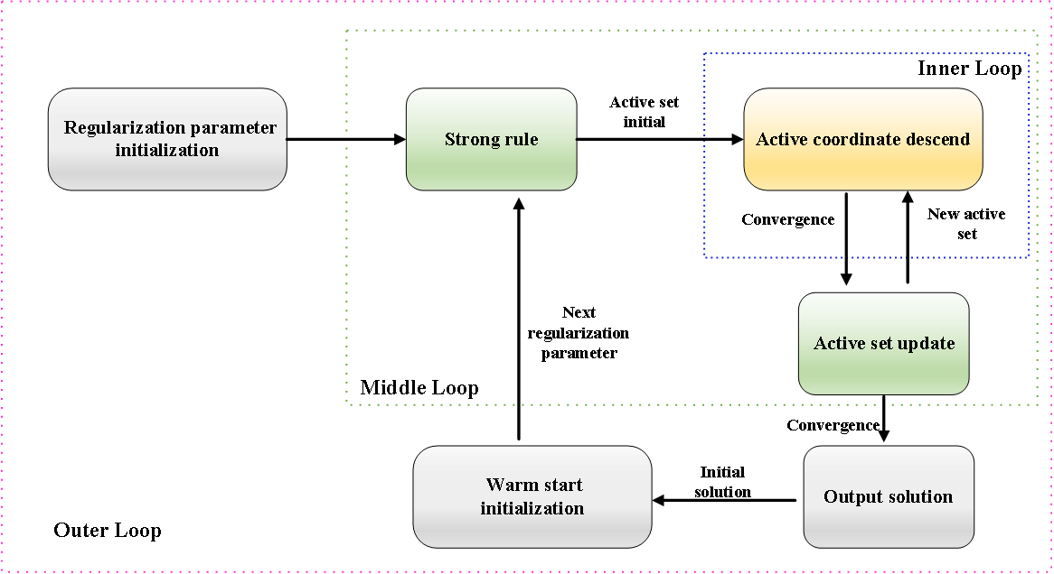
It is time-consumption to update all coordinates, a homotopy coordinate descent optimization framework is proposed to the computational time, which integrates the warm start initialization, active set updating strategy, and strong rule for coordinate pre-selection into the classical coordinate optimization. These three strategies constitute three nested loops for the proposed algorithm, as illustrated in Fig. 1. For simplicity, we first introduce its inner loop, then its middle loop, and at last its outer loop.

1. Inner Loop: Iterating over Coordinates within an Active Set. The inner loop is denoted as active coordinate descent (ActCooDes) algorithm. The iteration index for the inner loop is $(t)$, where $t=0,1,2,...$. The ActCooDes algorithm solves (3) by conducting exact coordinate minimization iteratively, but it only updates a subset of all coordinates, which is called ”active set”. Accordingly, the complementary set to the active set is called ”inactive set”, whose coordinates do not change throughout all iterations of the inner loop. Since the active set usually contains few number of coordinates, ActCooDes algorithm is very scalable and efficient.

We denote the active and inactive sets as $A$ and $\bar{A}$ respectively. According to the initial solution of the inner loop $\bm{\alpha}^{(0)}$, active set and inactive set are selected based on the sparse pattern:

Then ActCooDes algorithm minimizes (3) with all coordinates of $\bar{A}$ keeping at zero values, the objective function becomes:

Without loss of generality, we assume $\left|A\right|=s$, $A=\left\{j_{1}...,j_{s}\right\}\subseteq\left\{1,...,K\right\}$, where $j_{1}\leqslant j_{2}\leqslant...\leqslant j_{s}$. Given a solution $\bm{\alpha}^{(t)}$ at $t-th$ iteration, we construct a sequence of auxiliary solutions $\left\{\bm{w}^{\left(t+\text{1,}k\right)}\right\}_{k=0}^{s}$ to obtain $\bm{\alpha}^{(t+1)}$. Particularly, for $k=0$, we have $\bm{w}^{\left(t+\text{1,}0\right)}=\bm{\alpha}^{\left(t\right)}$; For $k=1,...,s$, we use (5) to update $w_{j_{k}}^{\left(t+\text{1,}k\right)}$ and make $\bm{w}_{\backslash j_{k}}^{\left(t+\text{1,}k\right)}=\bm{w}_{\backslash j_{k}}^{\left(t+\text{1,}k-1\right)}$.

Then we set $\bm{\alpha}^{\left(t+1\right)}=\bm{w}^{\left(t+\text{1,}s\right)}$ for the next iteration. The ActCooDes algorithm is terminated when

where $\tau$ is a small convergence parameter (i.e., $10^{-5}$).

The outline of inner loop is presented in Algorithm 1

2. Middle Loop: Updating Active Sets Iteratively. Since the inner loop can only converge to a local optimal solution of (7), it is not necessarily the local optimal solution of (3). Therefore, the inner loop needs to be combined with some active set updating scheme, which allows the active set to be changed. This leads to the middle loop of HCD.

The middle loop is denoted as iterative active set updating (IteActUpd) algorithm, and the iteration index for it is $[m]$, where $m=0,1,2,...$. As shown in Algorithm 2, the IteActUpd algorithm simultaneously updates the active set and decreases the objective value to ensure that the HCD algorithm converges to a local optimal solution of (3).

(1) Strong Rule for Active Set Initialization: Tibshirani et al. [39] suggest a aggressive active set initialization procedure for PICASSO using a ”strong rule”, which often leads to superior computational performance in practice. Inspired by this, we also propose a ”strong rule” for our HCD algorithm to initial active set. Suppose an initial solution $\bm{\alpha}^{[0]}$ is supplied to the middle loop, given an active set initialization parameter $\varphi\in\left(\text{0,}1\right)$, the strong rule for HCD initializes $A_{0}$ and $\bar{A}_{0}$ as:

where $\nabla_{j}f\left(\bm{\alpha}^{\left[0\right]}\right)$ denotes the $j-th$ entry of $\nabla f\left(\bm{\alpha}^{\left[0\right]}\right)$, and $\nabla f\left(\bm{\alpha}\right)$ is the gradient of $f(\bm{\alpha})=\frac{1}{2}||\bm{x}-\bm{D\alpha}||^{2}_{2}$. Note that the initialization parameters $\varphi$ need to be a reasonably small value (i.e., 0.1). Otherwise, the ”strong rule” will choose too many active coordinates and affect the sparsity of the solution.

(2) Active Set Updating Strategy: Suppose at the $m-th$ iteration $(m\geq 1)$, we obtain a solution $\bm{\alpha}^{[m]}$ with a pair of active and inactive sets defined as:

Each iteration of IteActUpd algorithm consists of two stages. The first stage is to conduct the ActCooDes algorithm over the active set $A_{m}$ until convergence, and then return a solution $\bm{\alpha}^{\left[m+0.5\right]}$. Since the coordinate descent algorithm may produce zero values for some active set coordinates, we remove these coordinates from the active set and update the active and inactive sets as follows:

The second stage checks which coordinates of $\bar{A}_{m+0.5}$ should be added into the active set. We propose a greedy selection rule for updating the active set. Particularly, let $\nabla_{j}f\left(\bm{\alpha}^{\left[m+0.5\right]}\right)$ denote the $j-th$ entry of $\nabla f\left(\bm{\alpha}^{\left[m+0.5\right]}\right)$, we select a coordinate by

The IteActUpd algorithm is terminated if

where $\delta$ is a small convergence parameter (e.g., $10^{-5}$). Otherwise, we take

and update the active and inactive set as:

The outline of middle loop is presented in Algorithm 2.

3. Outer Loop: Iterating over Regularization Parameter. The outer loop of HCD is the homotopy strategy which provides a warm starting initialization (WarStaInt). In the outer loop, we first set a large initial value of the regularization parameter $\lambda$ and gradually decrease it with a common ratio $\eta\in\left(\text{0,}1\right)$ until it reach to the target value $\lambda_{tgt}$. For every fixed value of the regularization parameter, the IteActUpd algorithm is used to search an approximate optimal solution of (3), which is set as the initial solution of the next iteration. Usually, the next loop with warm starting will require fewer iterations than current loop [28]. We set the initial regularization parameter as $\lambda_{0}=\lVert\bm{D}^{T}\bm{x}\rVert_{\infty}$ as with most algorithms. An outline of the WarStaInt algorithm is described as Algorithm 3.

For a fixed $\lambda_{n}$, suppose the middle loop iterates to the $m-th$ time and $|A_{m}|=s$. For $i\in A_{m}$, it has been proven that [37, 38]

while for $i\in\bar{A}_{m}$, $\varPhi_{\lambda_{n}}\left(\alpha_{i}^{(t+1)}\right)=\varPhi_{\lambda_{n}}\left(\alpha_{i}^{(t)}\right)$.

Thus, for all $\alpha_{i}^{(t+1)}\ (i=1,2,...,K)$, we have

It implies that

where $T_{m+0.5}$ is the number of iterations of ActCooDes in $m-th$ iteration of middle loop.

Similarly, we have

this inequality implies that, for a fixed $\lambda_{n}$, $\varPhi_{\lambda_{n}}\left\{\bm{\alpha}^{\left[m\right]}\right\}$ is nonincreasing. Since $f(\bm{\alpha})$ is bounded below, it then follows that ${\varPhi}_{\lambda_{n}}\left\{\bm{\alpha}^{\left[m\right]}\right\}$ is bounded below. Hence, ${\varPhi}_{\lambda_{n}}\left\{\bm{\alpha}^{\left[m\right]}\right\}$ converges to a finite value as $m\rightarrow\infty$ and a local optimal solution $\bm{\alpha}_{\lambda_{n}}^{*}$ can be achieved.

Since the $\lambda$ is monotone decreased, and $\bm{\alpha}_{\lambda_{n}}^{*}$ is set as the initial solution for IteActUpd in $\lambda_{n+1}$, we obtain that:

it implies that the objective value is monotone decreasing and a local optimal solution can be achieved by the proposed algorithm.

In the experiments, we use normal distribution and uniform distribution to generate simulate signals. For normal distribution, we firstly randomly generated the dictionary $\bm{D}\in R^{d\times K}$ with mean 0 and standard deviation 1, the vector $\bm{\alpha}^{*}\in R^{K}$ was generated with the same distribution at $s$ randomly chosen coordinates ($||\bm{\alpha}^{*}||_{0}=s$), the noise $\bm{z}\in R^{d}$ is a dense vector with independent random entries with mean 0 and standard deviation $\sigma$. For uniform distribution, the entries of $\bm{D}$ are generated independently with the uniform distribution over the interval $[-1,+1]$, the noise is a dense vector with independent random entries with the uniform distribution over the interval $[-\sigma,\sigma]$, where $\sigma$ is the noise magnitude. Finally, the observed signal $\bm{x}\in R^{d}$ is generated as $\bm{x}=\bm{D\alpha^{*}}+\bm{z}$.

For natural signals, we randomly extracted $10$ image patches from Barbara and Lena images to generate natural signals. Barbara image is noise-free and Lena image has random gaussian noise with $\sigma=10$. The patch size of Barbara and Lena are $8\times 8$ and $16\times 16$, respectively (it means the dimension $d$ of observed signal are 64 and 256, respectively). The dictionary is randomly generated with normal distribution and be normalized, the number of atoms are set as $K=256$ and $K=1024$, respectively. The average results of $10$ image patches are recorded for comparison.

In the experiments, unless otherwise stated, all parameters are set as follows. The initial value $\lambda_{0}$ of all algorithms is set as $\lVert\bm{D}^{T}\bm{x}\rVert_{\infty}$, the initial solution is set as $\bm{\alpha}^{0}=\bm{0}$. Other parameters are set as: $\tau=10^{-6}$, $\delta=10^{-3}$, $\varphi=0.05$, $\eta=0.5$.

In this part, we generated normal distributed noise-free signal with $(d=300,K=2000,s=20)$ to verify the proposed method, the regularization parameter $\lambda_{tgt}$ is set as $0.01$, 20 repeated trials are carried out and average results are recorded. Fig. 2 and Fig. 3 show two cases of the scatter diagram of reconstructed signal and convergence curve, and Tab. I presents the average results on the validation metrics. As it can be seen from Fig. 2 and Fig. 3 that the solution $\bm{\hat{\alpha}}$ obtained by our algorithm coincides completely with the original sparse signal $\bm{\alpha}^{*}$, which indicates that our algorithm can achieve the optimal solution and has strong reconstruction performance, the results presented in Tab. I also indicate the effectiveness of our algorithm. From Fig. 2 and Fig. 3 we can see that, only a dozen iterations can our algorithm convergent to the terminate condition, and from Tab. I we can see the average time spent of our algorithm to reconstruct the sparse signal is only $0.6074$ seconds. This two results indicate that the convergence speed of our algorithm is very fast which is applicable in practice.

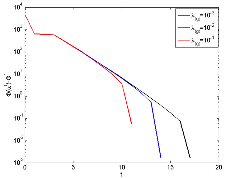
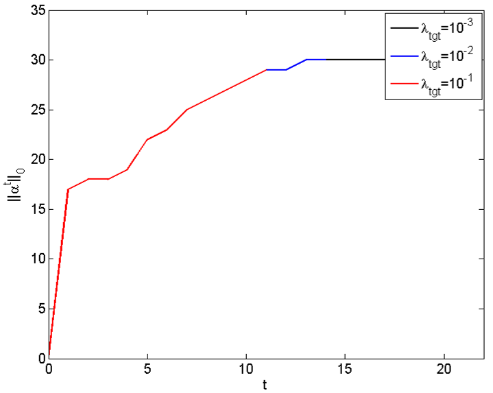
In this part, we investigate the sensitivity of parameters $\lambda_{tgt}$ and $\eta$ in HCD. First, the normal distributed noisy signal with $(d=400,K=2000,s=30,\sigma=0.01)$ is generated to evaluate the influence of regularization parameter $\lambda_{tgt}$, the results with different values of $\lambda_{tgt}$ are shown in Fig. 4. From this figure it can be seen that when $\lambda_{tgt}=10^{-3}$ or $10^{-2}$, HCD can obtain the same solution. While when $\lambda_{tgt}=10^{-1}$, the solution obtained is a litter more sparse than original sparse signal and results in a large objective gap, but is still acceptable. Therefore, within a certain range of $\lambda_{tgt}$, it only has a great influence on the number of iterations which will not influence the final result. In particular, it can be seen from Fig.4 that, despite $\lambda_{tgt}$ is changed, HCD traced the same solution path in previous iterations. The experimental results show that the proposed algorithm is robust to the regularization parameter, and it is unnecessary to spend too much time on parameter tuning.

In order to evaluate the influence of $\eta$ in HCD, we generated uniform distributed noisy signal with $(d=500,K=2000,s=50,\sigma=0.01)$ to do the experiment, the results with different values of $\eta$ are shown in Fig. 5. It can be seen from this figure that, though different values of $\eta$ can get similar results, the number of iterations of the algorithm gradually increases as $\eta$ increases. However, if $\eta$ is too small (i.e., 0.2), the gap between two adjacent values of $\lambda$ is too large, which will make HCD take more time to search for the solution (the CPU time of HCD with respect to these three values of $\eta$ are $2.44s$, $1.47s$ and $1.79s$, respectively). Therefore, for the following experiments, $\eta$ is set as $0.5$.

In this part, we show the superiority of our algorithm comparing with state-of-the-art SC algorithms. (1) Generated signal: we generated normal distributed noisy signal with $(d=256,K=1024,s=32,\sigma=0.01)$ and uniform distributed noisy signal with $(d=1000,K=5000,s=100,\sigma=0.01)$ for comparison. In the first case, the $\lambda_{tgt}$ of HCD, HIHT and AHIHT are set as $0.01$ while it is set as $0.1$ for PICASSO and PGH in order to get sparse solution. In the second case, $\lambda_{tgt}$ is set as $0.01$ for HCD, HIHT and AHIHT, and $0.5$ for PICASSO and PGH. The performance results of each algorithm are shown in Fig. 6 and Fig. 7, respectively.

Fig. 6 shows the objective gap versus the number of iterations $t$, from it we can see that HCD can obtain the lowest $ogj\_gap$ than the other four algorithms. From Fig. 6 it can be seen that PGH obtained a much larger reconstruction error than the other four algorithms, while the other four algorithms get similar results. It can be seen from Fig. 6 that, the sparsity of the sequences $\{\bm{\alpha}^{t}\}$ generated by PGH and HIHT algorithms oscillate much during the iteration process. However, the sparsity generated by HCD, AHIHT and PICASSO do not oscillate, and is almost increasing with the number of iterations, they are always searcher the solution in a sparse path. Fig. 6 shows the number of iterations of each $\lambda_{n}$. We can see that all stages of HCD and AHIHT took only 1 inner iterations and PICASSO took only 1 to 3 inner iterations to reach the relative precision, while PGH and HIHT took much inner iterations at each stage. We can make the conclusion that the two kinds of coordinate descent methods and AHIHT are more effective and efficient in reconstructing sparse representation than PGH and HIHT, while HCD and AHIHT are even better than PICASSO, this proves that $l_{0}$-norm is more effective than $l_{p}$-norm ($0<p\leq 1$) in reconstructing sparse representation. Fig. 7 demonstrates the same conclusion as Fig. 6

(2) Natural signal: In this experiment, $\lambda_{tgt}$ is set as $0.01$ for HCD and HIHT, while for PGH and PICASSO it is set as $0.1$, and it is tuned for AHIHT to get a reasonable result. Since $\bm{\alpha}^{*}$ is unknown, we compare these algorithms in terms of reconstruction error, sparsity and reconstruction time, the results are shown in Tab. II. It can be seen from this table that, AHIHT fails to produce sparse representation for nature signal when the atoms of dictionary are normalized ($||\bm{d}_{i}||_{2}=1,\forall i$), while this condition is always made in practical applications to avoid trivial solution. Compared with PGH, the other three algorithms can get a more sparse solution while maintain a lower reconstruction error, indicating that the other three algorithms can obtain a better local optimal solution. Compared with HIHT, PICASSO and HCD have improved the performance of sparse coding when applied in image reconstruction, while HCD is ever better than PICASSO. In term of reconstruction time, HIHT gets the lowest computational time (expect AHIHT) due to HIHT updates all coordinates in parallel, while the computational time of our algorithm is also acceptable. For high-dimensional data, HCD has achieved a significant reduction in computational time compared with PICASSO, indicating that HCD is more suitable than PICASSO for learning the sparse representation for high-dimensional signals and more applicable in practice. Therefore, compared with the other four algorithms, our algorithm achieves a better balance between reconstruction performance and computational time, and can learn the sparse representation for natural signal more effectively.

References

- [1] C. L. P. Chen, L. Liu, L. Chen, Y. Y. Tang, and Y. Zhou, “Weighted couple sparse representation with classified regularization for impulse noise removal,” IEEE Transactions on Image Processing, vol. 24, no. 11, pp. 4014–4026, 2015.
- [2] L. Liu, C. L. P. Chen, X. You, Y. Y. Tang, Y. Zhang, and S. Li, “Mixed noise removal via robust constrained sparse representation,” IEEE Transactions on Circuits and Systems for Video Technology, vol. 28, no. 9, pp. 2177–2189, 2018.
- [3] R. Tibshirani, “Regression shrinkage and selection via the lasso,” Journal of the Royal Statal Society: Series B (Methodological), vol. 58, no. 1, 1996.
- [4] T. Pang, F. Nie, J. Han, and X. Li, “Efficient feature selection via -norm constrained sparse regression,” IEEE Transactions on Knowledge and Data Engineering, vol. 31, no. 5, pp. 880–893, 2019.
- [5] Z. Jiang, Z. Lin, and L. S. Davis, “Label consistent k-svd: Learning a discriminative dictionary for recognition,” IEEE Transactions on Pattern Analysis and Machine Intelligence, vol. 35, no. 11, pp. 2651–2664, 2013.
- [6] N. Akhtar and A. Mian, “Nonparametric coupled bayesian dictionary and classifier learning for hyperspectral classification,” IEEE Transactions on Neural Networks and Learning Systems, vol. 29, no. 9, pp. 4038–4050, 2018.
- [7] S. Mallat and Z. Zhang, “Matching pursuits with time-frequency dictionaries.” IEEE Transactions on Signal Processing, vol. 41, no. 12, pp. 3397–3415, 1993.
- [8] S. Chen, D. Donoho, and M. Saunders, “Atomic decomposition by basis pursuit,” SIAM Review, vol. 43, no. 1, pp. 129–159, 2001.
- [9] R. Chartrand, “Exact reconstruction of sparse signals via nonconvex minimization,” IEEE Signal Processing Letters, vol. 14, no. 10, pp. 707–710, 2007.
- [10] Z. Xu, X. Chang, F. Xu, and H. Zhang, “ regularization: A thresholding representation theory and a fast solver,” IEEE Transactions on Neural Networks and Learning Systems, vol. 23, no. 7, pp. 1013–1027, 2012.
- [11] X. Chen, M. K. Ng, and C. Zhang, “Non-lipschitz -regularization and box constrained model for image restoration,” IEEE Transactions on Image Processing, vol. 21, no. 12, pp. 4709–4721, 2012.
- [12] L. Qin, Z. C. Lin, Y. She, and Z. Chao, “A comparison of typical minimization algorithms,” Neurocomputing, vol. 119, no. 16, pp. 413–424, 2013.
- [13] Y. C. Pati, R. Rezaiifar, and P. Krishnaprasad, “Orthogonal matching pursuit: recursive function approximation with applications to wavelet decomposition.” in IEEE International Conference on Signal, Systems and Computers, vol. 1, 1993, pp. 40–44.
- [14] D. L. Donoho, Y. Tsaig, I. Drori, and J. L. Starck, “Sparse solution of underdetermined systems of linear equations by stagewise orthogonal matching pursuit,” IEEE Transation on Information Theory, vol. 58, no. 2, pp. 1094–1121, 2012.
- [15] M. K. Tan, I. W. Tsang, and L. Wang, “Matching pursuit lasso part i: Sparse recovery over big dictionary,” IEEE Transation on Signal Processing, vol. 68, no. 3, pp. 723–741, 2015.
- [16] ——, “Matching pursuit lasso part ii: Applications and sparse recovery over batch signals,” IEEE Transatioon on Signal Processing, vol. 68, no. 3, pp. 742–753, 2015.
- [17] C. A. Loza, “Robomp: Robust variants of orthogonal matching pursuit for sparse representations,” PeerJ Computer Science, vol. 5, p. e192, 2019.
- [18] D. Donoho and M. Elad, “Optimally sparse representation in general (nonorthogonal) dictionaries via minimization.” in Proceeding of the National Academy of Sciences of the United States of America, vol. 100, no. 5, 2003, pp. 2197–2202.
- [19] E. J. Candes and T. Tao, “Near-optimal signal recovery from random projections: Universal encoding strategies?” IEEE Transactions on Information Theory, vol. 52, no. 12, pp. 5406–5425, 2006.
- [20] A. Y. Yang, A. Ganesh, Z. H. Zhou, S. S. Sastry, and Y. Ma, “A review of fast -minimization algorithm for robust face recognition,” Proceedings of the International Conference on Computer Vision and Pattern Recognition, pp. 1–36, 2010.
- [21] M. A. T. Figueiredo, R. D. Nowak, and S. J. Wright, “Gradient projection for sparse reconstruction: Application to compressed sensing and other inverse problems,” IEEE Journal of Selected Topics in Signal Processing, vol. 1, no. 4, pp. 586–597, 2007.
- [22] S. J. Kim, K. Koh, and S. Boyd, “An interior-point method for large-scale -regularized least squares,” IEEE Journal on Selected Topics in Signal Processing, vol. 1, no. 4, pp. 606–617, 2007.
- [23] M. C. D. Malioutov and A. Willsky, “Homotopy continuation for sparse signal representation,” Proceedings of the IEEE International Conference on Acoustics, Speech, and Signal Processing, 2005.
- [24] B. P. M. Osborne and B. Turlach, “A new approach to variable selsection in least squares problems,” IMA Journal of Numercial Analysis, vol. 20, pp. 389–404, 2000.
- [25] P. Combettes and V. Wajs, “Signal recovery by proximal forward-backward splitting,” SIAM Multiscale Modeling and Simulation, vol. 4, pp. 1168–1200, 2005.
- [26] M. D. I. Daubechies and C. Mol, “An iterative thresholding algorithm for linear inverse problems with a sparsity constraint,” Communications on Pure and Applied Math, vol. 57, pp. 1413–1457, 2004.
- [27] E. T. Hale, W. Yin, and Y. Zhang, “A fixed-point continuation method for -regularized minimization with applications to compressed sensing,” CAAM Tech Report TR07-07, pp. 1–45, 2007.
- [28] R. N. S. J. Wright and M. Figueiredo, “Sparse reconstruction by separable approximation,” IEEE Transactions on Signal Processing, vol. 57, no. 7, pp. 2479–2493, 2009.
- [29] A. Beck and M. Teboulle, “A fast iterative shrinkage-thresholding algorithm for linear inverse problems,” SIAM Journal on Imaging Sciences, vol. 2, no. 1, pp. 183–202, 2009.
- [30] X. Lin and Z. Tong, “A proximal-gradient homotopy method for the sparse least-squares problem,” SIAM Journal on Optimization, vol. 23, no. 2, pp. 1062–1091, 2013.
- [31] J. Yang and Y. Zhang, “Alternating direction algorithms for -problems incompressive sensing,” (preprint) arXiv:0912.1185, 2009.
- [32] X. G. Li, J. Ge, H. M. Jiang, M. D. Wang, M. Y. Hong, and T. Zhao, “Boosting pathwise coordinate optimization in high dimensions: Sequential screening and proximal sub-sampled newton algorithm,” Technical report, Georgia Tech, 2017.
- [33] T. Zhao, H. Liu, and T. Zhang, “Pathwise coordinate optimization for nonconvex sparse learning: Algorithm and theory,” Annals of Statistics, 2017.
- [34] J. Ge, X. G. Li, H. M. Jiang, H. Liu, T. Zhang, M. Y. Hong, and T. Zhao, “Picasso: A sparse learning library for high dimensional data analysis in r and python,” Journal of Machine Learning Research, vol. 20, pp. 1–5, 2019.
- [35] T. Blumensath and M. E. Davie, “Iterative thresholding for sparse approximations,” Fourier Analysis and Applications, vol. 27, no. 5, pp. 629–654, 2008.
- [36] ——, “Iterative hard thresholding for compressed sensing,” Applied and Computational Harmonic Analysis, vol. 27, no. 3, pp. 265–274, 2009.
- [37] Z. S. Lu, “Iterative hard thresholding methods for regularized convex cone programming,” Mathematical Programming, vol. 147, pp. 125–154, 2012.
- [38] Z. Dong and W. Zhu, “Homotopy methods based on -norm for compressed sensing,” IEEE Transactions on Neural Networks and Learning Systems, vol. 29, no. 4, pp. 1132–1146, 2018.
- [39] R. Tibshirani, J. Bien, J. Friedman, T. Hastie, N. Simon, J. Taylor, and R. J. Tibshirani, “Strong rules for discarding predictors in lasso-type problems,” Journal of the Royal Statal Society. Series B, Statal methodology, vol. 74, no. 2, pp. 245–266, 2012.