Clustering microbiome data using mixtures of logistic normal multinomial models

Suppose we have $K+1$ bacterial taxa for a sample denoted as a random vector $\mathbf{W}=(W_{1},\dots,W_{K+1})^{\top}$. Here, the taxa could represent any level of the bacterial phylogeny such as OTU, species, genus, phylum, etc. Due to the fact that taxa counts from 16S sequencing can only reveal relative abundance, let’s suppose there is a vector $\mbox{\boldmath{$\Theta$}}=(\Theta_{,}\dots,\Theta_{K+1})$ such that $\sum_{k=1}^{K+1}{\Theta_{k}}=1$, which represents the underlying composition of the bacterial taxa. Then, the microbial taxa count $\mathbf{W}$ can be modeled as a multinomial random variable with the following conditional density function:

$$p(\mathbf{w}|\mbox{\boldmath{$\Theta$}})\propto\prod_{k=1}^{K+1}(\Theta_{k})^{w_{k}}.$$

Several models have been proposed in the literature that capture the relative abundance nature of microbiome data and analyze the compositional data Holmes et al. 2012; Xia et al. 2013. Here we use the model by Xia et al Xia et al. 2013 that utilizes an additive log-ratio transformation $\phi(\mbox{\boldmath{$\Theta$}})$ proposed by Aitchison Aitchison 1982 such that:

$$\mathbf{Y}=\phi(\mbox{\boldmath{$\Theta$}})=\left(\log\left(\dfrac{\Theta_{1}}{\Theta_{K+1}}\right),\dots,\log\left(\dfrac{\Theta_{K}}{\Theta_{K+1}}\right)\right)^{\top}.$$

(1)

This transformation $\phi$ maps the vector $\Theta$ from a $K$-dimensional simplex to the $K$-dimensional real space $\mathbb{R}^{K}$ while $\mathbf{Y}$ is assumed to follow a multivariate normal distribution with mean $\mu$ and covariance $\Sigma$ with the density function

$$p(\mathbf{y}|\mbox{\boldmath{$\mu$}},\mbox{\boldmath{$\Sigma$}})\propto|\mbox{\boldmath{$\Sigma$}}|^{-\frac{1}{2}}\exp\left\{-\frac{1}{2}(\mathbf{y}-\mbox{\boldmath{$\mu$}})^{\top}\mbox{\boldmath{$\Sigma$}}^{-1}(\mathbf{y}-\mbox{\boldmath{$\mu$}})\right\}.$$

As this additive log-ratio transformation is a one-to-one map, the inverse operator of $\phi$ exists and is given by

$$\mbox{\boldmath{$\Theta$}}=\phi^{-1}(\mathbf{Y})=\begin{cases}\dfrac{\exp(Y_{k})}{1+\sum_{k=1}^{K}{\exp(Y_{k})}}&k=1,\dots,K\\ \dfrac{1}{1+\sum_{k=1}^{K}{\exp(Y_{k})}}&k=K+1\end{cases}.$$

Hence, the joint density of $\mathbf{W}$ and $\mathbf{Y}$ up to a constant is as follows:

$$\begin{split}p(\mathbf{w},\mathbf{y})&\propto p\left(\mathbf{w}|\phi^{-1}(\mathbf{y})\right)p(\mathbf{y}|\mbox{\boldmath{$\mu$}},\mbox{\boldmath{$\Sigma$}})=\prod_{k=1}^{K+1}\left({\phi^{-1}(\mathbf{y})}_{k}\right)^{w_{k}}\times|\mbox{\boldmath{$\Sigma$}}|^{-\frac{1}{2}}\exp\left\{-\frac{1}{2}(\mathbf{y}-\mbox{\boldmath{$\mu$}})^{\top}\mbox{\boldmath{$\Sigma$}}^{-1}(\mathbf{y}-\mbox{\boldmath{$\mu$}})\right\}\end{split}.$$

For the microbiome data, only the count vector $\mathbf{W}$ are observed while the latent variable $\mathbf{Y}$ is unobserved. The marginal density of $\mathbf{W}$ can be written as

$$p(\mathbf{w})=\int_{\mathbb{R}^{K}}p(\mathbf{w},\mathbf{y})d\mathbf{y}\propto\int_{\mathbb{R}^{K}}\prod_{k=1}^{K+1}\left({\phi^{-1}(\mathbf{y})}_{k}\right)^{w_{k}}\times|\mbox{\boldmath{$\Sigma$}}|^{-\frac{1}{2}}\exp\left\{-\frac{1}{2}(\mathbf{y}-\mbox{\boldmath{$\mu$}})^{\top}\mbox{\boldmath{$\Sigma$}}^{-1}(\mathbf{y}-\mbox{\boldmath{$\mu$}})\right\}d\mathbf{y}.$$

Note that this marginal distribution of $\mathbf{W}$ involves multiple integrals and cannot be further simplified. Here, in presence of missing data, an expectation-maximization algorithm Dempster et al. 1977 or some variant of it is typically utilized for parameter estimation. An EM-algorithm comprises two steps: an E-step in which the expected value of the complete data (i.e. observed and missing data) log-likelihood is computed given the observed data and current parameter estimate and an M-step in which the complete data log-likelihood is maximized. These step are repeated until convergence to obtain the maximum likelihood estimate of the parameters. To compute the expected value of the complete data log-likelihood, $\mathbb{E}(\mathbf{Y}\mid\mathbf{w})$ and $\mathbb{E}(\mathbf{Y}\mathbf{Y}^{T}\mid\mathbf{w})$ needs to be computed for which we need $p(\mathbf{y}|\mathbf{w})$. Mathematically,

$\displaystyle p(\mathbf{y}|\mathbf{w})=\frac{p(\mathbf{w},\mathbf{y})}{p(\mathbf{w})}=\frac{\prod_{k=1}^{K+1}\left({\phi^{-1}(\mathbf{y})}_{k}\right)^{w_{k}}\times|\mbox{\boldmath{$\Sigma$}}|^{-\frac{1}{2}}\exp\left\{-\frac{1}{2}(\mathbf{y}-\mbox{\boldmath{$\mu$}})^{\top}\mbox{\boldmath{$\Sigma$}}^{-1}(\mathbf{y}-\mbox{\boldmath{$\mu$}})\right\}}{\int_{\mathbb{R}^{K}}\prod_{k=1}^{K+1}\left({\phi^{-1}(\mathbf{y})}_{k}\right)^{w_{k}}\times|\mbox{\boldmath{$\Sigma$}}|^{-\frac{1}{2}}\exp\left\{-\frac{1}{2}(\mathbf{y}-\mbox{\boldmath{$\mu$}})^{\top}\mbox{\boldmath{$\Sigma$}}^{-1}(\mathbf{y}-\mbox{\boldmath{$\mu$}})\right\}d\mathbf{y}}.$

However, the denominator involves multiple integrals and cannot be further simplified. One could employ a Markov chain Monte Carlo (MCMC) approach to explore the posterior state space; however, these methods are typically computational expensive, especially for high-dimensional problems. Here, we propose the use of variational Gaussian approximation (VGA) Barber and Bishop 1998 for parameter estimation. A VGA aims to find an optimal and tractable approximation that has a Gaussian parametric form to approximate the true complex posterior by minimizing the Kullback-Leibler divergence between the true and the approximating densities. It has been successfully used in many practical applications to overcome this challenge.Bishop 2006; Archambeau et al. 2007; Wainwright et al. 2008; Khan et al. 2012; Challis and Barber 2013; Arridge et al. 2018. In order to utilize VGA, we define a new latent variable $\eta$ by transforming $\mathbf{Y}$ such that

$$\mbox{\boldmath{$\eta$}}=B\mathbf{Y},\quad\text{ where }B=\begin{pmatrix}1&0&\dots&0\\ 0&1&\dots&0\\ \vdots&\vdots&\dots&\vdots\\ 0&0&\dots&1\\ 0&0&\dots&0\end{pmatrix},$$

(2)

is a $(K+1)\times K$ matrix which takes the form as an identity matrix attached by a row of K zeros. Given that $\mathbf{Y}\sim\mathop{\rm N}(\mbox{\boldmath{$\mu$}},\mbox{\boldmath{$\Sigma$}})$, the new latent variable $\mbox{\boldmath{$\eta$}}\sim\mathop{\rm N}(\tilde{\mbox{\boldmath{$\mu$}}},\tilde{\mbox{\boldmath{$\Sigma$}}})$ where

$$\tilde{\mbox{\boldmath{$\mu$}}}=B\mbox{\boldmath{$\mu$}}=(\mbox{\boldmath{$\mu$}},0)^{\top};\quad\tilde{\mbox{\boldmath{$\Sigma$}}}=B\mbox{\boldmath{$\Sigma$}}B^{\top}=\begin{pmatrix}\mbox{\boldmath{$\Sigma$}}&\vline&\mathbf{0}_{K\times 1}\\ \hline\cr\mathbf{0}_{1\times K}&\vline&0\end{pmatrix}.$$

(3)

Then, the underlying composition variable $\Theta$ can be written as a function of $\eta$:

$$\mbox{\boldmath{$\Theta$}}=\tilde{\phi}^{-1}(\mbox{\boldmath{$\eta$}})=\dfrac{\exp{\eta_{k}}}{\sum_{k=1}^{K+1}{\exp{\eta_{k}}}}k=1\dots,K+1.$$

(4)

Suppose we have an approximating density $q(\mbox{\boldmath{$\eta$}})$, then the marginal log density of $\mathbf{W}$ can be written as:

	$\displaystyle\log p(\mathbf{w})$	$\displaystyle=\int\log p(\mathbf{w})~q(\mbox{\boldmath{$\eta$}})~d\mbox{\boldmath{$\eta$}}$
		$\displaystyle=\int\log\frac{p(\mathbf{w},\mbox{\boldmath{$\eta$}})/q(\mbox{\boldmath{$\eta$}})}{p(\mbox{\boldmath{$\eta$}}\mid\mathbf{w})/q(\mbox{\boldmath{$\eta$}})}~q(\mbox{\boldmath{$\eta$}})~d\mbox{\boldmath{$\eta$}}$
		$\displaystyle=\int\left[\log~p(\mathbf{w},\mbox{\boldmath{$\eta$}})-\log q(\mbox{\boldmath{$\eta$}})\right]~q(\mbox{\boldmath{$\eta$}})~d\mbox{\boldmath{$\eta$}}+\int\log\dfrac{q(\mbox{\boldmath{$\eta$}})}{p(\mbox{\boldmath{$\eta$}}|\mathbf{w})}~q(\mbox{\boldmath{$\eta$}})~d\mbox{\boldmath{$\eta$}}$
		$\displaystyle=F(q(\mbox{\boldmath{$\eta$}}),\mathbf{w})+D_{KL}(q||p),$

where the first part $F(q(\mbox{\boldmath{$\eta$}}),\mathbf{w})=\int q(\mbox{\boldmath{$\eta$}})\log\dfrac{p(\mathbf{w},\mbox{\boldmath{$\eta$}})}{q(\mbox{\boldmath{$\eta$}})}d\mbox{\boldmath{$\eta$}}$ is called the evidence lower bound (ELBO) Barber and Bishop 1998 and the second part $D_{KL}(q||p)=\int\log\dfrac{q(\mbox{\boldmath{$\eta$}})}{p(\mbox{\boldmath{$\eta$}}|\mathbf{w})}~q(\mbox{\boldmath{$\eta$}})~d\mbox{\boldmath{$\eta$}}$ is the Kullback-Leibler divergence from $p(\mbox{\boldmath{$\eta$}}|\mathbf{w})$ to $q(\mbox{\boldmath{$\eta$}})$. Hence, minimizing the Kullback-Leibler divergence is equivalent to maximizing the following evidence lower bound (ELBO). In VGA, we assume $q(\mbox{\boldmath{$\eta$}})$ is a Gaussian distribution, such that

$$q(\mbox{\boldmath{$\eta$}})=\mathop{\rm N}(\mbox{\boldmath{$\eta$}}|\mathbf{m},V)\propto|V|^{-\frac{1}{2}}\exp\left\{-\frac{1}{2}(\mbox{\boldmath{$\eta$}}-\mathbf{m})^{\top}V^{-1}(\mbox{\boldmath{$\eta$}}-\mathbf{m})\right\}.$$

Given the fact that $q(\mbox{\boldmath{$\eta$}})$ is fully characterized by its mean vector and covariance matrix, the above lower bound is a function of the variational parameters $\mathbf{m}$ and $V$ and we aim to find the optimal set of $(\mathbf{m},V)$ such that it maximizes $F(q(\mbox{\boldmath{$\eta$}},\mathbf{w}))$. $F(q(\mbox{\boldmath{$\eta$}},\mathbf{w}))$ can be separated into three parts:

$$F(q(\mbox{\boldmath{$\eta$}}),\mathbf{w})=F(\mathbf{m},V)=-\int q(\mbox{\boldmath{$\eta$}})\log q(\mbox{\boldmath{$\eta$}})d\mbox{\boldmath{$\eta$}}+\int q(\mbox{\boldmath{$\eta$}})\log p(\mbox{\boldmath{$\eta$}})d\mbox{\boldmath{$\eta$}}+\int q(\mbox{\boldmath{$\eta$}})\log p(\mathbf{w}|\mbox{\boldmath{$\eta$}})d\mbox{\boldmath{$\eta$}}.$$

Up to a constant, the last integral, which is denoted as $\gamma$, in the above decomposition is given as follows:

$$\begin{split}\gamma&=\int q(\mbox{\boldmath{$\eta$}})\log p(\mathbf{w}|\mbox{\boldmath{$\eta$}})d\mbox{\boldmath{$\eta$}}\\ &=\mathbb{E}_{q(\mbox{\boldmath{$\eta$}}|\mathbf{m},V)}\left[\mathbf{w}^{\top}\mbox{\boldmath{$\eta$}}-\sum_{k=1}^{K+1}{w_{k}\log\left(\sum_{k=1}^{K+1}{\exp\eta_{k}}\right)}\right]\\ &=\mathbf{w}^{\top}\mathbf{m}-\left(\sum_{k=1}^{K+1}w_{k}\right)\mathbb{E}_{q(\mbox{\boldmath{$\eta$}}|\mathbf{m},V)}\left[\log\left(\sum_{k=1}^{K+1}{\exp\eta_{k}}\right)\right].\end{split}$$

Similar to Blei and Lafferty,Blei and Lafferty 2006 we use an upper bound for the expectation of log sum exponential term with a Taylor expansion,

$$\mathbb{E}_{q(\mbox{\boldmath{$\eta$}}|\mathbf{m},V)}\left[\log\left(\sum_{k=1}^{K+1}{\exp\eta_{k}}\right)\right]\leq\xi^{-1}\left\{\sum_{k=1}^{K+1}\mathbb{E}_{q(\mbox{\boldmath{$\eta$}}|\mathbf{m},V)}\left[\exp(\eta_{k})\right]\right\}-1+\log(\xi),$$

where $\xi\in\mathbb{R}$ is introduced as a new variational parameter.

Here, we further assume that $V$ is a diagonal matrix with the first $K$ diagonal element of $V$ as $v_{k}^{2}$ and the $K+1^{th}$ diagonal element is set to 0 such that

$$v_{k}^{2}=\begin{cases}v_{k}^{2},&k=1,\dots,K\\ 0,&k=K+1.\end{cases}$$

We also denote the $k-$th element of $\mathbf{m}$ as $m_{k}$ such that

$$m_{k}=\begin{cases}m_{k},&k=1,\dots,K\\ 0,&k=K+1.\end{cases}$$

Hence, the expectation

$$\mathbb{E}_{q(\mbox{\boldmath{$\eta$}}|\mathbf{m},V)}\left[\exp(\eta_{k})\right]=\exp\left(m_{k}+\dfrac{v_{k}^{2}}{2}\right),\text{ for }k=1,\dots,K+1.$$

Based on this upper bound, we obtain a concave lower bound to $\gamma$ and to the ELBO. The new concave variational Gaussian lower bound to the model evidence $\log p(\mathbf{w})$ is given as follows

$$\begin{split}\tilde{F}\left(\mathbf{m},V,\tilde{\mbox{\boldmath{$\mu$}}},\tilde{\mbox{\boldmath{$\Sigma$}}},\xi\right)&=\mathbf{w}^{\top}\mathbf{m}-\left(\sum_{k=1}^{K+1}w_{k}\right)\left\{\xi^{-1}\left[\sum_{k=1}^{K+1}\exp\left(m_{k}+\dfrac{v_{k}^{2}}{2}\right)\right]-1+\log(\xi)\right\}\\ &-\frac{1}{2}\log|B^{\top}\tilde{\mbox{\boldmath{$\Sigma$}}}B|-\frac{1}{2}(\mathbf{m}-\tilde{\mbox{\boldmath{$\mu$}}})^{\top}\tilde{\mbox{\boldmath{$\Sigma$}}}^{\ast}(\mathbf{m}-\tilde{\mbox{\boldmath{$\mu$}}})-\frac{1}{2}\mathop{\rm Tr}(\tilde{\mbox{\boldmath{$\Sigma$}}}^{\ast}V)\\ &+\frac{1}{2}\sum_{k=1}^{K}\log(v_{k}^{2})+\dfrac{K}{2},\end{split}$$

(5)

where

$$\tilde{\mbox{\boldmath{$\Sigma$}}}^{\ast}=\begin{pmatrix}\mbox{\boldmath{$\Sigma$}}^{-1}&\vline&\mathbf{0}_{K\times 1}\\ \hline\cr\mathbf{0}_{1\times K}&\vline&0\end{pmatrix},$$

is the generalized inverse of $\tilde{\mbox{\boldmath{$\Sigma$}}}$. Details on the derivation of this lower bound can be found in Appendix A. Given fixed $\mathbf{w}$, $\tilde{\mbox{\boldmath{$\mu$}}}$, and $\tilde{\mbox{\boldmath{$\Sigma$}}}$, this lower bound only depends on the variational parameter set $(\mathbf{m},V,\xi)$.

Maximization of the lower bound $\tilde{F}\left(\mathbf{m},V,\tilde{\mbox{\boldmath{$\mu$}}},\tilde{\mbox{\boldmath{$\Sigma$}}},\xi\right)$ with respect to $\xi$ has a closed form solution and is given by

$$\hat{\xi}=\sum_{k=1}^{K+1}\exp\left(m_{k}+\dfrac{v_{k}^{2}}{2}\right).$$

(6)

However, maximization with respect to $\mathbf{m}$ and $v_{k},k=1,\dots,K$ do not possess analytical solutions. We use Newton’s method to search for roots to the following derivatives:

$$\dfrac{\partial\tilde{F}}{\partial\mathbf{m}}=\mathbf{w}-\tilde{\mbox{\boldmath{$\Sigma$}}}^{\ast}(\mathbf{m}-\tilde{\mbox{\boldmath{$\mu$}}})-\left(\sum_{k=1}^{K+1}w_{k}\right)\xi^{-1}\exp\left(\mathbf{m}+\dfrac{\mathbf{v}^{2}}{2}\right),$$

(7)

with $\mathbf{v}^{2}=(v_{1}^{2},\dots,v_{K}^{2},0)$ denoting the diagonal element of $V$ as a vector; and

$$\dfrac{\partial\tilde{F}}{\partial v_{k}}=v_{k}^{-1}-v_{k}\tilde{\mbox{\boldmath{$\Sigma$}}}_{k,k}^{\ast}-\left(\sum_{k=1}^{K+1}w_{k}\right)\xi^{-1}\exp\left(m_{k}+\dfrac{v_{k}^{2}}{2}\right)v_{k}.$$

(8)

Details can be found in Appendix A.

Assume there are $G$ subgroups in the population, with $\pi_{g}$ denoting the mixing weight of the $g-$th component such that $\sum_{g=1}^{G}\pi_{g}=1$. Then, a $G-$component finite mixtures logistic normal multinomial models can be written as

$$f(\mathbf{w}\mid\bm{\vartheta})=\sum_{g=1}^{G}\pi_{g}f_{g}(\mathbf{w}\mid\vartheta_{g}),$$

where $f_{g}(\mathbf{w}\mid\bm{\vartheta}_{g})$ represents the density function of the observation $\mathbf{W}=\mathbf{w}$, given that $\mathbf{W}$ comes from the $g-$th component with parameters $\vartheta_{g}$.

Provided $n$ observed counts, $\mathbf{w}=(\mathbf{w}_{1},\dots,\mathbf{w}_{n})$ with a transformed underlying the composition $\mathbf{Y}_{i},i=1,\dots,n$, the likelihood of a $G-$component finite mixture is given as

$$\mathcal{L}(\bm{\vartheta}\mid\mathbf{w})=\prod_{i=1}^{n}f(\mathbf{w}_{i}\mid\bm{\vartheta})=\prod_{i=1}^{n}\sum_{g=1}^{G}\pi_{g}f_{g}(\mathbf{w}_{i}\mid\vartheta_{g})=\prod_{i=1}^{n}\sum_{g=1}^{G}\pi_{g}\int p(\mathbf{w}_{i}\mid\mathbf{y}_{i})p(\mathbf{y}_{i}\mid\vartheta_{g})d\mathbf{y}_{i}.$$

In clustering, the unobserved component membership is denoted by an indicator variable $z_{ig},i=1,\dots,n,g=1,\dots,G$ that takes the form

$$z_{ig}=\begin{cases}1&\text{ if the }i-th\text{ observation is from the }g-th\text{ group},\\ 0&\text{ otherwise}.\end{cases}$$

Therefore, conditional on $z_{ig}$, we have

$$\mathbf{Y}_{i}|z_{ig}=1\sim\mathop{\rm N}(\mbox{\boldmath{$\mu$}}_{g},\mbox{\boldmath{$\Sigma$}}_{g}).$$

In order to utilize the variational approach for parameter estimation, we again define a new latent variable $\eta$ such that $\mbox{\boldmath{$\eta$}}=B\mathbf{Y}$ and

$$\mbox{\boldmath{$\eta$}}_{i}\mid z_{ig}=1\sim\mathop{\rm N}(\tilde{\mbox{\boldmath{$\mu$}}}_{g},\tilde{\mbox{\boldmath{$\Sigma$}}}_{g}),~\text{where}~\tilde{\mbox{\boldmath{$\mu$}}}_{g}=B\mbox{\boldmath{$\mu$}}_{g}=(\mbox{\boldmath{$\mu$}}_{g},0)^{\top}~\text{and}~\tilde{\mbox{\boldmath{$\Sigma$}}}_{g}=B\mbox{\boldmath{$\Sigma$}}_{g}B^{\top}=\begin{pmatrix}\mbox{\boldmath{$\Sigma$}}_{g}&\vline&\mathbf{0}_{K\times 1}\\ \hline\cr\mathbf{0}_{1\times K}&\vline&0\end{pmatrix}.$$

Therefore, the complete data (i.e., observed counts $\mathbf{W}$ and unobserved class label indicator variable) log-likelihood using the marginal density of $\mathbf{W}$ is

$\displaystyle\ell$

$\displaystyle=\log\left[\prod_{i=1}^{n}\prod_{g=1}^{G}\pi_{g}f_{g}(\mathbf{w}_{i}\mid\vartheta_{g})\right]^{z_{ig}}=\sum_{i=1}^{n}\sum_{g=1}^{G}z_{ig}\left\{\log\pi_{g}+\log\left[\int p(\mathbf{w}_{i}|\mbox{\boldmath{$\eta$}}_{i})p(\mbox{\boldmath{$\eta$}}_{i}|\tilde{\mbox{\boldmath{$\mu$}}}_{g},\tilde{\mbox{\boldmath{$\Sigma$}}}_{g})d\mbox{\boldmath{$\eta$}}_{i}\right]\right\}.$

To perform variational inference on the mixture model, we substitute $\log\left[\int p(\mathbf{w}_{i}|\mbox{\boldmath{$\eta$}}_{i})p(\mbox{\boldmath{$\eta$}}_{i}|\mbox{\boldmath{$\mu$}}_{g},\mbox{\boldmath{$\Sigma$}}_{g})d\mbox{\boldmath{$\eta$}}_{i}\right]$ by the variational Gaussian lower bound $\tilde{F}\left(\mathbf{m},V,\tilde{\mbox{\boldmath{$\mu$}}},\tilde{\mbox{\boldmath{$\Sigma$}}},\xi\right)$ derived in Section 2.2. Hence, the variational Gaussian lower bound of complete data log likelihood can be written as:

$$\begin{split}\tilde{\mathcal{L}}=&\sum_{i=1}^{n}\sum_{g=1}^{G}z_{ig}\log\pi_{g}+\sum_{i=1}^{n}\sum_{g=1}^{G}z_{ig}\mathbf{w}_{i}^{\top}\mathbf{m}_{ig}\\ &-\sum_{i=1}^{n}\sum_{g=1}^{G}z_{ig}\left(\sum_{k=1}^{K+1}w_{ik}\right)\left\{\xi_{i}^{-1}\left[\sum_{k=1}^{K+1}\exp\left(m_{igk}+\dfrac{v_{igk}^{2}}{2}\right)\right]-1+\log(\xi_{i})\right\}\\ &+\sum_{i=1}^{n}\sum_{g=1}^{G}z_{ig}\left\{\frac{1}{2}\log|B^{\top}\tilde{\mbox{\boldmath{$\Sigma$}}}_{g}B|-\frac{1}{2}(\mathbf{m}_{ig}-\tilde{\mbox{\boldmath{$\mu$}}}_{g})^{\top}\tilde{\mbox{\boldmath{$\Sigma$}}}_{g}^{\ast}(\mathbf{m}_{ig}-\tilde{\mbox{\boldmath{$\mu$}}}_{g})\right.\\ &\quad\quad\quad\quad\quad\quad\quad\left.-\frac{1}{2}\mathop{\rm Tr}(\tilde{\mbox{\boldmath{$\Sigma$}}}_{g}^{\ast}V_{ig})+\frac{1}{2}\sum_{k=1}^{K}\log(v_{igk}^{2})+\dfrac{K}{2}\right\}.\end{split}$$

(9)

Hence, we need to find optimal solutions to variational parameters $(\mathbf{m}_{ig},V_{ig},\xi_{i})$ that are associated with each observation $\mathbf{w}_{i},i=1,\dots,n$, as well as the model group-specific Gaussian parameters $(\tilde{\mbox{\boldmath{$\mu$}}}_{g},\tilde{\mbox{\boldmath{$\Sigma$}}}_{g}),g=1,\ldots,G$, such that the complete data variational Gaussian lower bound $\tilde{\mathcal{L}}$ is maximized. The use of VGA provides great reduction in the computational time.

Parameter estimation can be done in an iterative EM-type approach, from here on referred to as variational EM such that the following steps are iterated until convergence. For the parameters that do not have a closed form solution to the optimization, we perform one step of Newton’s method to approximate the root to their first derivatives.

1. Step 1:

   Conditional on the variational parameters $(\mathbf{m}_{ig},V_{ig},\xi_{i})$ and model group-specific Gaussian parameters $(\tilde{\mbox{\boldmath{$\mu$}}}_{g},\tilde{\mbox{\boldmath{$\Sigma$}}}_{g})$, $\mathbb{E}(Z_{ig}\mathbf{W}_{i})$ is computed. Given $(\tilde{\mbox{\boldmath{$\mu$}}}_{g},\tilde{\mbox{\boldmath{$\Sigma$}}}_{g})$,

   $$\mathbb{E}\left(Z_{ig}\mid\mathbf{w}_{i}\right)=\frac{\pi_{g}f_{g}(\mathbf{w}_{i}\mid\tilde{\mbox{\boldmath{$\mu$}}}_{g},\tilde{\mbox{\boldmath{$\Sigma$}}}_{g})}{\sum_{h=1}^{G}\pi_{h}f_{h}(\mathbf{w}_{i}\mid\tilde{\mbox{\boldmath{$\mu$}}}_{h},\tilde{\mbox{\boldmath{$\Sigma$}}}_{h})}.$$

   This involves the marginal distribution of $\mathbf{W}$ and hence, we use an approximation of $\mathbb{E}\left(Z_{ig}\mid\mathbf{w}_{i}\right)$ where we replace the marginal density $\mathbf{W}$ by the exponent of ELBO such that

   $$\hat{z}_{ig}:=\dfrac{\pi_{g}\exp\left\{\tilde{F}\left(\mathbf{w}_{i},\mathbf{m}_{ig},V_{ig},\tilde{\mbox{\boldmath{$\mu$}}}_{g},\tilde{\mbox{\boldmath{$\Sigma$}}}_{g},\xi_{i}\right)\right\}}{\sum_{j=1}^{G}\pi_{j}\exp\left\{\tilde{F}\left(\mathbf{w}_{i},\mathbf{m}_{ij},V_{ij},\tilde{\mbox{\boldmath{$\mu$}}}_{j},\tilde{\mbox{\boldmath{$\Sigma$}}}_{j},\xi_{i}\right)\right\}}.$$

2. Step 2:

   Update $\hat{\xi}_{i},\hat{\mathbf{m}}_{ig},\hat{V}_{ig}$:

   • •

     update $\hat{\xi}_{i}$ according to Equation 6;

   • •

     update $\hat{\mathbf{m}}_{ig}$ by performing one step of Newton’s method for approximating the root to the derivative in Equation 7, then let $\hat{m}_{ig(K+1)}=0$;

   • •

     for $k=1,\dots,K$, update $\hat{v}_{igk}^{2}$ by performing one step of Newton’s method searching root to the derivative in Equation  8, let $\hat{v}_{ig(K+1)}^{2}=0$, then $\hat{V}_{ig}=\mathop{\rm diag}(\hat{v}_{ig1}^{2},\dots,\hat{v}_{ig(K+1)}^{2})$.

3. Step 3:

   Update $\pi_{ig}$, $\tilde{\mbox{\boldmath{$\mu$}}}_{g}$ and $\tilde{\mbox{\boldmath{$\Sigma$}}}_{g}$ as

   	$\displaystyle\hat{\pi}_{ig}$	$\displaystyle=\frac{\sum_{n=1}^{n}\hat{z}_{ig}}{n},$
   	$\displaystyle\hat{\tilde{\mbox{\boldmath{$\mu$}}}}_{g}$	$\displaystyle=\dfrac{\sum_{i=1}^{n}\hat{z}_{ig}\hat{\mathbf{m}}_{ig}}{\sum_{i=1}^{n}\hat{z}_{ig}},$
   	$\displaystyle\hat{\tilde{\mbox{\boldmath{$\Sigma$}}}}_{g}$	$\displaystyle=\dfrac{\sum_{i=1}^{n}\hat{z}_{ig}\left[\hat{V}_{ig}+(\hat{\mathbf{m}}_{ig}-\hat{\tilde{\mbox{\boldmath{$\mu$}}}}_{g})(\hat{\mathbf{m}}_{ig}-\hat{\tilde{\mbox{\boldmath{$\mu$}}}}_{g})^{\top}\right]}{\sum_{i=1}^{n}\hat{z}_{ig}}.$

Note that the original parameters $\mbox{\boldmath{$\mu$}}_{g}$ and $\mbox{\boldmath{$\Sigma$}}_{g}$ can be obtained by the transformation

$$\hat{\mbox{\boldmath{$\mu$}}}_{g}=B^{\top}\hat{\tilde{\mbox{\boldmath{$\mu$}}}}_{g};\quad\hat{\mbox{\boldmath{$\Sigma$}}}_{g}=B^{\top}\hat{\tilde{\mbox{\boldmath{$\Sigma$}}}}_{g}B.$$

An Aitken acceleration criterionAitken 1926 is employed to stop the iterations. More specifically, at $t^{th}$ iteration, when $t>2$, calculate

$$\begin{split}a^{(t-1)}&=\dfrac{\ell^{(t)}-\ell^{(m-1)}}{\ell^{(t-1)}-\ell^{(t-2)}},\\ \ell_{\infty}^{(t)}&=\ell^{(t-1)}+\dfrac{1}{1-a^{(t-1)}}\left(\ell^{(t)}-\ell^{(t-2)}\right),\end{split}$$

where $\ell^{(t)}=\tilde{F}\left(\mathbf{w}_{i},\mathbf{m}_{ig},V_{ig},\tilde{\mbox{\boldmath{$\mu$}}}_{g},\tilde{\mbox{\boldmath{$\Sigma$}}}_{g},\xi_{i}\right)$ is the variational Gaussian lower bound who approximates the log likelihood at $t^{th}$ iteration. Then, the algorithm will be stopped when $\left|\ell_{\infty}^{(t)}-\ell_{\infty}^{(t-1)}\right|<\epsilon$ for a given $\epsilon$Böhning et al. 1994. In our analysis, we $\epsilon$ is set to be $1\times 10^{-3}$.

In the clustering context, the number of components $G$ is unknown. Hence, one typically fits models for a large range of possible $G$ and the number of clusters is then chosen a posteriori using a model selection criteria. The Bayesian information criterion (BIC)Schwarz 1978 is one of the most popular criteria in the model-based clustering literature.McNicholas 2016

$$\text{BIC}\approx-2\tilde{\mathcal{L}}+d\log(n),$$

where $\tilde{\mathcal{L}}$, defined in Equation 9, is the variational Gaussian lower bound of the complete data log likelihood, and $d$ is the number of free parameters in the model. Specifically, when fitting a $G-$ component model, $d=\frac{(K+1)K}{2}\times G+K\times G+G-1$.

When the true class labels are known (e.g., in simulation studies), we assess the performance of our proposed model using the adjusted Rand index (ARI)Hubert and Arabie 1985. It is a measure of the pairwise agreement between the predicted and true classifications such that an ARI of 1 indicates perfect classification and $0$ indicates that the classification obtained is no better than by chance.

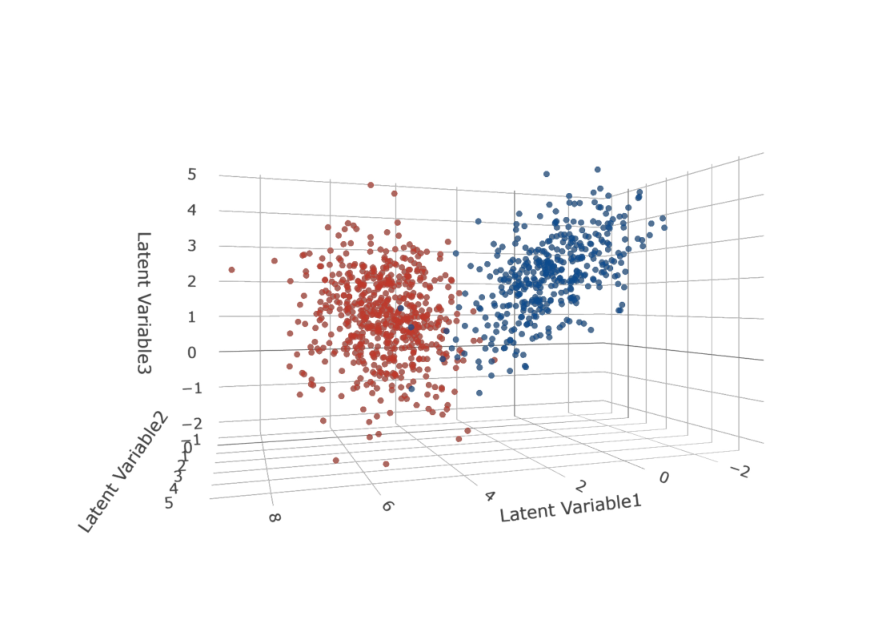
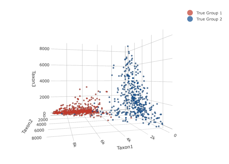
In this simulation study, we generated $100$ datasets where the underlying latent variable $\mathbf{Y}$ came from two component, three-dimensional multivariate Gaussian distributions with mixing proportions $\mbox{\boldmath{$\pi$}}=(0.6,0.4)$; see Figure 1 (left panel). The first component consists of $n_{1}=600$ observations and the second component consists of $n_{2}=400$ observations. The parameters used to generate the datasets are summarized in Table 1. We fitted the models with $G=1,\ldots,5$ on all $100$ datasets. In $100$ out of $100$ datasets, BIC selected a two-component model. The models selected by BIC yielded an average ARI $=0.94$ with standard deviation $0.02$. The average and standard deviation of the estimated parameters for the all $100$ datasets using the VGA approach are summarized in Table 1 and using the hybrid approach are summarized in Table 2. Note that the parameter estimation using both approaches are very close to the true value of the parameters. Average computation time for Simulation Study 1 using the proposed VGA approach was 200.97 (sd of 35.39) minutes on a single-core processor. It took additional on average 45.14 (sd of 15.84) minutes for one iteration of the full Bayesian. Thus, the mean computation time using the hybrid approach was 246.11 (sd of 38.57) minutes. Figure 2 illustrates a clear difference in the distribution of the relative abundance of taxa in the two predicted groups. We also ran the Dirichlet-multinomial mixture model for $G=1:4$ and selected the best model using BIC. In all 100 out of 100 datasets, it selected a $G=4$ model with an average ARI of 0.52 (sd of 0.04). The Dirichlet-multinomial model overestimates the number of components by splitting the true clusters into multiple clusters with some misclassifications among them.

In this simulation study, we generated $100$ datasets with the underlying latent variable $\mathbf{Y}$ from three component five-dimensional multivariate Gaussian distributions (see Figure 3 for the pairwise scatterplot of the underlying latent variable $\mathbf{Y}_{i}$).

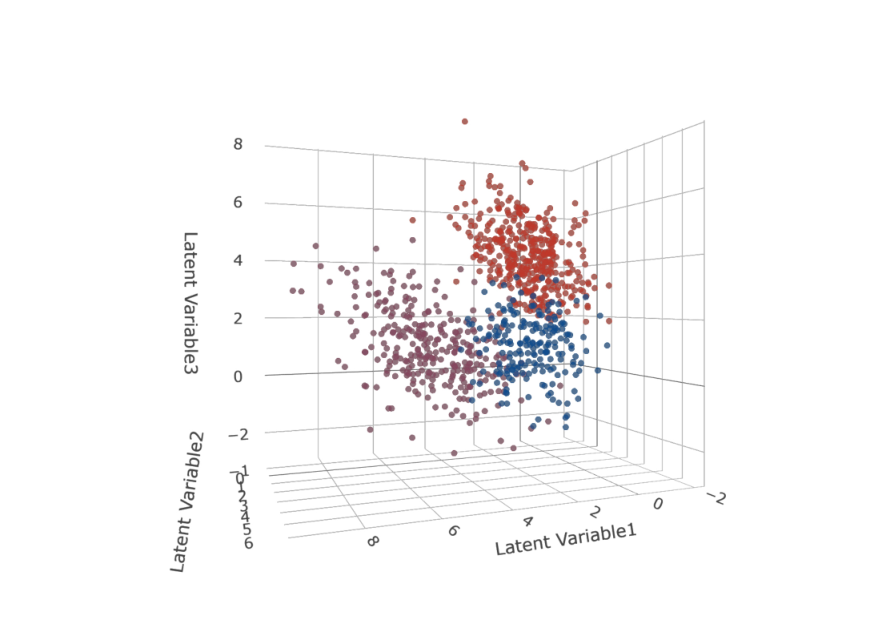
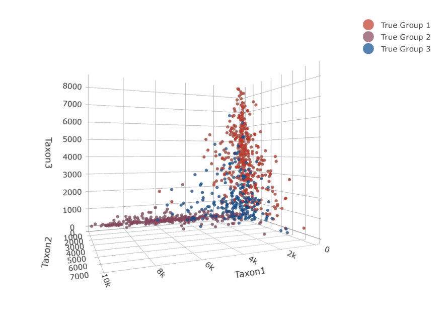
There are $n_{1}=300$ observations in Group 1, $n_{2}=400$ observations in Group 1, and $n_{3}=200$ observations in Group 3. The true parameters are summarized in Table 3. Figure 4 (left panel) shows the first three dimensions of the latent variable $\mathbf{Y}_{i}$’s and Figure 4 (right panel) shows the first three dimensions of the observed counts $\mathbf{W}_{i}$’s. There is a more separation between the groups when visualizing the latent variables as opposed to the observed counts.

The proposed algorithm was applied on all $100$ datasets where for each dataset, we fitted the models with for $G=1,\dots,4$. In 94 out of the 100 datasets, a $G=3$ model was selected using the BIC, a $G=2$ was selected for 3 out of the 100 datasets, and $G=4$ models were selected for the remaining 3 datasets. The overall mean ARI for all 100 datasets was 0.93 (sd of 0.06) and the mean ARI for 94 datasets where a three component model was selected was 0.94 (sd of 0.01). The average and standard deviation of the estimated parameters for the all $100$ datasets using the VGA approach are summarized in Table 3 and using the hybrid approach are summarized in Table 4. Note that the parameter estimation using both approaches are very close to the true value of the parameters. Average computation time for Simulation Study 1 using the proposed VGA approach was 214.91 (sd of 35.91) minutes on a single-core processor. It took additional on average 40.84 (sd of 16.64) minutes for one iteration of the full Bayesian. Thus, the mean computation time for the hybrid approach was 255.74 (sd of 42.70) minutes. Figure 5 illustrates a clear difference in the distribution of the relative abundance of taxa in the predicted groups. We also ran the Dirichlet-multinomial mixture model for $G=1:4$ and selected the best model using BIC. In all 100 out of 100 datasets, it selected a $G=4$ model with an average ARI of 0.33 (sd of 0.03).

To test the performance of the proposed algorithm on higher dimensional datasets, as well as datasets generated from mixture of Dirichlet-multinomial models, we performed a series of 10 additional simulation studies, each containing 100 datasets, as described below:

• •

  Generate 100 datasets from a two-component mixture of logistic normal multinomial models with each of the following:

  • –

    $K$, the dimension of the latent variable, being $5,10,$ and $20$;

  • –

    $n$, the sample size, being $100,200,$ and $500$.

  • –

    True parameters are the same for different $n$ but same $K$.

• •

  Generate 100 datasets from mixture of two-component Dirichlet-multinomial models with dimension 6, and sample size of 200.

We ran the proposed algorithm for $G=1:5$ on all datasets and used BIC for model selection. We also applied the Dirichlet-multinomial mixture (DMM) models on these datasets with BIC for model selection. Table 5 shows the number of times the correct model ($G=2$) was selected out of 100 datasets for each simulation study, as well as the average ARI with standard deviation, for the proposed algorithm and the Dirichlet-multinomial mixture models.

When data were generated from a mixture of logistic normal multinomial models, in all simulation scenarios, the proposed algorithm identified the correct number of components for more than 80 times out of 100 with average ARI $\geq 0.96$, except for the case with $K=20,n=100$. Note that in the later case, the number of parameters needed to be estimated is far larger than the sample size. Also, it is observed that, in general, when sample size increases, performance of the proposed algorithm in terms of the number of times it selects the correct model as well as the average ARI also increases. However, the Dirichlet-multinomial mixture model did not perform as well on data simulated from the logistic normal multinomial mixture models. Even in the case of $K=20,n=200$, where it correctly selected the two-component model 99 out of 100 times, the average ARI was only 0.6286 with standard deviation of 0.1284.

When the data was generated from the Dirichlet-multinomial mixture models, our proposed model is able to recover the underlying cluster in 85 out of the 100 datasets with an average ARI of $0.8957$ and standard deviation of $0.0916$ whereas the Dirichlet-multinomial mixture model was able to recover the underlying cluster structure in all 100 datasets with an average ARI of 0.9589 (sd=0.0456). When performing each simulation study, the computational job was distributed onto a computer cluster, where the proposed algorithm applied on each one of the 100 datasets was run on a one-core slot. Table 5 summarizes the average elapsed time for running the proposed algorithm in minutes, with standard deviation. For most cases, it takes the proposed algorithm less than 60 minutes. As the number of observations and the dimensionality of data increases, the time to convergence increased as well.

Table 6 summarizes how many times each $G=1:5$ were selected by the proposed algorithm. In nine out of the ten studies, our approach was able to identify the correct number of components in at least 85 out of 100 datasets. For the scenario when $K=20$ and $n=100$ (small sample size and high dimensional), both proposed algorithm and the Dirichlet-multinomial mixture model approach favoured a one-component model. We also summarized the average of $L_{1}$ norm between the true parameters and the estimated values along with the standard errors for the simulations with data generated from mixture of logistic normal multinomial models in Table 7. It shows that, when the dimensionality is low, the proposed algorithm can not only identify the correct underlying group structure but also is able to recover the true parameters well. As the dimensionality increases, the proposed algorithm can still capture the true number of components in the data with high classification accuracy and the estimated central location parameter ($\mu$) is also estimated close to the true value. However, the estimation of the spread parameter ($\Sigma$) become less precise as dimensionality becomes higher; however, the distance between the true and the estimated parameters decreases as the sample size becomes larger.

We applied our proposed algorithms to four microbiome datasets from three studies:

• •

  The Ferretti 2018 Dataset: We applied our algorithm to the Ferretti 2018 dataset (Ferretti et al. 2018) available through the R package curatedMetagenomicData (Pasolli et al. 2017) as FerrettiP_2018 dataset. The study aims to understand the acquisition and development of the infant microbiome and assessed the impact of the maternal microbiomes on the development of infant oral and fecal microbial communities from birth to 4 months of life. Twenty five mother infant pairs who vaginally delivered healthy newborns at full term were recruited for the study. For each mother, stool (proxy for gut microbiome), dorsum tongue swabs (for oral microbiome), vaginal introitus swabs (for vaginal microbiome), intermammary cleft swabs (skin microbiome) and breast milk were obtained. As the DNA extraction from breast milk was not feasible in most cases, they were not analyzed further. All infants were exclusively breastfed at 3 days, 96% at 1 month, and 56% at 4 months and for each newborn, oral cavity and gut samples were taken from birth to up to 4 months. The samples were sequenced using high-resolution shotgun metagenomics (Quince et al. 2017) with an improved strain-level computational profiling of known and poorly characterized microbiome members (Segata 2018). See Ferretti et al (2018) Ferretti et al. 2018 for further details. Here, we applied our algorithms to two subsets of the datasets: comparing gut microbiome of the infant with their mothers and comparing oral microbiome of the infants with their mothers.

  Gut microbiome subset: This subset of Ferretti 2018 dataset available through R package curatedMetagenomicData comprised of 119 samples (23 adults and 96 newborns). As mentioned in Ferretti et al (2018), stool samples of newborns were taken at five different time points: Day 1, Day 3, Day 7, 1 Month and 4 Months. As repeated measurements at different time points are taken on the same individuals and our model currently cannot model that (violates the independence assumption), we only focus on one time point (i.e., Day 1) for the newborns. Hence, the resulting dataset comprises of 42 individuals (23 adults and 19 infants). Here, we focused our analysis on the OTU counts at the genus level data.

  Oral microbiome subset: This subset of Ferretti 2018 dataset available through R package curatedMetagenomicData comprised of 62 samples (23 adults and 39 infants). As mentioned in Ferreti et al (2018), oral samples of infants were taken at two different time points: Day 1 and Day 3. Here, as the Day 3 had measurements for all 23 newborns, we use the Day 3 measurements for the analysis. The resulting dataset consists of 46 individuals (23 adults and 23 infants). Here, we again focused our analysis on the OTU counts at the genus level data.

• •

  The Shi 2015 Data: We also applied our algorithm to the Shi 2015 dataset (Shi et al. 2015) available through the R package curatedMetagenomicData (Pasolli et al. 2017) as Shi_2015 dataset. Periodontitis is a common oral disease that affects about 50% of the American adults and is associated with alterations in the subgingival microbiome of individual tooth sites. The study aimed to identify and predict the disease progression using the compositions of the subgingival microbiome. Samples were collected from 12 healthy individuals with chronic periodontitis from multiples tooth sites per individual, before and after nonsurgical therapy that consisted of scaling and root planing. Only the samples from the tooth sites that were clinically resolved after the therapy were selected for the study resulting in an average of two sites per subject. Although samples were obtained from multiple sites of individuals, Shi and colleagues (Shi et al. 2015) state that individual tooth sites are likely to have independent clinical states and unique microbial communities in subgingival pockets, and therefore, we treated them as independent samples for our analysis. This resulted in a total of 48 samples (24 periodontitis samples and 24 recovered samples).

• •

  The atlas1006 Data: We also applied our algorithm to the atlas1006 dataset available through the R package microbiome (Lahti et al. 2014). The dataset comprises of microbiome compositions of 1045 western adults with no reported health complications. Covariates information such as age, BMI category, sex, and nationality are also available. The BMI category was underweight ($n=21$), lean ($n$=484), overweight ($n=197$), obese ($n=222$), severe obese ($n=99$) and morbid-obese ($n=22$). For our analysis, we combined both underweight and lean into one category “lean” and obese, severe obese, and morbid-obese into one category “obese”, thus resulting in three BMI categories.

As our approach is currently not designed for high dimensional data, we first utilized the R package ALDEx2 (Fernandes et al. 2013; Gloor 2015) for differential abundance analysis on the observed genus counts to identify the genera that are different among different groups in the datasets. This step is analogous to conducting differential expression analysis in RNA-seq studies before performing cluster analysis to identify variables that are group differentiating. As the sample size of Ferretti 2018 and Shi 2015 datasets were less than 50, we only focused on a small set (top four) of differentially abundant genera and aggregated the remaining genera in a category “Others” to preserve relative abundance. For the atlas1006 dataset which has a sample size of $n=1045$, we used top 20 differentially abundant genera that were differentially abundant in “obese” and “lean” category. This “Other” genus was then used as the reference level for computing the underlying composition and conducting the additive log-ratio transformation. We applied our algorithm to this dataset for $G=1$ to $4$ on all datasets and used BIC for model selection. We also ran the Dirichlet-multinomial mixture model with the same set of genera for $G=1$ to $4$ on all datasets and utilized BIC for model selection. Summary of the clustering performances are provided in Table 8. In two out of the four datasets (i.e., the Ferretti gut microbiome dataset and the Shi dataset) our approach outperforms the Dirichlet-multinomial mixture models while both approaches provides a perfect classification on the Ferretti oral microbiome dataset. It is important to note that for the atlas1006 datasets, both approaches fail to recover the underlying group structure.

To visualize the true and recovered cluster structure, we conducted principal component analysis using the transformed variable $\mathbf{Y}$.

Two observations were misclassified in the Ferretti gut dataset using our proposed algorithm, and as can be seen in Figure 6, the misclassified infant had a similar microbiome composition to the adult and the misclassified adult had a similar microbiome composition to the infant. Similarly, as seen in Figure 6, most of the misclassified observations for the Shi dataset also had a similar microbiome composition to the group they were assigned. Shi and colleagues (Shi et al. 2015) also utilized the microbiome profiles to classify the clinical state. They performed a supervised classification using the weighted gene-voting algorithm and leave-one-out cross-validation yielding 33 out of 48 samples as correctly classified into the respective clinical state (correct classification rate of 68.75%) whereas 6 samples were misclassified into the incorrect clinical state and 9 samples were not assigned to any clinical state due to low prediction strength. Note that in supervised classification, the group labels are used to build a predictive model which is then used to make predictions on new or “future” observations. Here, we achieved a correction classification rate of 85.42% (i.e., 41/48 correct classification). On the atlas1006 dataset, recall that both the proposed algorithm and the Dirichlet-multinomial approach did not perform well in recovering the underlying groups based on the BMI. Visualization of the dataset using the principal components show that there is in fact not a clear separation in the microbiome compositions between the various BMI categories in the dataset. Although the recovered cluster structure does not correspond to the known BMI categories, Figure 6 shows that the proposed approach is able to recover homogenous clusters. We do not have further information to investigate what the recovered cluster structure can yield insight into

Based on suggestion from a reviewer, an alternate approach to using the differentially abundant taxa by using the most abundant taxa instead was investigated. To keep the dimensionality the same, for Ferretti and Shi datasets, we used the top 4 most abundant taxa and for the atlas1006 dataset, we used the top 20 most abundant taxa. We ran our proposed approach for $G=1,\ldots,4$ and used BIC for model selection. Our approach selected a one-component model (ARI of 0) for Ferretti gut microbiome dataset, a two-component model (ARI of 0.36, 9/46 misclassification) for Ferretti oral microbiome dataset, a two-component model (ARI of 0.05,18/48 misclassification) for the Shi dataset, and a two-component model (ARI of 0.002) for atlas1006 dataset. Note that using the most abundant genera for all four dataset resulted in a far lower ARI compared to using the most differentially abundant genera.

References

- (1)
- Äijö et al. (2018) Äijö, T., Müller, C. L. and Bonneau, R. (2018), ‘Temporal probabilistic modeling of bacterial compositions derived from 16s rrna sequencing’, Bioinformatics 34(3), 372–380.
- Aitchison (1982) Aitchison, J. (1982), ‘The statistical analysis of compositional data’, Journal of the Royal Statistical Society: Series B (Methodological) 44(2), 139–160.
- Aitken (1926) Aitken, A. C. (1926), ‘A series formula for the roots of algebraic and transcendental equations’, Proceedings of the Royal Society of Edinburgh 45, 14–22.
- Archambeau et al. (2007) Archambeau, C., Cornford, D., Opper, M. and Shawe-Taylor, J. (2007), ‘Gaussian process approximations of stochastic differential equations’, Journal of Machine Learning Research 1, 1–16.
- Arridge et al. (2018) Arridge, S. R., Ito, K., Jin, B. and Zhang, C. (2018), ‘Variational gaussian approximation for poisson data’, Inverse Problems 34(2), 025005.
- Barber and Bishop (1998) Barber, D. and Bishop, C. M. (1998), ‘Ensemble learning in bayesian neural networks’, Nato ASI Series F Computer and Systems Sciences 168, 215–238.
- Bishop (2006) Bishop, C. M. (2006), Pattern recognition and machine learning, springer.
- Blei and Lafferty (2006) Blei, D. and Lafferty, J. (2006), ‘Correlated topic models’, Advances in Neural Information Processing Systems 18, 147.
- Blei et al. (2017) Blei, D. M., Kucukelbir, A. and McAuliffe, J. D. (2017), ‘Variational inference: A review for statisticians’, Journal of the American Statistical Association 112(518), 859–877.
- Böhning et al. (1994) Böhning, D., Dietz, E., Schaub, R., Schlattmann, P. and Lindsay, B. G. (1994), ‘The distribution of the likelihood ratio for mixtures of densities from the one-parameter exponential family’, Annals of the Institute of Statistical Mathematics 46(2), 373–388.
- Bouveyron and Brunet-Saumard (2014) Bouveyron, C. and Brunet-Saumard, C. (2014), ‘Model-based clustering of high-dimensional data: A review’, Computational Statistics & Data Analysis 71, 52–78.
- Cao et al. (2017) Cao, Y., Zhang, A. and Li, H. (2017), ‘Multi-sample estimation of bacterial composition matrix in metagenomics data’, arXiv preprint arXiv:1706.02380 .
- Caporaso et al. (2011) Caporaso, J. G., Lauber, C. L., Costello, E. K., Berg-Lyons, D., Gonzalez, A., Stombaugh, J., Knights, D., Gajer, P., Ravel, J., Fierer, N. et al. (2011), ‘Moving pictures of the human microbiome’, Genome Biology 12(5), R50.
- Challis and Barber (2013) Challis, E. and Barber, D. (2013), ‘Gaussian kullback-leibler approximate inference’, The Journal of Machine Learning Research 14(1), 2239–2286.
- Chen and Li (2013) Chen, J. and Li, H. (2013), ‘Variable selection for sparse dirichlet-multinomial regression with an application to microbiome data analysis’, The Annals of Applied Statistics 7(1).
- Dempster et al. (1977) Dempster, A. P., Laird, N. M. and Rubin, D. B. (1977), ‘Maximum likelihood from incomplete data via the em algorithm’, Journal of the Royal Statistical Society: Series B (Methodological) 39(1), 1–22.
- Eckburg et al. (2005) Eckburg, P. B., Bik, E. M., Bernstein, C. N., Purdom, E., Dethlefsen, L., Sargent, M., Gill, S. R., Nelson, K. E. and Relman, D. A. (2005), ‘Diversity of the human intestinal microbial flora’, science 308(5728), 1635–1638.
- Fernandes et al. (2013) Fernandes, A., Macklaim, J., Linn, T., Reid, G. and Gloor, G. (2013), ‘Anova-like differential gene expression analysis of single-organism and meta-rna-seq’, PLoS One 8(7), e67019.
- Ferretti et al. (2018) Ferretti, P., Pasolli, E., Tett, A., Asnicar, F., Gorfer, V., Fedi, S., Armanini, F., Truong, D. T., Manara, S., Zolfo, M. et al. (2018), ‘Mother-to-infant microbial transmission from different body sites shapes the developing infant gut microbiome’, Cell Host & Microbe 24(1), 133–145.
- Fraher et al. (2012) Fraher, M. H., O’toole, P. W. and Quigley, E. M. (2012), ‘Techniques used to characterize the gut microbiota: a guide for the clinician’, Nature Reviews Gastroenterology & hepatology 9(6), 312.
- Frühwirth-Schnatter (2006) Frühwirth-Schnatter, S. (2006), Finite mixture and Markov switching models, Springer Science & Business Media.
- Ghahramani and Beal (1999) Ghahramani, Z. and Beal, M. (1999), ‘Variational inference for bayesian mixtures of factor analysers’, Advances in neural information processing systems 12.
- Gloor (2015) Gloor, G. (2015), ‘Aldex2: Anova-like differential expression tool for compositional data’, ALDEX manual modular 20, 1–11.
- Greenblum et al. (2012) Greenblum, S., Turnbaugh, P. J. and Borenstein, E. (2012), ‘Metagenomic systems biology of the human gut microbiome reveals topological shifts associated with obesity and inflammatory bowel disease’, Proceedings of the National Academy of Sciences 109(2), 594–599.
- Hamady and Knight (2009) Hamady, M. and Knight, R. (2009), ‘Microbial community profiling for human microbiome projects: Tools, techniques, and challenges’, Genome Research 19(7), 1141–1152.
- Haq et al. (2019) Haq, A. U., Zhang, D., Peng, H. and Rahman, S. U. (2019), ‘Combining multiple feature-ranking techniques and clustering of variables for feature selection’, IEEE Access 7, 151482–151492.
- Hartigan and Wong (1979) Hartigan, J. A. and Wong, M. A. (1979), ‘A k-means clustering algorithm’, Applied Statistics 28(1), 100–108.
- Holmes et al. (2012) Holmes, I., Harris, K. and Quince, C. (2012), ‘Dirichlet multinomial mixtures: generative models for microbial metagenomics’, PLOS One 7(2).
- Hubert and Arabie (1985) Hubert, L. and Arabie, P. (1985), ‘Comparing partitions’, Journal of classification 2(1), 193–218.
- Joseph et al. (2013) Joseph, N., Paulson, C., Corrada Bravo, H. and Pop, M. (2013), ‘Robust methods for differential abundance analysis in marker gene surveys’, Nature Methods 10, 1200–1202.
- Khan et al. (2012) Khan, E., Mohamed, S. and Murphy, K. P. (2012), Fast bayesian inference for non-conjugate gaussian process regression, in ‘Advances in Neural Information Processing Systems’, pp. 3140–3148.
- Koeth et al. (2013) Koeth, R. A., Wang, Z., Levison, B. S., Buffa, J. A., Org, E., Sheehy, B. T., Britt, E. B., Fu, X., Wu, Y., Li, L. et al. (2013), ‘Intestinal microbiota metabolism of l-carnitine, a nutrient in red meat, promotes atherosclerosis’, Nature Medicine 19(5), 576.
- Kuczynski et al. (2012) Kuczynski, J., Lauber, C. L., Walters, W. A., Parfrey, L. W., Clemente, J. C., Gevers, D. and Knight, R. (2012), ‘Experimental and analytical tools for studying the human microbiome’, Nature Reviews Genetics 13(1), 47–58.
- Lahti et al. (2014) Lahti, L., Salojärvi, J., Salonen, A., Scheffer, M. and De Vos, W. M. (2014), ‘Tipping elements in the human intestinal ecosystem’, Nature Communications 5(1), 1–10.
- Ley et al. (2006) Ley, R. E., Peterson, D. A. and Gordon, J. I. (2006), ‘Ecological and evolutionary forces shaping microbial diversity in the human intestine’, Cell 124(4), 837–848.
- Li (2015) Li, H. (2015), ‘Microbiome, metagenomics, and high-dimensional compositional data analysis’, Annual Review of Statistics and Its Application 2, 73–94.
- MacQueen (1967) MacQueen, J. B. (1967), Some methods for classification and analysis of multivariate observations. In Proceedings of the Fifth Berkeley Symposium on Mathematical Statistics and Probability, University of California Press, Berkeley, CA.
- McLachlan and Peel (2000) McLachlan, G. and Peel, D. (2000), Wiley series in probability and statistics, John Wiley & Sons Hoboken, NJ.
- McNicholas (2016) McNicholas, P. D. (2016), Mixture model-based classification, Chapman and Hall/CRC.
- Mcnicholas and Murphy (2008) Mcnicholas, P. D. and Murphy, T. B. (2008), ‘Parsimonious gaussian mixture models’, Statistics and Computing 18(3), 285–296.
- McNicholas and Murphy (2010) McNicholas, P. D. and Murphy, T. B. (2010), ‘Model-based clustering of microarray expression data via latent gaussian mixture models’, Bioinformatics 26(21), 2705–2712.
- Morgan (2020) Morgan, M. (2020), DirichletMultinomial: Dirichlet-Multinomial Mixture Model Machine Learning for Microbiome Data. R package version 1.32.0.
- Morgan and Huttenhower (2012) Morgan, X. C. and Huttenhower, C. (2012), ‘Human microbiome analysis’, PLOS Computational Biology 8(12), e1002808.
- Papastamoulis et al. (2016) Papastamoulis, P., Martin-Magniette, M.-L. and Maugis-Rabusseau, C. (2016), ‘On the estimation of mixtures of poisson regression models with large number of components’, Computational Statistics & Data Analysis 93, 97–106.
- Pasolli et al. (2017) Pasolli, E., Schiffer, L., Manghi, P., Renson, A., Obenchain, V., Truong, D. T., Beghini, F., Malik, F., Ramos, M., Dowd, J. B., Huttenhower, C., Morgan, M., Segata, N. and Waldron, L. (2017), ‘Accessible, curated metagenomic data through experimenthub’, Nature Methods 14(11), 1023–1024.
- Qin et al. (2012) Qin, J., Li, Y., Cai, Z., Li, S., Zhu, J., Zhang, F., Liang, S., Zhang, W., Guan, Y., Shen, D. et al. (2012), ‘A metagenome-wide association study of gut microbiota in type 2 diabetes’, Nature 490(7418), 55–60.
- Quince et al. (2017) Quince, C., Walker, A. W., Simpson, J. T., Loman, N. J. and Segata, N. (2017), ‘Shotgun metagenomics, from sampling to analysis’, Nature Biotechnology 35(9), 833–844.
- Quinn et al. (2018) Quinn, T. P., Crowley, T. M. and Richardson, M. F. (2018), ‘Benchmarking differential expression analysis tools for rna-seq: normalization-based vs. log-ratio transformation-based methods’, BMC bioinformatics 19(1), 1–15.
- Rau et al. (2011)
Rau, A., Celeux, G., Martin-Magniette, M.-L. and Maugis-Rabusseau, C.
(2011), Clustering high-throughput
sequencing data with poisson mixture models, Technical report, INRIA, Saclay,
Ile-de-France.
https://hal.inria.fr/hal-01193758v2 - Schwarz (1978) Schwarz, G. (1978), ‘Estimating the dimension of a model’, The Annals of Statistics 6(2), 461–464.
- Segata (2018) Segata, N. (2018), ‘On the road to strain-resolved comparative metagenomics’, mSystems 3(2), e00190–17.
- Shi et al. (2015) Shi, B., Chang, M., Martin, J., Mitreva, M., Lux, R., Klokkevold, P., Sodergren, E., Weinstock, G. M., Haake, S. K. and Li, H. (2015), ‘Dynamic changes in the subgingival microbiome and their potential for diagnosis and prognosis of periodontitis’, MBio 6(1), e01926–14.
- Si et al. (2014) Si, Y., Liu, P., Li, P. and Brutnell, T. P. (2014), ‘Model-based clustering for rna-seq data’, Bioinformatics 30(2), 197–205.
- Silva et al. (2019) Silva, A., Rothstein, S. J., McNicholas, P. D. and Subedi, S. (2019), ‘A multivariate poisson-log normal mixture model for clustering transcriptome sequencing data’, BMC Bioinformatics 20(1), 394.
- Silverman et al. (2018) Silverman, J. D., Durand, H. K., Bloom, R. J., Mukherjee, S. and David, L. A. (2018), ‘Dynamic linear models guide design and analysis of microbiota studies within artificial human guts’, Microbiome 6(1), 1–20.
- Streit and Schmitz (2004) Streit, W. R. and Schmitz, R. A. (2004), ‘Metagenomics–the key to the uncultured microbes’, Current Opinion in Microbiology 7(5), 492–498.
- Subedi et al. (2020) Subedi, S., Neish, D., Bak, S. and Feng, Z. (2020), ‘Cluster analysis of microbiome data by using mixtures of Dirichlet-multinomial regression models’, Journal of Royal Statistical Society. Series C 69(5), 1163–1187.
- Turnbaugh et al. (2009) Turnbaugh, P. J., Hamady, M., Yatsunenko, T., Cantarel, B. L., Duncan, A., Ley, R. E., Sogin, M. L., Jones, W. J., Roe, B. A., Affourtit, J. P. et al. (2009), ‘A core gut microbiome in obese and lean twins’, nature 457(7228), 480–484.
- Wadsworth et al. (2017) Wadsworth, W. D., Argiento, R., Guindani, M., Galloway-Pena, J., Shelburne, S. A. and Vannucci, M. (2017), ‘An integrative bayesian dirichlet-multinomial regression model for the analysis of taxonomic abundances in microbiome data’, BMC Bioinformatics 18(1), 94.
- Wainwright et al. (2008) Wainwright, M. J., Jordan, M. I. et al. (2008), ‘Graphical models, exponential families, and variational inference’, Foundations and Trends® in Machine Learning 1(1–2), 1–305.
- Xia et al. (2013) Xia, F., Chen, J., Fung, W. K. and Li, H. (2013), ‘A logistic normal multinomial regression model for microbiome compositional data analysis’, Biometrics 69(4), 1053–1063.
- Xu et al. (2015) Xu, L., Paterson, A. D., Turpin, W. and Xu, W. (2015), ‘Assessment and selection of competing models for zero-inflated microbiome data’, PLOS One 10(7).
- Xu et al. (2020) Xu, T., Demmer, R. T. and Li, G. (2020), ‘Zero-inflated poisson factor model with application to microbiome read counts’, Biometrics .
- Yatsunenko et al. (2012) Yatsunenko, T., Rey, F. E., Manary, M. J., Trehan, I., Dominguez-Bello, M. G., Contreras, M., Magris, M., Hidalgo, G., Baldassano, R. N., Anokhin, A. P. et al. (2012), ‘Human gut microbiome viewed across age and geography’, Nature 486(7402), 222–227.
- Zhang et al. (2017) Zhang, X., Mallick, H., Tang, Z., Zhang, L., Cui, X., Benson, A. K. and Yi, N. (2017), ‘Negative binomial mixed models for analyzing microbiome count data’, BMC Bioinformatics 18(1), 4.
- Zhang and Yi (2020) Zhang, X. and Yi, N. (2020), ‘Fast zero-inflated negative binomial mixed modeling approach for analyzing longitudinal metagenomics data’, Bioinformatics 36(8), 2345–2351.
- Zhong and Ghosh (2003) Zhong, S. and Ghosh, J. (2003), ‘A unified framework for model-based clustering’, Journal of Machine Learning Research 4(Nov), 1001–1037.