跳到论文正文
W Papers独立论文阅读器 arXiv:2011.06680 论文正文 计算阅读时间 · 0%
引用这篇论文根据当前论文元数据生成,正式投稿前建议核对。


License: CC BY 4.0
arXiv:2011.06680v3 [cs.IT] 09 Mar 2021

Cognitive RF–FSO Fronthaul Assignment in Cell-Free and User-Centric mMIMO Networks

Pouya Agheli, Mohammad Javad Emadi, and Hamzeh Beyranvand Thanks: P. Agheli, M. J. Emadi, and H. Beyranvand are with the Department of Electrical Engineering, Amirkabir University of Technology (Tehran Polytechnic), Tehran, Iran (E-mails: {pouya.agheli, mj.emadi, beyranvand}@aut.ac.ir).
Abstract

Cell-free massive MIMO (CF-mMIMO) network and its user-centric (UC) version are considered as promising techniques for the next generations of wireless networks. However, fronthaul and backhaul assignments are challenging issues in these networks. In this paper, energy efficiencies of uplink transmission for the CF- and UC-mMIMO networks are studied, wherein access points (APs) are connected to aggregation nodes (ANs) through radio frequency (RF) and/or free-space optic (FSO) fronthauls, and the ANs are connected to a central processing unit via fiber backhauls. The achievable data rates are derived by taking into account the effects of hardware non-ideality at the APs and ANs, FSO alignment and weather conditions. To have a robust and energy-efficient network, especially in the presence of FSO misalignment and adverse weather conditions, firstly, a cognitive RF–FSO fronthaul assignment algorithm is proposed at the cost of sharing the available RF bandwidth between the access and fronthaul links. Then, optimal power allocations at the users and APs are investigated, and two analytical approaches are proposed to solve the non-convex optimization problem. Through numerical results, we have discussed how utilizing the cognitive RF–FSO fronthaul assignment achieves higher energy efficiency compared to that of FSO-only, RF-only, or simultaneously using RF and FSO fronthaul links, e.g., achieving up to 198%198\% higher energy efficiency under unfavorable conditions. Moreover, the effects of FSO misalignment, weather conditions, and power allocations on the performances of the CF- and UC-mMIMO networks are discussed.

Index Terms: 
Cell-free massive MIMO, user-centric massive MIMO, RF and FSO fronthaul, fiber backhaul, uplink achievable data rates, energy efficiency.

I Introduction

Key features of novel technologies for upcoming wireless networks are to answer the immediate increase of mobile users with high data rates, low latency, and energy-efficient connection requirements. To this end, a massive multiple-input multiple-output (mMIMO) network has been proposed to provide noticeable improvements in spectral and energy efficiencies by applying near-optimal linear processing thanks to the weak law of large numbers [1]. In the mMIMO network, it is sufficient to acquire channel state information (CSI) at base stations, and due to the channel hardening and uplink/downlink reciprocity in a time-division duplexing manner, each user only needs to know the statistical averages of effective channels. Thus, there is no pilot transmission overhead in the downlink [2]. Various modifications of the mMIMO network have been introduced in the literature [2, 3, 4, 5]. In particular, a cell-free mMIMO (CF-mMIMO) network, which inherits the advantages of both distributed and mMIMO networks, has been introduced to serve users with almost the same high spectral efficiency and coverage support by applying the maximum-ratio detection at access points (APs) [4]. In the CF-mMIMO setup, the APs simultaneously serve all user equipment (UEs). Since the access links between the APs and UEs are shorter, and the UEs experience almost-surely better channels, the CF-mMIMO network provides higher data rates and wider coverage support than the cellular one. In this case, [4] has shown that the CF-mMIMO network outperforms the small-cell one with about 55-fold and 1010-fold improvement in 95%95\%-likely per-user throughput, under uncorrelated and correlated shadowing, respectively.

The CF-mMIMO networks have been investigated from various perspectives. A max-min transmission power control mechanism that ensures uniformly good service within a coverage area has been proposed in [4]. Similarly, a power control mechanism for pilot transmission has been studied in [6], which minimizes the channel estimation’s mean-squared error. In addition, a user-centric mMIMO (UC-mMIMO) network, wherein each user merely connects to its nearby APs, has been introduced and analyzed in [7]. It has been shown that the UC-mMIMO network provides higher per-user data rates in comparison to the CF-mMIMO one with less fronthaul and backhaul overhead [8] and [9]. Moreover, [10] and [11] have analyzed the energy efficiency and total power consumption models at the APs and ideal backhaul links in the CF-mMIMO network. Furthermore, in [12] and [13], spectral and energy efficiencies have been analyzed for limited-capacity fronthaul CF-mMIMO networks, and the effects of quantization on the network’s performance have been studied.

On the other hand, the fronthaul and backhaul links are mainly deployed by using two well-known optical technologies; fiber and free-space optic (FSO). The fiber communication technology provides high data rates and low path-loss, which comes at the disadvantages of high deployment costs and digging problems. Conversely, the FSO technology offers high enough data rates with much lower deployment cost, rapid setup time, easy upgrade, flexibility, and freedom from spectrum license regulations. However, it comes at the expense of some drawbacks such as pointing error, the requirement of a good-enough line-of-sight (LOS) connection, and sensitivity to weather conditions [14, 15, 16]. To conquer the outage problem of FSO links in adverse weather conditions, combined radio frequency (RF) and FSO, namely hybrid RF–FSO, and buffer-aided RF–FSO solutions have been suggested [17, 18, 19, 20, 21, 14]. [22] has presented a cloud-radio access network (C-RAN) with RF access and hybrid RF–FSO fronthaul links in which RF-based fronthaul and access links exploit the same frequency band with an optimized time-division mechanism. Furthermore, optimal power allocations and FSO fronthaul selections in cloud small-cell millimeter-wave networks have been proposed in [23].

To have a lower-complexity signal processing and skip complete channel decoding and re-encoding at a relay node, instead of utilizing the well-known decode-and-forward relaying scheme, one can use the classical amplify-and-forward (AF) scheme. Besides, for converting the received signal at a relay to another domain, e.g., radio-over-FSO or FSO-over-fiber, a practical clipping model could be used [24, 25, 26, 27]. In practice, communications suffer from various analog and digital non-idealities, such as phase noise, impedance mismatch, I/Q imbalance, and quantization [12]. Despite investing in high-quality devices and applying more complex signal processing, some non-negligible errors still remain. These errors are called hardware impairment (HI) [28]. Therefore, to propose a cost-efficient mMIMO network, analyzing its performance, subject to the HI model, has gained research interest [29, 30, 31, 32].

To the best of our knowledge, the CF- and UC-mMIMO networks’ performances with two layers of optical fronthaul and backhaul links, subject to different hardware models, FSO alignment and weather conditions, have not been investigated in the literature. In this paper, we study the uplink transmissions of the CF- and UC-mMIMO wireless networks in which RF and FSO fronthaul links connect distributed APs to aggregation nodes (ANs), and fiber backhaul links connect the ANs to a central processing unit (CPU). The clipping and HI models are also used to model the reformations of the radio and optical signals at the APs and ANs. The main contributions of the paper are summarized as follows.

  • •

    Closed-form uplink achievable data rates are derived by employing maximum-ratio-combining (MRC) and use-and-then-forget (UatF) techniques for the CF- and UC-mMIMO networks.

  • •

    Optimal power allocations at the UEs and APs are proposed to maximize energy efficiencies of the CF- and UC-mMIMO networks, subject to maximum transmission and consumed powers at the UEs and APs. To overcome the non-convexity of the optimization problem, we suggest two solutions based on the geometric programming (GP) and weighted minimum mean-square error (W-MMSE) approaches.

  • •

    A cognitive fronthaul assignment algorithm is proposed to maximize the energy efficiencies of the CF- and UC-mMIMO networks under FSO misalignment and adverse weather conditions. To this end, an AP cognitively decides to transmit data over its FSO-only, RF-only, or RF–FSO fronthaul. For the case of using RF bands in the fronthaul links, e.g., RF-only and RF–FSO, the RF bandwidth is shared between the access and fronthaul.

  • •

    Through numerical results, the performances of the CF- and UC-mMIMO networks and the advantages of the optimal power allocations and cognitive fronthaul assignments are investigated. It is shown that the UC-mMIMO network outperforms the CF-mMIMO one from the spectral and energy efficiency viewpoints. It is also concluded that the optimally allocating the UEs’ and APs’ transmission powers improves the networks’ performances compared to full power allocations. Likewise, the networks with cognitively-assigned fronthaul links offer higher energy efficiencies than that of with FSO-only, RF-only, and simultaneously using both RF and FSO links (RF&FSO), in unfavorable FSO alignment and weather conditions.

Organization: Section II introduces the CF- and UC-mMIMO networks with FSO and RF fronthaul and fiber backhaul links. Channel training and data transmission are represented in Section III. Uplink achievable data rates are derived in Section IV. Section V presents the power allocations and cognitive fronthaul assignments, and Section VI represents numerical results and discussions. Finally, the paper is concluded in Section VII.

Notation: 𝒙∈ℂn×1\bm{x}\!\in\!\mathbb{C}^{n\times 1} represents a vector in an nn-dimensional complex space, 𝔼​{⋅}\mathbb{E}\{\cdot\} is the expectation operator, and [⋅]T[\,\cdot\,]^{T} stands for the transpose. Also, erf(.)\operatorname{erf}(.) and erfc(.)\operatorname{erfc}(.) indicate the error and complementary error functions, respectively. Moreover, y∼𝒩⁡(m,σ2)y\!\sim\!\mathcal{N}(m,\sigma^{2}) and z∼𝒞​𝒩​(m,σ2)z\!\sim\!\mathcal{CN}(m,\sigma^{2}) sequentially denote real-valued and complex symmetric Gaussian random variables (RVs) with mean mm and variance σ2\sigma^{2}.

II System Model

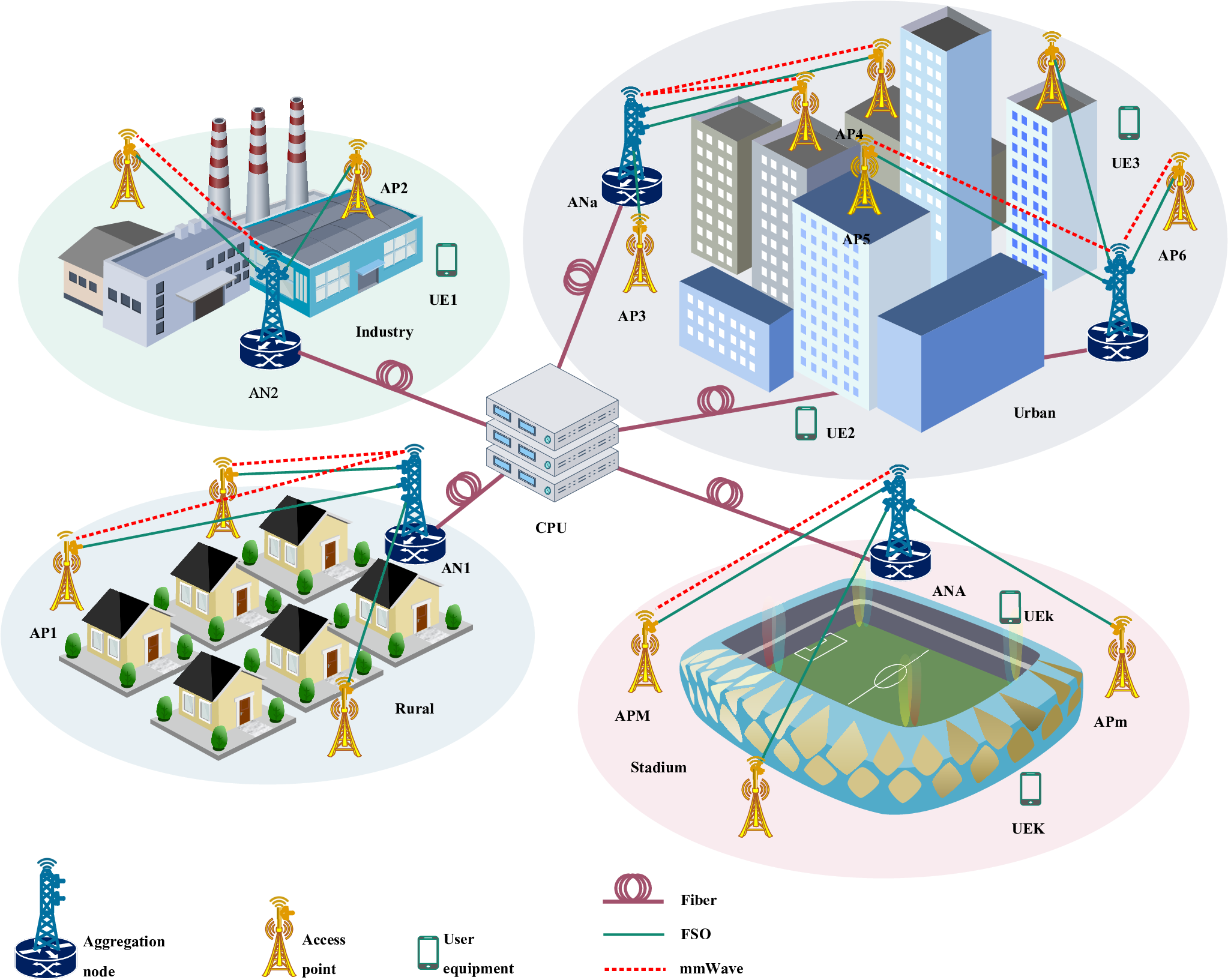
We consider a distributed mMIMO network wherein MM number of NN-antenna APs simultaneously serve KK single-antenna UEs at the same time–frequency resources. The users are distributed over a wide area with different regions, e.g., urban and rural areas, industrial estates, and crowded places, c.f. Fig. 1. To cover the whole area, it is also assumed that there exists AA ANs to gather data from all the APs via RF–FSO links, namely the fronthaul links. Every AP is equipped with a single RF fronthaul antenna and an FSO aperture for sending signals to the serving AN. Ultimately, each AN re-transmits its received signals to the CPU via a multi-core fiber (MCF) link, called the backhaul link. To analyze the performance of the proposed network, we consider two setups; (a) cell-free network and (b) user-centric one. Despite the cell-free setup in which an AP serves all UEs, for the user-centric case, each AP only serves a portion of its adjacent UEs. Moreover, to acquire channel state information (CSI), each coherence time interval is divided into two phases; uplink channel training and data transmission, where UE–AP access and AP–AN fronthaul links are estimated at the APs and ANs, respectively.
Refer to caption
(a)
Fig. 1: The mMIMO network with RF–FSO fronthauls and MCF backhauls.
Refer to caption
Fig. 2: The signal flow over access and cognitively-assigned fronthaul links.

Before investigating achievable data rates and optimization problems, we study data flow and provide channel and hardware models in the following subsections.

II-A Fronthaul Signal Flow

Considering the alignment precision and weather conditions as two main factors affecting the FSO performance, each AP decides to forward the received signal over its FSO-only, RF-only, or RF–FSO fronthaul, c.f. Fig. 2, based on a cognitive fronthaul assignment algorithm. To this end, we consider four weather conditions–clear, rainy, snowy, and foggy. Also, we suggest three FSO alignment conditions–poor, moderate, and good alignments. In the case of RF-only and RF–FSO fronthauling, the available RF bandwidth is shared between the access and fronthaul links due to its high cost, and the frequency-division multiplexing (FDM) method is applied. Let us consider the RF bandwidth as BW, and define BW0\text{BW}_{0} and BWm\text{BW}_{m} as the bandwidths of the access layer and the mmth AP’s RF fronthaul, respectively. So, we have BW0=mina=1,2,…,A​{BW0a}\text{BW}_{0}\!=\!\underset{a=1,2,...,A}{\text{min}}\{\text{BW}_{0_{a}}\!\}, where BW0a=BWm=BW/(Δa+1)\text{BW}_{0_{a}}\!=\!\text{BW}_{m}\!=\!\text{BW}/(\Delta_{a}\!+\!1), m∈ℳ⁡(a)m\!\in\!\mathcal{M}(a)11 1 Since the received signals at an AP are analogy reformed and forwarded, its input and output RF signals’ bandwidths are equal. . Herein, Δa\Delta_{a} is the number of the RF links connected to the aath AN, for a=1,2,…,Aa=1,2,...,A. Thanks to beamforming and interference cancellation techniques, the fronthauls’ RF bandwidths are reused per AN. Besides, ℳ⁡(a)\mathcal{M}(a) denotes the set of the APs served by the aath AN, where ∑a=1Aℳ⁡(a)=M\sum_{a=1}^{A}\mathcal{M}(a)\!=\!M, and ℳ⁡(a)∩ℳ⁡(a′)=∅\mathcal{M}(a)\cap\mathcal{M}(a^{\prime})\!=\!\varnothing if a≠a′a\neq a^{\prime}.

II-B Access Channels

The RF access link between the kkth UE and mmth AP is modeled as

𝐠m​k=βm​k1/2𝐡m​k, for m=1,2,…,M and k=1,2,…,K,\mathbf{g}_{mk}=\beta_{mk}^{1/2}\mathbf{h}_{mk},\text{~for~}m=1,2,...,M\text{~and~}k=1,2,...,K, (1)

where βm​k\beta_{mk} denotes the large-scale fading, and 𝐡m​k∈ℂN×1\mathbf{h}_{mk}\!\in\!\mathbb{C}^{N\times 1} represents the small-scale Rayleigh fading coefficients such that its elements are independent and identically distributed (i.i.d.) 𝒞​𝒩​(0,1)\mathcal{CN}(0,1) RVs.

II-C Fronthaul Channels

Since the fronthaul link could be FSO-only, RF-only, or RF–FSO, in what follows, we discuss channel modelings of RF and FSO links.

II-C1 RF links

For the case of RF link between the mmth AP and aath AN, we have

Ia​mRF=βa​m1/2​ha​m, for ​m∈ℳ⁡(a),I_{am}^{\text{RF}}=\beta_{am}^{1/2}h_{am},\text{~for~}m\!\in\!\mathcal{M}(a), (2)

where βa​m\beta_{am} and ha​mh_{am} respectively present the large-scale and the small-scale fading terms.

II-C2 FSO links

For the case of FSO fronthaul, we have

Ia​mFSO=Il,a​m​It,a​m​Ip,a​m, for ​m∈ℳ⁡(a),I_{am}^{\text{FSO}}=I_{l,am}I_{t,am}I_{p,am},\text{~for~}m\!\in\!\mathcal{M}(a), (3)

where Il,a​mI_{l,am} denotes the path-loss [33]

Il,a​m=Ar​e−γ​da​m(ϕr​da​m)2:=Il,a​m′​e−γ​da​m,I_{l,am}=\frac{A_{r}e^{-\gamma d_{am}}}{(\phi_{r}d_{am})^{2}}:=I_{l,am}^{\prime}e^{-\gamma d_{am}}, (4)

where ArA_{r}, da​md_{am}, ϕr\phi_{r}, and γ\gamma denote aperture area, fronthaul length, beam divergence angle, and weather-dependent attenuation coefficient, respectively. Besides, It,a​mI_{t,am} is the atmospheric turbulence-induced fading, modeled via a log-normal distribution with the following probability distribution function (p.d.f) of [24]

fIt,a​m​(It,a​m)=\displaystyle f_{I_{t,am}}(I_{t,am})=
12​It,a​m​2​π​δl,a​m2​exp⁡(−(ln⁡(It,a​m)+2​δl,a​m2)28​δl,a​m2),\displaystyle~~~\frac{1}{2I_{t,am}\sqrt{2\pi\delta_{l,am}^{2}}}\,\operatorname{exp}\!\left(\!\!-\frac{{\left(\ln(I_{t,am})+2\delta_{l,am}^{2}\right)^{2}}}{8\delta_{l,am}^{2}}\!\right)\!\!, (5)

where δl,a​m2=0.307​Cn2​ka​m7/6​da​m11/6\delta_{l,am}^{2}\!=\!0.307C_{n}^{2}k_{am}^{7/6}d_{am}^{11/6} is the log-amplitude variance for plane waves, and Cn2C_{n}^{2} denotes the index of refraction structure parameter. Herein, ka​m=2​π/λa​mk_{am}\!=\!{2\pi}/\lambda_{am} in which λa​m\lambda_{am} is the wavelength of the FSO link. Furthermore, Ip,a​mI_{p,am} represents the boresight pointing error with the following pdf [34]

fIp,a​m​(Ip,a​m)=ξ2I0ξ2​Ip,a​mξ2−1,0≤Ip,a​m≤I0,f_{I_{p,am}}(I_{p,am})=\frac{\xi^{2}}{I_{0}^{\xi^{2}}}I_{p,am}^{\xi^{2}-1},~~0\leq I_{p,am}\leq I_{0}, (6)

where I0=[erf⁡(v)]2I_{0}\!=\!\left[\operatorname{erf}(v)\right]^{2}, and ξ=12​wze​q​σs−1\xi\!=\!\frac{1}{2}w_{z_{eq}}\sigma_{s}^{-1} implies the ratio of the equivalent beam radius to the pointing error displacement standard deviation at the receiver. Moreover, wze​q2=wz2​0.25​π​erf⁡(v)​v−1​exp⁡(v2)w_{z_{eq}}^{2}\!=\!w_{z}^{2}\sqrt{0.25\pi}\operatorname{erf}(v)v^{-1}\operatorname{exp}(v^{2}) and v=0.5​π​wz−1​rsv\!=\!\sqrt{0.5\pi}w_{z}^{-1}r_{s}, where wzw_{z} is the beam waist at distance zz, and rsr_{s} depicts the alignment-based radial distance at the detector. Finally, the pdf of the Ia​mFSOI_{am}^{\text{FSO}} is obtained as [34]

fIa​mFSO​(Ia​mFSO)=ξ2​(Ia​mFSO)ξ2−12​(I0​Il,a​m)ξ2​erfc⁡(ln⁡(Ia​mFSOI0​Il,a​m)+φa​m8​δl,a​m2)​φa​m′,f_{I_{am}^{\text{FSO}}}(I_{am}^{\text{FSO}})=\frac{\xi^{2}(I_{am}^{\text{FSO}})^{\xi^{2}-1}}{2(I_{0}I_{l,am})^{\xi^{2}}}\operatorname{erfc}\!\left(\!\frac{\ln\!\left(\!{\dfrac{I_{am}^{\text{FSO}}}{I_{0}I_{l,am}}}\!\right)\!+\!\varphi_{am}}{\sqrt{8\delta_{l,am}^{2}}}\!\right)\!\varphi_{am}^{\prime}, (7)

where φa​m=2​δl,a​m2​(1+2​ξ2)\varphi_{am}\!=\!2\delta_{l,am}^{2}\!\left(1+2\xi^{2}\right) and φa​m′=2​δl,a​m2​ξ2​(1+ξ2)\varphi_{am}^{\prime}\!=\!2\delta_{l,am}^{2}\xi^{2}\!\left(1+\xi^{2}\right).

II-D Hardware Models

The received signals at the APs and ANs are analogy reformed and forwarded through the fronthaul and backhaul links, respectively. Two hardware models are employed; clipping and HI models. In general, the noisy distorted signal is modeled by the Bussgang theorem, as follows [35]

xo​u​t=μ​xi​n+nd,x_{out}=\mu x_{in}+n_{d}, (8)

where μ∈{μm,μa}\mu\!\in\!\{\mu_{m},\mu_{a}\} denotes the distortion gain. Furthermore, xi​n∼𝒞​𝒩​(0,δ2)x_{in}\!\sim\!\mathcal{CN}(0,\delta^{2}) is input signal, and nd∼𝒞​𝒩​(0,δd2)n_{d}\!\sim\!\mathcal{CN}(0,\delta_{d}^{2}) is the distortion noise.

II-D1 Clipping Model

To convert the RF signals to the FSO form at an AP, we apply a clipping model in which the received signal is firstly clipped, and then a DC bias is added to make the optical signal non-negative. Finally, the amplified signal is transmitted with a laser diode. This technique is called RF-over-FSO (RoFSO), c.f. Fig. 3 (a). Likewise, the same method is used for reforming the FSO and/or RF signals to match the fiber optics at an AN, sequentially named RF-over-fiber (RoF) and FSO-over-fiber (FSoF), c.f. Fig. 3 (b). For the clipping model, the distortion gain becomes [24]

μ=μ0​erf⁡(Bc2​μ02​δ2),\mu=\mu_{0}\,{\operatorname{erf}}\!\left(\!\frac{B_{c}}{\sqrt{2\mu_{0}^{2}\delta^{2}}}\!\right)\!, (9)

where μ0\mu_{0} denotes the laser’s gain, BcB_{c} represents the clipping level, and the variance of the distortion noise is given by [24]

δd2\displaystyle\delta_{d}^{2} =Bc2​(2−μμ0)+μ02​δ2​(1−μμ0)​μμ0\displaystyle=B_{c}^{2}\Big(2-\dfrac{\mu}{\mu_{0}}\Big)+\mu_{0}^{2}\delta^{2}\Big(1-\dfrac{\mu}{\mu_{0}}\Big)\dfrac{\mu}{\mu_{0}}
−2​Bc2​μ02​δ2π​exp⁡(−Bc22​μ02​δ2).\displaystyle~~~-\sqrt{\frac{2B_{c}^{2}\mu_{0}^{2}\delta^{2}}{\pi}}\,{\operatorname{exp}}\!\left(\!-{\frac{B_{c}^{2}}{2\mu_{0}^{2}\delta^{2}}}\!\right)\!\!. (10)
Refer to caption
(a)
Refer to caption
(b)
Fig. 3: The simplified hardware models at the (a) APs and (b) ANs. Here, IF stands for intermediate frequency and BB indicates baseband.

II-D2 Hardware Impairment Model

Since the RF devices and signal processing are not ideal, the up-conversion of the received RF signals at an AP and forwarding them over the RF fronthaul links are subject to the HI, which is named RF-over-RF (RoR), as shown in Fig. 3 (a). In (8), we set μ=ξ1/2\mu\!=\!\xi^{1/2}, where ξ∈[0,1]\xi\!\in\![0,1] indicates the hardware quality factor, nd∼𝒞​𝒩​(0,(1−ξ)​δ2)n_{d}\!\sim\!\mathcal{CN}(0,(1-\xi)\delta^{2}) is uncorrelated with the input signal, and we have 𝔼⁡{|xo​u​t|2}=𝔼⁡{|xi​n|2}=δ2\mathbb{E}\left\{|x_{out}|^{2}\right\}\!=\!\mathbb{E}\left\{|x_{in}|^{2}\right\}\!=\!\delta^{2} [12].

III Channel Training and Data Transmission

In this section, we firstly present the uplink channel training phase to estimate the RF and FSO channel coefficients. Then, the uplink data transmissions are investigated.

III-A Uplink Channel Training

In the channel training phase, the UEs and APs independently transmit channel training sequences through their access and fronthaul links, respectively. The channel coefficients of the RF access links are estimated at each AP after some mathematical computations. Likewise, the channel gains of the RF and FSO fronthaul links are acquired at the corresponding ANs. Without loss of generality, it is assumed that the CPU knows the estimated channels derived at the APs and ANs. Likewise, the estimated channels at each AN are shared with the served APs, which is required for the fronthaul assignment algorithm.

III-A1 RF channel estimation at APs

All UEs transmit their τp\tau_{p}-length mutually orthogonal pilot sequences τp​ρp​𝝋k∈ℂτp×1\sqrt{\tau_{p}\rho_{p}}\bm{\varphi}_{k}\!\in\!\mathbb{C}^{\tau_{p}\times 1} for k=1,2,…,Kk=1,2,...,K, where ‖𝝋k‖2=1||\bm{\varphi}_{k}||^{2}\!=\!1 and τp≥K\tau_{p}\!\geq\!K. Therefore, the N×τpN\!\times\!\tau_{p} received superimposed pilot matrix at the mmth AP is given by

𝒚p,m=τp​ρp​∑k=1K𝐠m​k​𝝋kH+𝝎p,m,\bm{y}_{p,m}=\sqrt{\tau_{p}\rho_{p}}\sum\limits_{k=1}^{K}\mathbf{g}_{mk}\bm{\varphi}_{k}^{H}+\bm{\omega}_{p,m}, (11)

where ρp\rho_{p} represents pilot transmission power, and 𝝎p,m∼𝒞​𝒩​(0,σp,m2​IN)\bm{\omega}_{p,m}\!\sim\!\mathcal{CN}(0,\sigma_{p,m}^{2}\mathbf{\textit{I}}_{N}) denotes the additive noise matrix with i.i.d. elements. Afterward, the received signal is multiplied with the conjugate transpose of the kkth UE’s pilot sequence as

𝒚~p,m​k=𝒚p,m​𝝋k=τp​ρp​∑k′=1K𝐠m​k′​𝝋k′H​𝝋k+𝝎p,m​𝝋k.\tilde{\bm{y}}_{p,mk}=\bm{y}_{p,m}\bm{\varphi}_{k}=\sqrt{\tau_{p}\rho_{p}}\sum\limits_{k^{\prime}=1}^{K}\mathbf{g}_{mk^{\prime}}\bm{\varphi}_{k^{\prime}}^{H}\bm{\varphi}_{k}+\bm{\omega}_{p,m}\bm{\varphi}_{k}. (12)

To obtain the wireless channel coefficients at the mmth AP, a linear minimum mean-square error (LMMSE) estimation is performed as follows

𝐠^m​k\displaystyle\hat{\mathbf{g}}_{mk} =(𝔼⁡{𝐠m​k​𝒚~p,m​kH})​(𝔼⁡{𝒚~p,m​k​𝒚~p,m​kH})−1​𝒚~p,m​k\displaystyle=\Big({\mathbb{E}\big\{\mathbf{g}_{mk}\tilde{\bm{y}}_{p,mk}^{H}\!\big\}}\!\Big)\!\Big({\mathbb{E}\big\{\tilde{\bm{y}}_{p,mk}\tilde{\bm{y}}_{p,mk}^{H}\!\big\}}\!\Big)^{\!-1}\tilde{\bm{y}}_{p,mk}
=τp​ρp​βm​kτp​ρp​∑k′=1Kβm​k′​|𝝋k′H​𝝋k|2+σp,m2​𝒚~p,m​k:=ζm​k​𝒚~p,m​k,\displaystyle=\frac{\sqrt{\tau_{p}\rho_{p}}\beta_{mk}}{{\tau_{p}\rho_{p}}\sum\limits_{k^{\prime}=1}^{K}\beta_{mk^{\prime}}|\bm{\varphi}_{k^{\prime}}^{H}\bm{\varphi}_{k}|^{2}+\sigma_{p,m}^{2}}\tilde{\bm{y}}_{p,mk}:=\zeta_{mk}\tilde{\bm{y}}_{p,mk}, (13)

and the mean-square of the estimated channel becomes

γm​k\displaystyle\gamma_{mk} =:𝔼⁡{𝐠^m​kH​𝐠^m​k}=τp​ρp​βm​k​ζm​k.\displaystyle=:\mathbb{E}\{\hat{\mathbf{g}}_{mk}^{H}\hat{\mathbf{g}}_{mk}\}=\sqrt{\tau_{p}\rho_{p}}\beta_{mk}\zeta_{mk}. (14)

III-A2 FSO channel estimation at ANs

To measure the FSO channel gain between the aath AN and the served mmth AP, the AP sends its τp\tau_{p}-length mutually orthogonal pilot signal 𝝋m\bm{\varphi}_{m} through its FSO link, where ‖𝝋m‖2=1||\bm{\varphi}_{m}||^{2}\!=\!1. Thus, the received signal at the aath AN is modeled as22 2 We assume that the FSO detectors are sufficiently spaced to avoid optical interference and cross-talk [22].

𝒚p,a​m=τp​PmaxFSO​Ia​mFSO​𝝋m+𝝊p,a​m,\bm{y}_{p,am}=\sqrt{\tau_{p}P_{\text{max}}^{\text{FSO}}}I_{am}^{\text{FSO}}\bm{\varphi}_{m}+\bm{\upsilon}_{p,am}, (15)

where PmaxFSOP_{\text{max}}^{\text{FSO}} is the maximum FSO transmission power at each AP satisfying the eye-safety regulations, and 𝝊p,a​m∼𝒞​𝒩​(0,(ϕp,a​mFSO)2​Iτp)\bm{\upsilon}_{p,am}\!\sim\!\mathcal{CN}(0,(\phi_{p,am}^{\text{FSO}})^{2}\mathbf{\textit{I}}_{\tau_{p}}) is the additive noise vector with i.i.d. elements. Similarly, by multiplying 𝒚p,a​m\bm{y}_{p,am} with 𝝋mH\bm{\varphi}_{m}^{H}, and applying the LMMSE33 3 The LMMSE is a sub-optimal estimation technique for the FSO channels due to their non-Gaussian statistics., we have

I^a​mFSO=τp​PmaxFSO​Γa​m2τp​PmaxFSO​Γa​m2+(ϕp,a​mFSO)2​y~p,a​m:=ζa​mFSO​y~p,a​m,\hat{I}_{am}^{\text{FSO}}=\frac{\sqrt{\tau_{p}P_{\text{max}}^{\text{FSO}}}\,\Gamma_{am}^{2}}{{\tau_{p}P_{\text{max}}^{\text{FSO}}}\Gamma_{am}^{2}+(\phi_{p,am}^{\text{FSO}})^{2}}\tilde{{y}}_{p,am}:=\zeta_{am}^{\text{FSO}}\tilde{{y}}_{p,am}, (16)

where, by use of (7), Γa​mn\Gamma_{am}^{n} is

Γa​mn\displaystyle\Gamma_{am}^{n} =:𝔼⁡{|Ia​mFSO|n}=ξ2​(I0​Il,a​m)nξ2+n\displaystyle=:\mathbb{E}\{|I_{am}^{\text{FSO}}|^{n}\}=\frac{\xi^{2}(I_{0}I_{l,am})^{n}}{\xi^{2}+n}
×exp⁡[2​(ξ2+n)2​δl,a​m2−(ξ2+n)​φa​m]​φa​m′,\displaystyle~~~\times\!\operatorname{exp}\!\bigg[2\Big(\xi^{2}\!+\!n\Big)^{\!2}\delta_{l,am}^{2}\!-\!\Big(\xi^{2}\!+\!n\Big)\varphi_{am}\bigg]\varphi_{am}^{\prime}, (17)

and the mean-square of the estimated channel becomes

γa​mFSO\displaystyle\gamma_{am}^{\text{FSO}} =:𝔼⁡{|I^a​mFSO|2}=τp​PmaxFSO​Γa​m2​ζa​mFSO.\displaystyle=:\mathbb{E}\{|\hat{I}_{am}^{\text{FSO}}|^{2}\}=\sqrt{\tau_{p}P_{\text{max}}^{\text{FSO}}}\,\Gamma_{am}^{2}\zeta_{am}^{\text{FSO}}. (18)

III-A3 RF channel estimation at ANs

The mmth AP transmits τp\tau_{p}-length mutually orthogonal pilot sequence 𝝋m′\bm{\varphi}_{m}^{\prime} to the serving AN via its RF link. Hence, the τp×1\tau_{p}\!\times\!1 received pilot vector at the aath AN is given by

𝒚p,a​m′=τp​PmaxRF​Ia​mRF​𝝋m′+𝝊p,a​m′,\bm{y}_{p,am}^{\prime}=\sqrt{\tau_{p}P_{\text{max}}^{\text{RF}}}I_{am}^{\text{RF}}\bm{\varphi}_{m}^{\prime}+\bm{\upsilon}_{p,am}^{\prime}, (19)

where PmaxRFP_{\text{max}}^{\text{RF}} denotes the maximum wireless transmission power at each AP, and 𝝊p,a​m′∼𝒞​𝒩​(0,(ϕp,a​mRF)2​Iτp)\bm{\upsilon}_{p,am}^{\prime}\!\sim\!\mathcal{CN}(0,(\phi_{p,am}^{\text{RF}})^{2}\mathbf{\textit{I}}_{\tau_{p}}) represents the additive noise vector with i.i.d. components. Since ‖𝝋m′‖2=1||\bm{\varphi}_{m}^{\prime}||^{2}\!=\!1, by multiplying 𝒚p,a​m′\bm{y}_{p,am}^{\prime} with 𝝋m′H\bm{\varphi}_{m}^{\prime H}, and applying the LMMSE, we have

I^a​mRF=τp​PmaxRF​βa​mτp​PmaxRF​βa​m+(ϕp,a​mRF)2​y~p,a​m′:=ζa​mRF​y~p,a​m′,\hat{I}_{am}^{\text{RF}}=\frac{\sqrt{\tau_{p}P_{\text{max}}^{\text{RF}}}\,\beta_{am}}{{\tau_{p}P_{\text{max}}^{\text{RF}}}\beta_{am}+(\phi_{p,am}^{\text{RF}})^{2}}\tilde{{y}}_{p,am}^{\prime}:=\zeta_{am}^{\text{RF}}\tilde{{y}}_{p,am}^{\prime}, (20)

and the mean-square of the estimated channel is derived as

γa​mRF\displaystyle\gamma_{am}^{\text{RF}} =:𝔼⁡{|I^a​mRF|2}=τp​PmaxRF​βa​m​ζa​mRF.\displaystyle=:\mathbb{E}\{|\hat{I}_{am}^{\text{RF}}|^{2}\}=\sqrt{\tau_{p}P_{\text{max}}^{\text{RF}}}\,\beta_{am}\zeta_{am}^{\text{RF}}. (21)

III-B Uplink Data Transmission

After receiving the UEs’ data signal in the uplink by each AP, it reforms and forwards the processed signal over its fronthaul to the dedicated AN. Then, the corresponding AN reshapes the received FSO and/or RF signals to the optical ones and delivers them to the CPU via its MCF backhaul link. Finally, users’ data recovery is performed at the CPU. In what follows, the details of data recovery are presented.

III-B1 User-centric clustering

In the UC-mMIMO network [8], the mmth AP only supports a subset of all UEs, i.e., 𝒦⁡(m)⊆{1,2,…,K}\mathcal{K}(m)\!\subseteq\!\{1,2,...,K\}. Consequently, ℳ⁡(k)\mathcal{M}(k) denotes the set of APs serving the kkth UE, which is defined as ℳ⁡(k)={m:k∈𝒦⁡(m)}.\mathcal{M}(k)=\left\{m:k\in\mathcal{K}(m)\right\}\!. By applying a neighborhood clustering mechanism [7], the mmth AP classifies the estimated channel coefficients in a descending order and only serves a limited number of UEs, i.e., |𝒦⁡(m)|≤K|\mathcal{K}(m)|\!\leq\!K.

III-B2 Data processing at APs

First, the received signal at the mmth AP is given by

𝒚u,m=ρu​∑k=1Kηk​𝐠m​k​sk+𝝎u,m,\bm{y}_{u,m}=\sqrt{\rho_{u}}\sum\limits_{k=1}^{K}\sqrt{\eta_{k}}\mathbf{g}_{mk}s_{k}+\bm{\omega}_{u,m}, (22)

where sk∼𝒞​𝒩​(0,1)s_{k}\!\sim\!\mathcal{CN}(0,1) denotes the information symbol of the kkth UE weighted by power control coefficient ηk∈[0,1]\eta_{k}\!\in\![0,1]. Also, ρu\rho_{u} represents the maximum signal transmission power, and 𝝎u,m∼𝒞​𝒩​(0,σu,m2​IN)\bm{\omega}_{u,m}\!\sim\!\mathcal{CN}(0,\sigma_{u,m}^{2}\mathbf{\textit{I}}_{N}) indicates the additive noise vector with i.i.d. elements. Then, the received signal is reformed using the RoFSO and/or RoR techniques and forwarded through FSO and/or RF fronthaul links, respectively, as follows

𝒙~u,a​m=ϵa​m​(μm​𝒚u,m+𝒏d,m):=ϵa​m​𝒙u,a​m,\tilde{\bm{x}}_{u,am}=\epsilon_{am}\Big(\mu_{m}\bm{y}_{u,m}+\bm{n}_{d,m}\!\Big):=\epsilon_{am}{\bm{x}}_{u,am}, (23)
𝒙~u,a​m′=ϵa​m′​(μm′​𝒚u,m+𝒏d,m′):=ϵa​m′​𝒙u,a​m′,\tilde{\bm{x}}_{u,am}^{\prime}=\epsilon_{am}^{\prime}\Big(\mu_{m}^{\prime}\bm{y}_{u,m}+\bm{n}_{d,m}^{\prime}\!\Big):=\epsilon_{am}^{\prime}{\bm{x}}_{u,am}^{\prime}, (24)

where μm\mu_{m} and μm′\mu_{m}^{\prime} denote the FSO and RF distortion gains, respectively. Herein, 𝒏d,m∼𝒞​𝒩​(0,δd,m2​IN)\bm{n}_{d,m}\!\sim\!\mathcal{CN}(0,\delta_{d,m}^{2}\mathbf{\textit{I}}_{N}) and 𝒏d,m′∼𝒞​𝒩​(0,δd,m′2​IN)\bm{n}_{d,m}^{\prime}\!\sim\!\mathcal{CN}(0,\delta_{d,m}^{\prime 2}\mathbf{\textit{I}}_{N}) represent the distortion noises. In addition, ϵa​m∈{0,1}\epsilon_{am}\!\in\!\{0,1\} and ϵa​m′∈{0,1}\epsilon_{am}^{\prime}\!\in\!\{0,1\} present the fronthaul assignment indices of the FSO and RF links between the aath AN and the mmth AP, m∈ℳ⁡(a)m\!\in\!\mathcal{M}(a), respectively. With ϵa​m=1\epsilon_{am}\!=\!1 and ϵa​m′=0\epsilon_{am}^{\prime}\!=\!0, the signal is sent over the FSO-only fronthaul, while with ϵa​m=0\epsilon_{am}\!=\!0 and ϵa​m′=1\epsilon_{am}^{\prime}\!=\!1, the signal is sent through the RF-only fronthaul. However, the signal is transmitted over the RF–FSO fronthaul if ϵa​m=ϵa​m′=1\epsilon_{am}\!=\!\epsilon_{am}^{\prime}\!=\!1.

III-B3 Data processing at ANs

The received FSO and/or RF signals at the aath AN are sequentially presented as below

𝒚u,a​m=ϵa​m​(𝒙u,a​m​Ia​mFSO+𝝊u,a​m),\bm{y}_{u,am}=\epsilon_{am}\Big({\bm{x}}_{u,am}I_{am}^{\text{FSO}}+\bm{\upsilon}_{u,am}\!\Big), (25)
𝒚u,a​m′=ϵa​m′​(𝒙u,a​m′​Ia​mRF+𝝊u,a​m′),\bm{y}_{u,am}^{\prime}=\epsilon_{am}^{\prime}\Big({\bm{x}}_{u,am}^{\prime}I_{am}^{\text{RF}}+\bm{\upsilon}_{u,am}^{\prime}\!\Big), (26)

Also, 𝝊u,a​m∼𝒞​𝒩​(0,(ϕu,a​mFSO)2​IN)\bm{\upsilon}_{u,am}\!\sim\!\mathcal{CN}(0,(\phi_{u,am}^{\text{FSO}})^{2}\mathbf{\textit{I}}_{N}) and 𝝊u,a​m′∼𝒞​𝒩​(0,(ϕu,a​mRF)2​IN)\bm{\upsilon}_{u,am}^{\prime}\!\sim\!\mathcal{CN}(0,(\phi_{u,am}^{\text{RF}})^{2}\mathbf{\textit{I}}_{N}) are the additive noise vectors at the AN with i.i.d. elements. Then, the AN applies the FSoF and RoF techniques to match the FSO and/or RF signals with the optical forms, respectively, and sends them over the connected MCF backhaul link.

III-B4 Data processing at the CPU

The CPU acquires the reshaped and noisy versions of the FSO and/or RF signal vectors sequentially as below

𝒓u,a​m=μa​m​𝒚u,a​m+ϵa​m​(𝒏d,a​m+𝝂CPU),\bm{r}_{u,am}=\mu_{am}\bm{y}_{u,am}+\epsilon_{am}\Big(\bm{n}_{d,am}+\bm{\nu}_{\text{CPU}}\!\Big), (27)
𝒓u,a​m′=μa​m′​𝒚u,a​m′+ϵa​m′​(𝒏d,a​m′+𝝂CPU),\bm{r}_{u,am}^{\prime}=\mu_{am}^{\prime}\bm{y}_{u,am}^{\prime}+\epsilon_{am}^{\prime}\Big(\bm{n}_{d,am}^{\prime}+\bm{\nu}_{\text{CPU}}\!\Big), (28)

where μa​m\mu_{am} and μa​m′\mu_{am}^{\prime} represent the FSO and RF distortion gains, respectively. Also, 𝒏d,a​m∼𝒞​𝒩​(0,δd,a​m2​IN)\bm{n}_{d,am}\!\sim\!\mathcal{CN}(0,\delta_{d,am}^{2}\mathbf{\textit{I}}_{N}) and 𝒏d,a​m′∼𝒞​𝒩​(0,δd,a​m′2​IN)\bm{n}_{d,am}^{\prime}\!\sim\!\mathcal{CN}(0,\delta_{d,am}^{\prime 2}\mathbf{\textit{I}}_{N}) illustrate the distortion noises, and 𝝂CPU∼𝒞​𝒩​(0,ϕCPU2​IN)\bm{\nu}_{\text{CPU}}\!\sim\!\mathcal{CN}(0,\phi_{\text{CPU}}^{2}\mathbf{\textit{I}}_{N}) denotes the additive noise at the CPU. By using (22)–(28), the received signals at the CPU are rewritten as

𝒓u,a​m=ϵa​m​(Ja​m​Ia​mFSO​∑k=1Kηk​𝐠m​k​sk+𝚯u,a​m),\bm{r}_{u,am}=\epsilon_{am}\bigg(\!J_{am}I_{am}^{\text{FSO}}\sum\limits_{k=1}^{K}\sqrt{\eta_{k}}\mathbf{g}_{mk}s_{k}+\bm{\Theta}_{u,am}\!\bigg), (29)
𝒓u,a​m′=ϵa​m′​(Ja​m′​Ia​mRF​∑k=1Kηk​𝐠m​k​sk+𝚯u,a​m′),\bm{r}_{u,am}^{\prime}=\epsilon_{am}^{\prime}\bigg(\!J_{am}^{\prime}I_{am}^{\text{RF}}\sum\limits_{k=1}^{K}\sqrt{\eta_{k}}\mathbf{g}_{mk}s_{k}+\bm{\Theta}_{u,am}^{\prime}\!\bigg), (30)

where Ja​m=ρu​μm​μa​mJ_{am}\!=\!\sqrt{\rho_{u}}\mu_{m}\mu_{am}, Ja​m′=ρu​μm′​μa​m′J_{am}^{\prime}\!=\!\sqrt{\rho_{u}}\mu_{m}^{\prime}\mu_{am}^{\prime}, and we have

𝚯u,a​m\displaystyle\bm{\Theta}_{u,am} =μm​μa​m​Ia​mFSO​𝝎u,m+μa​m​Ia​mFSO​𝒏d,m\displaystyle=\mu_{m}\mu_{am}I_{am}^{\text{FSO}}\bm{\omega}_{u,m}+\mu_{am}I_{am}^{\text{FSO}}\bm{n}_{d,m}
+μa​m​𝝊u,a​m+𝒏d,a​m+𝝂CPU,\displaystyle~~~+\mu_{am}\bm{\upsilon}_{u,am}+\bm{n}_{d,am}+\bm{\nu}_{\text{CPU}},
𝚯u,a​m′\displaystyle\bm{\Theta}_{u,am}^{\prime} =μm′​μa​m′​Ia​mRF​𝝎u,m+μa​m′​Ia​mRF​𝒏d,m′\displaystyle=\mu_{m}^{\prime}\mu_{am}^{\prime}I_{am}^{\text{RF}}\bm{\omega}_{u,m}+\mu_{am}^{\prime}I_{am}^{\text{RF}}\bm{n}_{d,m}^{\prime}
+μa​m′​𝝊u,a​m′+𝒏d,a​m′+𝝂CPU,\displaystyle~~~+\mu_{am}^{\prime}\bm{\upsilon}_{u,am}^{\prime}+\bm{n}_{d,am}^{\prime}+\bm{\nu}_{\text{CPU}},

where 𝔼⁡{𝚯u,a​m}=𝔼⁡{𝚯u,a​m′}=0\mathbb{E}\{\bm{\Theta}_{u,am}\}\!=\!\mathbb{E}\{\bm{\Theta}_{u,am}^{\prime}\}\!=\!0. Besides, the covariance matrices of 𝚯u,a​m\bm{\Theta}_{u,am} and 𝚯u,a​m′\bm{\Theta}_{u,am}^{\prime} are respectively denoted by 𝛀u,a​m2=Ωu,a​m2​IN×N\bm{\Omega}_{u,am}^{2}\!=\!{\Omega}_{u,am}^{2}\mathbf{\textit{I}}_{N\!\times\!N} and 𝛀u,a​m′2=Ωu,a​m′2​IN×N\bm{\Omega}_{u,am}^{\prime 2}\!=\!{\Omega}_{u,am}^{\prime 2}\mathbf{\textit{I}}_{N\!\times\!N}, where

Ωu,a​m2\displaystyle{\Omega}_{u,am}^{2} =μm2​μa​m2​Γa​m2​σu,m2+μa​m2​Γa​m2​δd,m2\displaystyle=\mu_{m}^{2}\mu_{am}^{2}\Gamma_{am}^{2}\sigma_{u,m}^{2}+\mu_{am}^{2}\Gamma_{am}^{2}\delta_{d,m}^{2}
+μa​m2​(ϕu,a​mFSO)2+δd,a​m2+ϕCPU2,\displaystyle~~~+\mu_{am}^{2}(\phi_{u,am}^{\text{FSO}})^{2}+\delta_{d,am}^{2}+\phi_{\text{CPU}}^{2}, (31)
Ωu,a​m′2\displaystyle{\Omega}_{u,am}^{\prime 2} =μm′2​μa​m′2​βa​m​σu,m2+μa​m′2​βa​m​δd,m′2\displaystyle=\mu_{m}^{\prime 2}\mu_{am}^{\prime 2}\beta_{am}\sigma_{u,m}^{2}+\mu_{am}^{\prime 2}\beta_{am}\delta_{d,m}^{\prime 2}
+μa​m′2​(ϕu,a​mRF)2+δd,a​m′2+ϕCPU2.\displaystyle~~~+\mu_{am}^{\prime 2}(\phi_{u,am}^{\text{RF}})^{2}+\delta_{d,am}^{\prime 2}+\phi_{\text{CPU}}^{2}. (32)

One can show that all terms of the overall additive noises are mutually uncorrelated. Thus, the variances of the noises, given in (III-B4) and (III-B4), become equal to the sum of the variances of superimposed noises.

IV Achievable Rates Analysis

The data recovery and uplink achievable data rates, for the CF- and UC-mMIMO networks, are discussed in the following subsections.

IV-A Uplink Data Recovery

By applying the MRC detection at the CPU, data recovery is performed for the CF- and UC-mMIMO networks.

IV-A1 UC-mMIMO network

The CPU gathers the uplink signals from AA ANs, i.e., (29) and (30), and recovers the data symbol of the kkth UE, i.e. sks_{k}, by applying the following MRC technique

ru,k=∑a=1A∑m∈ℳk​(a)𝐠^m​kH​((I^a​mFSO)∗​𝒓u,a​m+(I^a​mRF)∗​𝒓u,a​m′),\displaystyle r_{u,k}=\!\sum\limits_{a=1}^{A}\sum\limits_{m\in\mathcal{M}_{k}(a)}\!\!\!\!\hat{\mathbf{g}}_{mk}^{H}\Big(\!(\hat{I}_{am}^{\text{FSO}})^{*}\bm{r}_{u,am}\!+\!(\hat{I}_{am}^{\text{RF}})^{*}\bm{r}_{u,am}^{\prime}\!\Big)\!, (33)

where ℳk​(a)=ℳ⁡(a)∩ℳ⁡(k)\mathcal{M}_{k}(a)\!=\!\mathcal{M}(a)\cap\mathcal{M}(k).

IV-A2 CF-mMIMO network

For the CF-mMIMO network, the data recovery is employed as in (33), only by use of ℳk​(a)=ℳ​(a)\mathcal{M}_{k}(a)\!=\!\mathcal{M}(a).

IV-B Uplink Achievable Data Rates

Through this subsection, we derive the uplink achievable data rates for the CF- and UC-mMIMO networks by employing the well-known use-and-then-forget (UatF) bounding technique [2].

IV-B1 UC-mMIMO network

In the UC-mMIMO network, (33) is rewritten as

ru,k=DSk​sk+BUk​sk+∑k′=1k′≠kKIUIk​k′​sk′+Nk⏟Effective noise,r_{u,k}=\text{DS}_{k}s_{k}+\underbrace{\text{BU}_{k}s_{k}+\sum\limits_{\begin{subarray}{c}k^{\prime}=1\\ k^{\prime}\neq k\end{subarray}}^{K}\text{IUI}_{kk^{\prime}}s_{k^{\prime}}+\text{N}_{k}}_{\text{Effective noise}}, (34)

where

  • •

    DSk\text{DS}_{k} denotes the desired coefficient of the kkth UE

    DSk\displaystyle\!\!\!\text{DS}_{k} =ηk𝔼{∑a=1A∑m∈ℳk​(a)ϵa​mJa​m(I^a​mFSO)∗Ia​mFSO𝐠^m​kH𝐠m​k\displaystyle=\sqrt{\eta_{k}}\,\mathbb{E}\Bigg\{\sum\limits_{a=1}^{A}\sum\limits_{m\in\mathcal{M}_{k}(a)}\!\!\epsilon_{am}J_{am}(\hat{I}_{am}^{\text{FSO}})^{*}I_{am}^{\text{FSO}}\hat{\mathbf{g}}_{mk}^{H}\mathbf{g}_{mk}
    +∑a=1A∑m∈ℳk​(a)ϵa​m′Ja​m′(I^a​mRF)∗Ia​mRF𝐠^m​kH𝐠m​k},\displaystyle~~~+\sum\limits_{a=1}^{A}\sum\limits_{m\in\mathcal{M}_{k}(a)}\!\!\epsilon_{am}^{\prime}J_{am}^{\prime}(\hat{I}_{am}^{\text{RF}})^{*}I_{am}^{\text{RF}}\hat{\mathbf{g}}_{mk}^{H}\mathbf{g}_{mk}\Bigg\}, (35)
  • •

    BUk\text{BU}_{k} is the beamforming uncertainty coefficient of the kkth UE due to the statistical knowledge of the CSI, i.e., UatF bounding,

    BUk\displaystyle\!\!\!\text{BU}_{k} =ηk​(∑a=1A∑m∈ℳk​(a)ϵa​m​Ja​m​(I^a​mFSO)∗​Ia​mFSO​𝐠^m​kH​𝐠m​kCLOSE\displaystyle=\sqrt{\eta_{k}}\Bigg(\!\sum\limits_{a=1}^{A}\sum\limits_{m\in\mathcal{M}_{k}(a)}\!\!\epsilon_{am}J_{am}(\hat{I}_{am}^{\text{FSO}})^{*}I_{am}^{\text{FSO}}\hat{\mathbf{g}}_{mk}^{H}\mathbf{g}_{mk}
    −𝔼⁡{∑a=1A∑m∈ℳk​(a)ϵa​m​Ja​m​(I^a​mFSO)∗​Ia​mFSO​𝐠^m​kH​𝐠m​k}\displaystyle-\mathbb{E}\Bigg\{\sum\limits_{a=1}^{A}\sum\limits_{m\in\mathcal{M}_{k}(a)}\!\!\epsilon_{am}J_{am}(\hat{I}_{am}^{\text{FSO}})^{*}I_{am}^{\text{FSO}}\hat{\mathbf{g}}_{mk}^{H}\mathbf{g}_{mk}\Bigg\}
    +∑a=1A∑m∈ℳk​(a)ϵa​m′Ja​m′(I^a​mRF)∗Ia​mRF𝐠^m​kH𝐠m​k\displaystyle+\sum\limits_{a=1}^{A}\sum\limits_{m\in\mathcal{M}_{k}(a)}\!\!\epsilon_{am}^{\prime}J_{am}^{\prime}(\hat{I}_{am}^{\text{RF}})^{*}I_{am}^{\text{RF}}\hat{\mathbf{g}}_{mk}^{H}\mathbf{g}_{mk}
    OPEN−𝔼⁡{∑a=1A∑m∈ℳk​(a)ϵa​m′​Ja​m′​(I^a​mRF)∗​Ia​mRF​𝐠^m​kH​𝐠m​k}),\displaystyle-\mathbb{E}\Bigg\{\sum\limits_{a=1}^{A}\sum\limits_{m\in\mathcal{M}_{k}(a)}\!\!\epsilon_{am}^{\prime}J_{am}^{\prime}(\hat{I}_{am}^{\text{RF}})^{*}I_{am}^{\text{RF}}\hat{\mathbf{g}}_{mk}^{H}\mathbf{g}_{mk}\Bigg\}\!\Bigg)\!, (36)
  • •

    IUIk​k′\text{IUI}_{kk^{\prime}} represents the inter-user interference coefficient from the k′k^{\prime}th UE

    IUIk​k′\displaystyle\!\!\!\text{IUI}_{kk^{\prime}} =ηk′​(∑a=1A∑m∈ℳk​(a)ϵa​m​Ja​m​(I^a​mFSO)∗​Ia​mFSO​𝐠^m​kH​𝐠m​k′CLOSE\displaystyle=\sqrt{\eta_{k^{\prime}}}\Bigg(\!\sum\limits_{a=1}^{A}\sum\limits_{m\in\mathcal{M}_{k}(a)}\!\!\epsilon_{am}J_{am}(\hat{I}_{am}^{\text{FSO}})^{*}I_{am}^{\text{FSO}}\hat{\mathbf{g}}_{mk}^{H}\mathbf{g}_{mk^{\prime}}
    +∑a=1A∑m∈ℳk​(a)ϵa​m′Ja​m′(I^a​mRF)∗Ia​mRF𝐠^m​kH𝐠m​k′),\displaystyle~~~+\sum\limits_{a=1}^{A}\sum\limits_{m\in\mathcal{M}_{k}(a)}\!\!\epsilon_{am}^{\prime}J_{am}^{\prime}(\hat{I}_{am}^{\text{RF}})^{*}I_{am}^{\text{RF}}\hat{\mathbf{g}}_{mk}^{H}\mathbf{g}_{mk^{\prime}}\!\Bigg)\!, (37)
  • •

    Nk\text{N}_{k} indicates the overall additive effective noises

    Nk\displaystyle\!\!\!\text{N}_{k} =∑a=1A∑m∈ℳk​(a)ϵa​m​(I^a​mFSO)∗​𝐠^m​kH​𝚯u,a​m\displaystyle=\sum\limits_{a=1}^{A}\sum\limits_{m\in\mathcal{M}_{k}(a)}\!\!\epsilon_{am}(\hat{I}_{am}^{\text{FSO}})^{*}\hat{\mathbf{g}}_{mk}^{H}\bm{\Theta}_{u,am}
    +∑a=1A∑m∈ℳk​(a)ϵa​m′(I^a​mRF)∗𝐠^m​kH𝚯u,a​m′.\displaystyle~~~+\sum\limits_{a=1}^{A}\sum\limits_{m\in\mathcal{M}_{k}(a)}\!\!\epsilon_{am}^{\prime}(\hat{I}_{am}^{\text{RF}})^{*}\hat{\mathbf{g}}_{mk}^{H}\bm{\Theta}_{u,am}^{\prime}. (38)

One can show that all the given terms in (34) are mutually uncorrelated. Thus, from the information theoretic perspective, to analyze the worst-case scenario, we assume that the effective noise is modeled by an equivalent Gaussian random variable. Thus, the uplink achievable data rates of the kkth UE becomes

Ru,k=log2⁡(1+SINRk)​[bps/Hz],R_{u,k}=\log_{2}\!\Big(\!1+\text{SINR}_{k}\!\Big)~[\text{bps/Hz}], (39)

where the SINRk\text{SINR}_{k} is derived in the following Theorem.

Theorem 1.

The SINR of the kkth UE is computed as follows

SINRk=ηk​[∑a=1A∑m∈ℳk​(a)(μm​𝒜​(k)+μm′​𝒜′​(k))]2∑a=1A∑m∈ℳk​(a)[μm2(ηkℬ(k)+∑k′≠kKηk′𝒞(k,k′))+μm′2(ηkℬ′(k)+∑k′≠kKηk′𝒞′(k,k′))]+𝒟(k),\displaystyle{\text{SINR}}_{k}\!=\!\dfrac{\eta_{k}\Bigg[\sum\limits_{a=1}^{A}\sum\limits_{m\in\mathcal{M}_{k}(a)}\!\!\!\bigg(\!\mu_{m}\mathcal{A}(k)\!+\!\mu_{m}^{\prime}\mathcal{A}^{\prime}(k)\!\bigg)\Bigg]^{2}}{\begin{multlined}\sum\limits_{a=1}^{A}\sum\limits_{m\in\mathcal{M}_{k}(a)}\!\bigg[\mu_{m}^{2}\bigg(\!\eta_{k}\mathcal{B}(k)\!+\!\sum\limits_{k^{\prime}\neq k}^{K}\eta_{k^{\prime}}\mathcal{C}(k,k^{\prime})\!\bigg)\\ \\ \!+\!\mu_{m}^{\prime 2}\bigg(\!\eta_{k}\mathcal{B}^{\prime}(k)\!+\!\sum\limits_{k^{\prime}\neq k}^{K}\eta_{k^{\prime}}\mathcal{C}^{\prime}(k,k^{\prime})\!\bigg)\bigg]\!+\!\mathcal{D}(k)\end{multlined}},

where

​𝒜​(k)=ρu​ϵa​m​μa​m​γa​mFSO​γm​k,\displaystyle\rule{0.0pt}{15.0pt}\mathcal{A}(k)\!=\!\sqrt{\rho_{u}}\epsilon_{am}\mu_{am}\gamma_{am}^{\text{FSO}}\gamma_{mk},
​𝒜′​(k)=ρu​ϵa​m′​μa​m′​γa​mRF​γm​k,\displaystyle\rule{0.0pt}{15.0pt}\mathcal{A}^{\prime}(k)\!=\!\sqrt{\rho_{u}}\epsilon_{am}^{\prime}\mu_{am}^{\prime}\gamma_{am}^{\text{RF}}\gamma_{mk},
​ℬ​(k)=ρu​ϵa​m2​μa​m2​(γa​mFSO)2​(γm​k+2​βm​k)​γm​k,\displaystyle\rule{0.0pt}{15.0pt}\mathcal{B}(k)\!=\!\rho_{u}\epsilon_{am}^{2}\mu_{am}^{2}(\gamma_{am}^{\text{FSO}})^{2}\Big(\!\gamma_{mk}\!+\!2\beta_{mk}\!\Big)\gamma_{mk},
​ℬ′​(k)=ρu​ϵa​m′2​μa​m′2​γa​mRF​(γa​mRF​βm​k+βa​m​γm​k+βa​m​βm​k),\displaystyle\rule{0.0pt}{15.0pt}\mathcal{B}^{\prime}(k)\!=\!\rho_{u}\epsilon_{am}^{\prime 2}\mu_{am}^{\prime 2}\gamma_{am}^{\text{RF}}\Big(\!\gamma_{am}^{\text{RF}}\beta_{mk}\!+\!\beta_{am}\gamma_{mk}\!+\!\beta_{am}\beta_{mk}\!\Big),
​𝒞​(k,k′)=2​ρu​ϵa​m2​μa​m2​(γa​mFSO)2​(ζm​k2​σp,m2+γm​k2/βm​k)​βm​k′,\displaystyle\rule{0.0pt}{15.0pt}\mathcal{C}(k,k^{\prime})\!=\!\!2\rho_{u}\epsilon_{am}^{2}\mu_{am}^{2}(\gamma_{am}^{\text{FSO}})^{2}\Big(\!\zeta_{mk}^{2}\sigma_{p,m}^{2}\!+\!{\gamma_{mk}^{2}}/{\beta_{mk}}\!\Big)\beta_{mk^{\prime}},
​𝒞′​(k,k′)=\displaystyle\rule{0.0pt}{15.0pt}\mathcal{C}^{\prime}(k,k^{\prime})\!=\!
ρu​ϵa​m′2​μa​m′2​γa​mRF​(γa​mRF+βa​m)​(ζm​k2​σp,m2+γm​k2/βm​k)​βm​k′,\displaystyle~~\rho_{u}\epsilon_{am}^{\prime 2}\mu_{am}^{\prime 2}\gamma_{am}^{\text{RF}}\big(\!\gamma_{am}^{\text{RF}}\!+\!\beta_{am}\!\big)\Big(\!\zeta_{mk}^{2}\sigma_{p,m}^{2}\!+\!{\gamma_{mk}^{2}}/{\beta_{mk}}\!\Big)\beta_{mk^{\prime}},
​𝒟​(k)=∑a=1A∑m∈ℳk​(a)γm​k​(ϵa​m2​γa​mFSO​Ωu,a​m2+ϵa​m′2​γa​mRF​Ωu,a​m′2).\displaystyle\rule{0.0pt}{15.0pt}\mathcal{D}(k)\!=\!\sum\limits_{a=1}^{A}\sum\limits_{m\in\mathcal{M}_{k}(a)}\!\!\gamma_{mk}\Big(\!\epsilon_{am}^{2}\gamma_{am}^{\text{FSO}}{\Omega}_{u,am}^{2}\!+\!\epsilon_{am}^{\prime 2}\gamma_{am}^{\text{RF}}{\Omega}_{u,am}^{\prime 2}\!\Big).
Proof.

See Appendix A. ∎

IV-B2 CF-mMIMO network

By use of ℳk​(a)=ℳ​(a)\mathcal{M}_{k}(a)\!=\!\mathcal{M}(a) in (1), the SINRk\text{SINR}_{k} of the CF-mMIMO network is derived.

V Resource Allocation

In this section, we firstly propose a cognitive fronthaul assignment algorithm used at each AP. Then, the UEs’ and APs’ optimal transmission powers are obtained to maximize the energy efficiencies (EEs) of the CF- and UC-mMIMO networks.

V-A Cognitive Fronthaul Assignment

To assign a fronthaul link, e.g., FSO-only, RF-only, and RF–FSO, for the mmth AP, Algorithm 1 is proposed by use of the estimated channels and measured FSO beam at the corresponding AN. Under different FSO alignment and weather conditions, the values of ϵa​m\epsilon_{am} and ϵa​m′\epsilon_{am}^{\prime} are assigned. For measuring the received FSO beam’s alignment at an AN, a quadrant photodiode (QPD) with 4-quadrant detectors (4QD) is utilized [36], c.f. Fig 444 4 One can show that the bounds for the rsr_{s} among the ideal alignment and misalignment are obtained as wz−ra≤rs≤wz+raw_{z}\!-\!r_{a}\!\leq\!r_{s}\!\leq\!w_{z}\!+\!r_{a}. Therefore, we have −wz−1​ra≤wz−1​rs≤+wz−1​ra1\!-\!w_{z}^{-1}r_{a}\!\leq\!w_{z}^{-1}r_{s}\!\leq\!1\!+\!w_{z}^{-1}r_{a}.. Based on the measured FSO beam at the quadrants of the QPD, namely q1q_{1}, q2q_{2}, q3q_{3}, and q4q_{4}, we obtain the FSO alignment condition. Next, an approximate value of the attenuation coefficient, i.e., γ^{\hat{\gamma}}, is derived in (43) to estimate the weather condition. Finally, the fronthaul assignment indices are acquired.

Refer to caption
Fig. 4: The (a) poor, (b) moderate, and (c) good FSO alignments at the aath AN’s QPD. The bold gray and red dashed circles represent FSO aperture and beam waist, respectively.
Input: FSO parameters ξ\xi, δl,a​m\delta_{l,am}, Il,a​m′I_{l,am}^{\prime}; attenuation factors of the supposed weather conditions, e.g., γ\gamma; fronthaul length da​md_{am}; mean-squares of the estimated channels γa​mFSO\gamma_{am}^{\text{FSO}}, γa​mRF\gamma_{am}^{\text{RF}}; received signals at the QPD q1q_{1}, q2q_{2}, q3q_{3}, q4q_{4}. Initial parameters rsr_{s}, I0I_{0}.
Output: The fronthaul assignment indices: ϵa​m\epsilon_{am}, ϵa​m′\epsilon_{am}^{\prime}.
if qi≫∑j=1j≠i4qj,∀iq_{i}\!\gg\!\sum_{\begin{subarray}{c}j\!=\!1\\ j\neq i\end{subarray}}^{4}q_{j},\forall i or qi≃qj≃0,∀i≠jq_{i}\!\simeq\!q_{j}\!\simeq\!0,\forall i\!\neq\!j then poor alignment; 1
else if qi≃qj≫0,∀i≠jq_{i}\!\simeq\!q_{j}\!\gg\!0,\forall i\!\neq\!j then good alignment; 2
else moderate alignment. 3
Update I0I_{0} using rsr_{s}.
Using (4)–(6), estimate γ^\hat{\gamma} as below
γ^=1da​m​ln⁡((ξ2+2)​γa​mFSOξ​I0​Il,a​m′)−2​δl,a​m2da​m.\displaystyle{\hat{\gamma}}=\dfrac{1}{d_{am}}\ln\!\left(\!\dfrac{\sqrt{(\xi^{2}\!+\!2)}\sqrt{\gamma_{am}^{\text{FSO}}}}{\xi I_{0}I_{l,am}^{\prime}}\!\right)\!-\!\dfrac{2\delta_{l,am}^{2}}{d_{am}}. (43)

Compare the γ^{\hat{\gamma}} with the γ\gamma of different weather conditions →\rightarrow clear, rainy, snowy, or foggy.
Assign default ϵa​m=1\epsilon_{am}\!=\!1, ϵa​m′=0\epsilon_{am}^{\prime}\!=\!0.
if γa​mRF≤γa​mFSO\gamma_{am}^{\text{RF}}\!\leq\!\gamma_{am}^{\text{FSO}} then goto 16. 4
if poor alignment then ϵa​m=0\epsilon_{am}\!=\!0, ϵa​m′=1\epsilon_{am}^{\prime}\!=\!1; 5
else if moderate alignment then 6
if snowy or foggy weather then ϵa​m=0\epsilon_{am}\!=\!0, ϵa​m′=1\epsilon_{am}^{\prime}\!=\!1; 7
    else ϵa​m=ϵa​m′=1\epsilon_{am}\!=\!\epsilon_{am}^{\prime}\!=\!1; 8
   else 9
if snowy weather then ϵa​m=ϵa​m′=1\epsilon_{am}\!=\!\epsilon_{am}^{\prime}\!=\!1; 10
    else if foggy weather then ϵa​m=0\epsilon_{am}\!=\!0, ϵa​m′=1\epsilon_{am}^{\prime}\!=\!1. 11
   return ϵa​m\epsilon_{am}, ϵa​m′\epsilon_{am}^{\prime}; stop the process.
Algorithm 1 Cognitive fronthaul assignment

V-B Power Allocation

Our goal is to maximize the CF- and UC-mMIMO networks’ EEs by optimally allocating the UEs’ and APs’ transmission powers, subject to maximum power constraints. Thereafter, the optimization problem is presented by

𝒫1:maximize{ηk≥0},{Pm≥0,Pm′≥0}​EE\displaystyle\mathcal{P}_{1}:\underset{\begin{subarray}{c}\{\eta_{k}\geq 0\},\\ \{P_{m}\geq 0,\,P_{m}^{\prime}\geq 0\}\end{subarray}}{\text{maximize}}~\text{EE} (44)
subject to{𝒞1:ηk≤1,∀k,𝒞2:Pm≤PmaxFSO,∀m,𝒞3:Pm′≤PmaxRF,∀m,\displaystyle\text{subject to}\begin{cases}\mathcal{C}_{1}:\eta_{k}\leq 1,\hskip 2.84544pt\forall k,\\ \mathcal{C}_{2}:P_{m}\leq P_{\text{max}}^{\text{FSO}},\hskip 2.84544pt\forall m,\\ \mathcal{C}_{3}:P_{m}^{\prime}\leq P_{\text{max}}^{\text{RF}},\hskip 2.84544pt\forall m,\end{cases}

where PmP_{m} and Pm′P_{m}^{\prime} are transmission powers at the mmth AP’s FSO and RF terminals, respectively. Also, PmaxFSOP_{\text{max}}^{\text{FSO}} denotes the maximum FSO transmission power, satisfying the eye-safety regulations, and PmaxRFP_{\text{max}}^{\text{RF}} represents the maximum RF transmission power at each AP. The EE of the network is defined as

EE=τ−τpτ​(BW0​∑k=1Klog2⁡(1+SINRk)Pnet),\text{EE}=\frac{\tau-\tau_{p}}{\tau}\!\left(\!\dfrac{\text{BW}_{0}\sum\limits_{k=1}^{K}\log_{2}\!\Big(\!1+\text{SINR}_{k}\!\Big)}{P_{\text{net}}}\!\right)\!, (45)

such that

Pnet=ρu​∑k=1Kηk⏟UEs+∑m=1M(Pc,m+Pfh,m)⏟APs and fronthaul links+∑a=1A(Pc,a+Pbh,a)⏟ANs and backhaul links,\displaystyle P_{\text{net}}=\underbrace{\rho_{u}\sum\limits_{k=1}^{K}\eta_{k}}_{\text{UEs}}+\!\underbrace{\sum\limits_{m=1}^{M}\!\!\Big(\!P_{c,m}\!+\!P_{\text{fh},m}\!\Big)}_{\text{APs and fronthaul links}}+\underbrace{\sum\limits_{a=1}^{A}\Big(\!P_{c,a}\!+\!P_{\text{bh},a}\!\Big)}_{\text{ANs and backhaul links}}, (46)

where Pc,mP_{c,m} and Pc,aP_{c,a} denote the circuit powers at the mmth AP and aath AN, respectively. Besides, Pfh,mP_{\text{fh},m} indicates the power consumed by the mmth fronthaul link, and Pbh,aP_{\text{bh},a} depicts the consumed power at the aath backhaul link. The sum of the second and third terms in (46) is named as PfbhP_{\text{fbh}} for next usages.

Also, PmP_{m}, given in 𝒞2\mathcal{C}_{2}, is computed as

Pm\displaystyle P_{m} =𝔼⁡{𝒙u,a​mH​𝒙u,a​m}\displaystyle=\mathbb{E}\Big\{\!{\bm{x}}_{u,am}^{\!H}{\bm{x}}_{u,am}\!\Big\}
=μm2​ρu​∑k=1Kηk​βm​k+μm2​σu,m2+δd,m2≤PmaxFSO,∀m.\displaystyle=\mu_{m}^{2}{\rho_{u}}\sum\limits_{k=1}^{K}{\eta_{k}}\beta_{mk}\!+\!\mu_{m}^{2}\sigma_{u,m}^{2}\!+\!\delta_{d,m}^{2}\!\leq\!P_{\text{max}}^{\text{FSO}},\hskip 2.84544pt\forall m. (47)

Therefore, we have

μm2​(ρu​∑k=1Kηk​βm​k+σu,m2)≤PmaxFSO−δd,m2≤PmaxFSO,∀m.\displaystyle\mu_{m}^{2}\Bigg(\!{\rho_{u}}\sum\limits_{k=1}^{K}{\eta_{k}}\beta_{mk}\!+\!\sigma_{u,m}^{2}\!\Bigg)\!\leq\!P_{\text{max}}^{\text{FSO}}\!-\!\delta_{d,m}^{2}\!\leq\!P_{\text{max}}^{\text{FSO}},\hskip 1.42271pt\forall m. (48)

Without loss of generality, by replacing PmaxFSO−δd,m2P_{\text{max}}^{\text{FSO}}\!-\!\delta_{d,m}^{2} with PmaxFSOP_{\text{max}}^{\text{FSO}}, the feasible set becomes larger or equivalently we can assume higher maximum power. It is also worth noting that, numerical result indicates that the value of δd,m2\delta_{d,m}^{2} is negligible compared to PmaxFSOP_{\text{max}}^{\text{FSO}}. Similar to (V-B)–(48), 𝒞3\mathcal{C}_{3} is rewritten as

μm′2​(ρu​∑k=1Kηk​βm​k+σu,m2)≤PmaxRF,∀m.\displaystyle\mu_{m}^{\prime 2}\Bigg(\!{\rho_{u}}\sum\limits_{k=1}^{K}{\eta_{k}}\beta_{mk}\!+\!\sigma_{u,m}^{2}\!\Bigg)\!\leq\!P_{\text{max}}^{\text{RF}},\hskip 2.84544pt\forall m. (49)

According to (48)–(49), finding the optimal values of μm\mu_{m} and μm′\mu_{m}^{\prime} is equivalent to obtain the optimal values of PmP_{m} and Pm′P_{m}^{\prime}. Therefore, the optimization problem 𝒫1\mathcal{P}_{1} is reformulated as

𝒫2:maximize{ηk≥0},{μm≥0,μm′≥0}​τ−τpτ​(BW0P0)​∑k=1Klog2⁡(1+SINRk)\displaystyle\mathcal{P}_{2}:\underset{\begin{subarray}{c}\{\eta_{k}\geq 0\},\\ \{\mu_{m}\geq 0,\,\mu_{m}^{\prime}\geq 0\}\end{subarray}}{\text{maximize}}~\frac{\tau-\tau_{p}}{\tau}\!\left(\!\dfrac{\text{BW}_{0}}{P_{0}}\!\!\right)\sum\limits_{k=1}^{K}\log_{2}\!\Big(\!1+\text{SINR}_{k}\!\Big) (50)
subject to{𝒞1:ηk≤1,∀k,𝒞2:(48),𝒞3:(49),𝒞4:Pnet≤P0.\displaystyle\text{subject to}\begin{cases}\mathcal{C}_{1}:\eta_{k}\leq 1,\hskip 2.84544pt\forall k,\\ \mathcal{C}_{2}:(\ref{Eq:Eq49}),~~\mathcal{C}_{3}:(\ref{Eq:Eq50}),~~\mathcal{C}_{4}:P_{\text{net}}\leq P_{0}.\end{cases}

Since the optimization problem 𝒫2\mathcal{P}_{2} is a non-convex and NP-hard problem, we propose two approaches to solve it; high-SINR approximation and the equivalent W-MMSE method. Since τ−τpτ​(BW0P0)\frac{\tau-\tau_{p}}{\tau}\!\left(\!\frac{\text{BW}_{0}}{P_{0}}\!\!\right) is constant, it can be removed from the objective function.

V-B1 High-SINR approximation

By applying the high-SINR approximation, the objective function is approximated with τ−τpτ​(BW0P0)​log2⁡(∏k=1KSINRk)\frac{\tau-\tau_{p}}{\tau}\!\left(\!\frac{\text{BW}_{0}}{P_{0}}\!\!\right)\log_{2}\!\Big(\prod\limits_{k=1}^{K}\text{SINR}_{k}\!\Big). Moreover, because log2⁡(x)≤x\log_{2}(x)\!\leq\!x, ∀x≥0\forall x\!\geq\!0, the optimization problem is reformulated as follows

𝒫3:maximize{ηk≥0},{wk≥0},{μm≥0,μm′≥0}​∏k=1Kwk\displaystyle\mathcal{P}_{3}:\underset{\begin{subarray}{c}\{\eta_{k}\geq 0\},\{w_{k}\geq 0\},\\ \{\mu_{m}\geq 0,\,\mu_{m}^{\prime}\geq 0\}\end{subarray}}{\text{maximize}}~\prod\limits_{k=1}^{K}w_{k} (51)
subject to{𝒞1:ηk≤1,∀k,𝒞2:(48),𝒞3:(49),𝒞4:Pnet≤P0,𝒞5:wk≤SINRk,∀k.\displaystyle\text{subject to}\begin{cases}\mathcal{C}_{1}:\eta_{k}\leq 1,\hskip 2.84544pt\forall k,\\ \mathcal{C}_{2}:(\ref{Eq:Eq49}),~~\mathcal{C}_{3}:(\ref{Eq:Eq50}),~~\mathcal{C}_{4}:P_{\text{net}}\leq P_{0},\\ \mathcal{C}_{5}:w_{k}\leq\text{SINR}_{k},\hskip 2.84544pt\forall k.\end{cases}

By inserting (1) into 𝒫3\mathcal{P}_{3} and further algebraic manipulations, the optimization problem becomes a geometric program (GP) since the objective function has a monomial form, and all the inequality constraints are posynomial functions, less than or equal one. Thus, 𝒫3\mathcal{P}_{3} is solved by using MOSEK in CVX [12].

V-B2 The W-MMSE method

We can derive an equivalent form of the objective function and break the optimization problem 𝒫2\mathcal{P}_{2} into subproblems to be solved sequentially [37]. To this end, we have

𝒫4:minimize{ϱk≥0},{μm≥0,μm′≥0},{ϑk≥0},{uk}​∑k=1K(ϑk​ek−ln⁡(ϑk))\displaystyle\mathcal{P}_{4}:\underset{\begin{subarray}{c}\{\varrho_{k}\geq 0\},\{\mu_{m}\geq 0,\,\mu_{m}^{\prime}\geq 0\},\\ \{\vartheta_{k}\geq 0\},\{u_{k}\}\end{subarray}}{\text{minimize}}~\sum\limits_{k=1}^{K}\Big(\!\vartheta_{k}e_{k}\!-\ln(\vartheta_{k})\!\Big) (52)
subject to{𝒞1:ϱk2≤1,∀k,𝒞2:(48),𝒞3:(49),𝒞4:Pnet≤P0,\displaystyle\text{subject to}\begin{cases}\mathcal{C}_{1}:\varrho^{2}_{k}\leq 1,\hskip 2.84544pt\forall k,\\ \mathcal{C}_{2}:(\ref{Eq:Eq49}),~~\mathcal{C}_{3}:(\ref{Eq:Eq50}),~~\mathcal{C}_{4}:P_{\text{net}}\leq P_{0},\end{cases}

where ϱk2=ηk\varrho^{2}_{k}=\eta_{k}, and eke_{k} is given in the following Theorem.

Theorem 2.

The mean-square error is computed as

ek=|uk|2​∑k′=1Kϱk′2​∑a=1A∑m∈ℳk​(a)(μm2​𝒞​(k,k′)+μm′2​𝒞′​(k,k′))\displaystyle e_{k}=|u_{k}|^{2}\sum\limits_{k^{\prime}=1}^{K}\varrho^{2}_{k^{\prime}}\sum\limits_{a=1}^{A}\sum\limits_{m\in\mathcal{M}_{k}(a)}\!\!\!\bigg(\!\mu_{m}^{2}\mathcal{C}(k,k^{\prime})\!+\!\mu_{m}^{\prime 2}\mathcal{C}^{\prime}(k,k^{\prime})\!\bigg)
+2|uk|2ℜ𝔢{ϱk2∑a=1A∑m∈ℳk​(a)μmμm′𝒜(k)𝒜′(k)\displaystyle~+2|u_{k}|^{2}\mathfrak{Re}\Bigg\{\!\varrho^{2}_{k}\sum\limits_{a=1}^{A}\sum\limits_{m\in\mathcal{M}_{k}(a)}\!\!\!\mu_{m}\mu_{m}^{\prime}\mathcal{A}(k)\mathcal{A}^{\prime}(k)
−ϱk|uk|∑a=1A∑m∈ℳk​(a)(μm𝒜(k)+μm′𝒜′(k))}+|uk|2𝒟(k)+1.\displaystyle~-\frac{\varrho_{k}}{|u_{k}|}\sum\limits_{a=1}^{A}\sum\limits_{m\in\mathcal{M}_{k}(a)}\!\!\!\bigg(\!\mu_{m}\mathcal{A}(k)\!+\!\mu_{m}^{\prime}\mathcal{A}^{\prime}(k)\!\bigg)\!\!\Bigg\}\!+\!|u_{k}|^{2}\mathcal{D}(k)\!+\!1. (53)
Proof.

See Appendix B. ∎

The optimization problem 𝒫4\mathcal{P}_{4} is convex for each of the block variables ϱk\varrho_{k}, ηk\eta_{k}, ϑk\vartheta_{k}, μm\mu_{m}, and μm′\mu_{m}^{\prime}. Thus, we can apply the block coordinate descent method to solve 𝒫4\mathcal{P}_{4} [38]. In this regard, by fixing four of the optimization variables and updating the fifth one based on the closed-form expressions obtained in Algorithm 2, the proposed algorithm sequentially converges to the stationary points ϱk∗\varrho_{k}^{*}, ηk∗\eta_{k}^{*}, ϑk∗\vartheta_{k}^{*}, μm∗\mu_{m}^{*}, and μm′⁣∗\mu_{m}^{\prime*}55 5 According to the standard steps illustrated in [38, Theorems 1 and 3], one can show that ϱk∗\varrho_{k}^{*} is also a stationary point of 𝒫1\mathcal{P}_{1}..

Input: RF large-scale fadings βm​k\beta_{mk},∀k,m\forall k,m, βa​m\beta_{am}, ∀m,a\forall m,a; FSO intensities Γa​m2\Gamma_{am}^{2}, ∀m,a\forall m,a; power factors ρu\rho_{u}, PmaxFSOP_{\text{max}}^{\text{FSO}}, PmaxRFP_{\text{max}}^{\text{RF}}, P0P_{0}, PfbhP_{\text{fbh}}; noise variances σu,m2\sigma_{u,m}^{2}, ∀m\forall m. Stopping accuracy ε\varepsilon. Initial coefficients ϱk(0)\varrho_{k}^{(0)}, ∀k\forall k, μm(0)\mu_{m}^{(0)}, μm′(0)\mu_{m}^{\prime(0)}, ∀m\forall m.
Output: The optimal solutions: ϱk∗=ϱk(n)\varrho_{k}^{*}\!=\!\varrho_{k}^{(n)}, ∀k\forall k, μm∗=μm(n)\mu_{m}^{*}\!=\!\mu_{m}^{(n)}, μm′⁣∗=μm′(n)\mu_{m}^{\prime*}\!=\!\mu_{m}^{\prime(n)}, ∀m\forall m.
Iteration nn:
Update uk(n)u_{k}^{(n)} using (V-B2).
Update ϑk(n)=(ek(n))−1\vartheta_{k}^{(n)}\!=\!\big(e_{k}^{(n)}\big)^{\!-1}, where ek(n)e_{k}^{(n)} is defined in (52).
Update ϱk(n)\varrho_{k}^{(n)} as follows
ϱk(n)\displaystyle\varrho_{k}^{(n)} =min{ϱ~k(n),1,PmaxFSO−∑m=1M(μm(n−1))2​σu,m2ρu​∑m=1M(μm(n−1))2​βm​k,\displaystyle\!=\!\operatorname{min}\!\Bigg\{\!\tilde{\varrho}_{k}^{(n)},1,\sqrt{\frac{P_{\text{max}}^{\text{FSO}}\!-\!\!\sum_{m=1}^{M}\!\big(\mu_{m}^{(n-1)})^{2}\sigma_{u,m}^{2}}{\rho_{u}\sum_{m=1}^{M}\!\big(\mu_{m}^{(n-1)})^{2}\beta_{mk}}},
PmaxRF−∑m=1M(μm′(n−1))2​σu,m2ρu​∑m=1M(μm′(n−1))2​βm​k,P0−Pfbhρu},\displaystyle\sqrt{\frac{P_{\text{max}}^{\text{RF}}\!-\!\!\sum_{m=1}^{M}\!\big(\mu_{m}^{\prime(n-1)})^{2}\sigma_{u,m}^{2}}{\rho_{u}\sum_{m=1}^{M}\!\big(\mu_{m}^{\prime(n-1)})^{2}\beta_{mk}}},\sqrt{\frac{P_{0}-\!P_{\text{fbh}}}{\rho_{u}}}\Bigg\},
where ϱ~k(n)\tilde{\varrho}_{k}^{(n)} is obtained as in (V-B2).
Update μm(n)\mu_{m}^{(n)} as below
μm(n)=min⁡{μ~m(n),PmaxFSOρu​∑k=1K(ϱk(n))2​βm​k+σu,m2},\displaystyle\mu_{m}^{(n)}\!=\!\operatorname{min}\!\Bigg\{\!\tilde{\mu}_{m}^{(n)},\sqrt{\frac{P_{\text{max}}^{\text{FSO}}}{\rho_{u}\sum_{k=1}^{K}\!\big(\varrho_{k}^{(n)}\big)^{2}\beta_{mk}\!+\!\sigma_{u,m}^{2}}}\Bigg\},
where μ~m(n)\tilde{\mu}_{m}^{(n)} is computed as in (56).
Update μm′(n)\mu_{m}^{\prime(n)} as follows
μm′(n)=min⁡{μ~m′(n),PmaxRFρu​∑k=1K(ϱk(n))2​βm​k+σu,m2},\displaystyle\mu_{m}^{\prime(n)}\!=\!\operatorname{min}\!\Bigg\{\!\tilde{\mu}_{m}^{\prime(n)},\sqrt{\frac{P_{\text{max}}^{\text{RF}}}{\rho_{u}\sum_{k=1}^{K}\!\big(\varrho_{k}^{(n)}\big)^{2}\beta_{mk}\!+\!\sigma_{u,m}^{2}}}\Bigg\},
where μ~m′(n)\tilde{\mu}_{m}^{\prime(n)} is derived in (57).
if Stopping criterion |∑k=1KRu,k(n)−∑k=1KRu,k(n−1)|≤ε\Big|\sum\limits_{k=1}^{K}\!\!R_{u,k}^{(n)}-\!\sum\limits_{k=1}^{K}\!\!R_{u,k}^{(n-1)}\Big|\!\leq\!\varepsilon then stop the process; 1
else goto 9. 2
Save the obtained solution: ϱk(n)\varrho_{k}^{(n)}, ∀k\forall k, μm(n)\mu_{m}^{(n)}, μm′(n)\mu_{m}^{\prime(n)}, ∀m\forall m. Set n=n+1n\!=\!n\!+\!1, then goto 1.
Algorithm 2 Sequential solution for 𝒫4\mathcal{P}_{4}
uk(n)=ϱk(n−1)​∑a=1A∑m∈ℳk​(a)(μm(n−1)​𝒜​(k)+μm′(n−1)​𝒜′​(k))∑k′=1K(ϱk′(n−1))2​∑a=1A∑m∈ℳk​(a)((μm(n−1))2​𝒞​(k,k′)+(μm′(n−1))2​𝒞′​(k,k′))+2(ϱ(n−1)k)2∑a=1A∑m∈ℳk​(a)μm(n−1)μm′(n−1)𝒜(k)𝒜′(k)+𝒟(k).\displaystyle u_{k}^{(n)}=\dfrac{\varrho_{k}^{(n-1)}\sum\limits_{a=1}^{A}\sum\limits_{m\in\mathcal{M}_{k}(a)}\!\!\!\bigg(\!\mu_{m}^{(n-1)}\mathcal{A}(k)\!+\!\mu_{m}^{\prime(n-1)}\mathcal{A}^{\prime}(k)\!\bigg)}{\begin{multlined}\sum\limits_{k^{\prime}=1}^{K}\big(\varrho^{(n-1)}_{k^{\prime}}\big)^{2}\sum\limits_{a=1}^{A}\sum\limits_{m\in\mathcal{M}_{k}(a)}\!\!\!\bigg(\!\big(\mu_{m}^{(n-1)}\big)^{2}\mathcal{C}(k,k^{\prime})\!+\!\big(\mu_{m}^{\prime(n-1)}\big)^{2}\mathcal{C}^{\prime}(k,k^{\prime})\!\bigg)\\ \\ \!+\!2\big(\varrho^{(n-1)}_{k}\big)^{2}\sum\limits_{a=1}^{A}\sum\limits_{m\in\mathcal{M}_{k}(a)}\!\!\!\mu_{m}^{(n-1)}\mu_{m}^{\prime(n-1)}\mathcal{A}(k)\mathcal{A}^{\prime}(k)\!+\!\mathcal{D}(k)\end{multlined}}.
ek(n)\displaystyle e_{k}^{(n)} =|uk(n)|2​uk(n−1)−2​ϱk(n−1)​ℜ​𝔢​{uk(n)​∑a=1A∑m∈ℳk​(a)(μm​𝒜​(k)+μm′​𝒜′​(k))}+1.\displaystyle=|u_{k}^{(n)}|^{2}u_{k}^{(n-1)}-2\varrho_{k}^{(n-1)}\mathfrak{Re}\Bigg\{\!u_{k}^{(n)}\sum\limits_{a=1}^{A}\sum\limits_{m\in\mathcal{M}_{k}(a)}\!\!\!\bigg(\!\mu_{m}\mathcal{A}(k)\!+\!\mu_{m}^{\prime}\mathcal{A}^{\prime}(k)\!\bigg)\!\!\Bigg\}+1. (52)
ϱ~k(n)=ϑk(n)​ℜ​𝔢​{uk(n)​∑a=1A∑m∈ℳk​(a)((μm(n−1))2​𝒜​(k)+(μm′(n−1))2​𝒜′​(k))}∑k′=1Kϑk′(n)​|uk′(n)|2​∑a=1A∑m∈ℳk​(a)((μm(n−1))2​𝒞​(k,k′)+(μm′(n−1))2​𝒞′​(k,k′))+2​ϑk(n)​|uk(n)|2​ℜ​𝔢​{∑a=1A∑m∈ℳk​(a)(μm(n−1))2​(μm′(n−1))2​𝒜​(k)​𝒜′​(k)}.\displaystyle\tilde{\varrho}_{k}^{(n)}=\dfrac{\vartheta_{k}^{(n)}\mathfrak{Re}\Bigg\{\!u_{k}^{(n)}\sum\limits_{a=1}^{A}\sum\limits_{m\in\mathcal{M}_{k}(a)}\!\!\!\bigg(\!\big(\mu_{m}^{(n-1)}\big)^{2}\mathcal{A}(k)\!+\!\big(\mu_{m}^{\prime(n-1)}\big)^{2}\mathcal{A}^{\prime}(k)\!\bigg)\!\!\Bigg\}}{\begin{multlined}\sum\limits_{k^{\prime}=1}^{K}\vartheta_{k^{\prime}}^{(n)}|u_{k^{\prime}}^{(n)}|^{2}\sum\limits_{a=1}^{A}\sum\limits_{m\in\mathcal{M}_{k}(a)}\!\!\!\bigg(\!\big(\mu_{m}^{(n-1)}\big)^{2}\mathcal{C}(k,k^{\prime})\!+\!\big(\mu_{m}^{\prime(n-1)}\big)^{2}\mathcal{C}^{\prime}(k,k^{\prime})\!\bigg)\\ \\ \!+\!2\vartheta_{k}^{(n)}|u_{k}^{(n)}|^{2}\mathfrak{Re}\Bigg\{\!\sum\limits_{a=1}^{A}\sum\limits_{m\in\mathcal{M}_{k}(a)}\!\!\!\big(\mu_{m}^{(n-1)}\big)^{2}\big(\mu_{m}^{\prime(n-1)}\big)^{2}\mathcal{A}(k)\mathcal{A}^{\prime}(k)\!\Bigg\}\end{multlined}}.
μ~m(n)=ϑk(n)​ϱk(n)​ℜ​𝔢​{uk(n)​∑a=1A∑m∈ℳk​(a)𝒜⁡(k)}−ϑk(n)​|uk(n)|2​(ϱk(n))2​ℜ​𝔢​{∑a=1A∑m∈ℳk​(a)μm′(n−1)​𝒜​(k)​𝒜′​(k)}∑k′=1Kϑk′(n)​|uk′(n)|2​(ϱk′(n))2​∑a=1A∑m∈ℳk​(a)𝒞⁡(k,k′).\displaystyle\tilde{\mu}_{m}^{(n)}\!=\!\dfrac{\vartheta_{k}^{(n)}\varrho_{k}^{(n)}\mathfrak{Re}\Bigg\{\!u_{k}^{(n)}\sum\limits_{a=1}^{A}\sum\limits_{m\in\mathcal{M}_{k}(a)}\!\!\mathcal{A}(k)\!\Bigg\}\!-\!\vartheta_{k}^{(n)}|u_{k}^{(n)}|^{2}\big(\varrho_{k}^{(n)}\big)^{2}\mathfrak{Re}\Bigg\{\!\sum\limits_{a=1}^{A}\sum\limits_{m\in\mathcal{M}_{k}(a)}\!\!\mu_{m}^{\prime(n-1)}\mathcal{A}(k)\mathcal{A}^{\prime}(k)\!\Bigg\}}{\sum\limits_{k^{\prime}=1}^{K}\vartheta_{k^{\prime}}^{(n)}|u_{k^{\prime}}^{(n)}|^{2}\big(\varrho_{k^{\prime}}^{(n)}\big)^{2}\sum\limits_{a=1}^{A}\sum\limits_{m\in\mathcal{M}_{k}(a)}\!\!\mathcal{C}(k,k^{\prime})}. (56)
μ~m′(n)=ϑk(n)​ϱk(n)​ℜ​𝔢​{uk(n)​∑a=1A∑m∈ℳk​(a)𝒜′​(k)}−ϑk(n)​|uk(n)|2​(ϱk(n))2​ℜ​𝔢​{∑a=1A∑m∈ℳk​(a)μm(n)​𝒜​(k)​𝒜′​(k)}∑k′=1Kϑk′(n)​|uk′(n)|2​(ϱk′(n))2​∑a=1A∑m∈ℳk​(a)𝒞′​(k,k′).\displaystyle\tilde{\mu}_{m}^{\prime(n)}\!=\!\dfrac{\vartheta_{k}^{(n)}\varrho_{k}^{(n)}\mathfrak{Re}\Bigg\{\!u_{k}^{(n)}\sum\limits_{a=1}^{A}\sum\limits_{m\in\mathcal{M}_{k}(a)}\!\!\mathcal{A}^{\prime}(k)\!\Bigg\}\!-\!\vartheta_{k}^{(n)}|u_{k}^{(n)}|^{2}\big(\varrho_{k}^{(n)}\big)^{2}\mathfrak{Re}\Bigg\{\!\sum\limits_{a=1}^{A}\sum\limits_{m\in\mathcal{M}_{k}(a)}\!\!\mu_{m}^{(n)}\mathcal{A}(k)\mathcal{A}^{\prime}(k)\!\Bigg\}}{\sum\limits_{k^{\prime}=1}^{K}\vartheta_{k^{\prime}}^{(n)}|u_{k^{\prime}}^{(n)}|^{2}\big(\varrho_{k^{\prime}}^{(n)}\big)^{2}\sum\limits_{a=1}^{A}\sum\limits_{m\in\mathcal{M}_{k}(a)}\!\!\mathcal{C}^{\prime}(k,k^{\prime})}. (57)


VI Numerical Results and Discussions

Through this section, we present numerical results to highlight the advantageous of the optimally allocating the transmission powers and applying the cognitive fronthaul assignments. Conventionally, it is assumed that K=20K\!=\!20 UEs and M=200M\!=\!200 APs are uniformly distributed within an area of D=1×1​[km2]D\!=\!1\times 1\,[\text{km}^{2}]. Also, A=4A\!=\!4 ANs are uniformly spread over a circle with radius (backhaul length) of 300​[m]300\,[\text{m}] and the constant angle of π/2​[rad]\pi/2\,[\text{rad}] between adjacent ANs, Fig. 5. For the UC-mMIMO, we assume that |𝒦⁡(m)|=10|\mathcal{K}(m)|\!=\!10 UEs are served by each AP. For the good, moderate, and poor FSO alignments, we initiate wz−1​rs≤0.8w_{z}^{-1}r_{s}\!\leq\!0.8, ≤wz−1​rs≤1.20.8\!\leq\!w_{z}^{-1}r_{s}\!\leq\!1.2, and wz−1​rs≥1.2w_{z}^{-1}r_{s}\!\geq\!1.2, respectively. Besides, the clear, rainy, snowy, and foggy weather conditions have the attenuation coefficients of 0.440.44, 0.5230.523, 4.534.53, and 50​[dB/km]50\,[\text{dB/km}], respectively [24].

Refer to caption
(a)
Fig. 5: A distribution shot for the UEs, APs, ANs, and CPU, wherein each AN merely serves the APs located in its coverage area.
TABLE I: Network parameters for numerical results.
Parameter Symbol Value
Access RF frequency ff 1.91.9  [GHz][\text{GHz}]
RF bandwidth BW 4040  [MHz][\text{MHz}]
Time coherence interval τ\tau 100100
Uplink training time interval τp\tau_{p} 2020
Fronthaul FSO wavelength λa​m\lambda_{am} 15501550  [nm][\text{nm}]
Index of refraction structure Cn2C_{n}^{2} ×10−14​[m−23]5\!\times\!10^{-14}[\text{{$\text{m}^{-\frac{2}{3}}$}}]
FSO displacement deviation σs\sigma_{s} 3030 [cm][\text{cm}]
FSO beam radius wzw_{z} 2.52.5 [m][\text{m}]
FSO receiver’s radius rar_{a} 1010 [cm][\text{cm}]
Clipping level BcB_{c} 11
Optical RX responsibilities {​RFSO,ROFR_{\text{FSO}},R_{\text{OF}}​} {0.5,1}\big\{0.5,1\big\}
AP’s maximum TX powers {​PmaxFSO,PmaxRFP_{\text{max}}^{\text{FSO}},P_{\text{max}}^{\text{RF}}​} {16,20}​[dBm]\big\{16,20\big\}\,[\text{dBm}]
UE’s maximum TX powers ρp\rho_{p}, ρu\rho_{u} 100100 [mWatt][\text{mWatt}]
Circuit powers {​Pc,m,Pc,aP_{c,m},P_{c,a}​} {0.2,0.5}​[Watt]\big\{0.2,0.5\big\}\,[\text{Watt}]
Front/backhaul powers {​Pfh,m,Pbh,mP_{\text{fh},m},P_{\text{bh},m}​} {0.1,0.5}​[Watt]\big\{0.1,0.5\big\}\,[\text{Watt}]
Maximum available power P0P_{0} 60​[Watt]60\,[\text{Watt}]
Additive noise variances σp,m2\sigma^{2}_{p,m}, σu,m2\sigma^{2}_{u,m} kB⋅T0⋅BW⋅Fk_{B}\!\cdot\!T_{0}\!\cdot\!\text{BW}\!\cdot\!F
​​​(ϕp,a​mFSO)2(\phi_{p,am}^{\text{FSO}})^{2},(ϕu,a​mFSO)2(\phi_{u,am}^{\text{FSO}})^{2} 10−1410^{-14}  [A2][\text{A}^{2}]
​​​(ϕp,a​mRF)2(\phi_{p,am}^{\text{RF}})^{2},(ϕu,a​mRF)2(\phi_{u,am}^{\text{RF}})^{2} kB⋅T0⋅BWm⋅Fk_{B}\!\cdot\!T_{0}\!\cdot\!\text{BW}_{m}\!\cdot\!F
ϕCPU2\phi_{\text{CPU}}^{2} 10−1410^{-14}  [A2][\text{A}^{2}]
Boltzmann constant kBk_{B} ×10−231.381\!\times\!10^{-23}​​ [J/K][\text{J/K}]
Noise temperature T0T_{0} 290290  [K][\text{K}]
Noise figure FF 99  [dB][\text{dB}]

For the large-scale fading, we have βm​k=PLm​k+σsh​zm​k,{\beta}_{mk}\!=\!\text{PL}_{mk}\!+\sigma_{\text{sh}}z_{mk}, where PL[dB]m​k{}_{mk}\,[\text{dB}] denotes the path-loss and σsh​zm​k\sigma_{\text{sh}}z_{mk} is the shadowing with standard deviation σsh=8​[dB]{\sigma}_{\text{sh}}\!=\!8\,[\text{dB}] and shadowing correlation factor zm​k∼𝒩⁡(0,1)z_{mk}\!\sim\!\mathcal{N}(0,1) [4]. Employing the conventional three-slope propagation model, we have

PLm​k={−L−35​log10⁡(dm​k)​,dm​k>d1−L−15​log10⁡(d1)−20​log10⁡(dm​k)​,d0<dm​k≤d1−L−15​log10⁡(d1)−20​log10⁡(d0)​,dm​k≤d0\text{PL}_{mk}\!=\!\!\begin{cases}\!-L\!-\!35{\log}_{10}(d_{mk})\text{,}&\!\!d_{mk}\!>\!d_{1}\\ \!-L\!-\!15{\log}_{10}(d_{1})\!-\!20{\log}_{10}(d_{mk})\text{,}&\!\!d_{0}\!<\!d_{mk}\!\leq\!d_{1}\\ \!-L\!-\!15{\log}_{10}(d_{1})\!-\!20{\log}_{10}(d_{0})\text{,}&\!\!d_{mk}\!\leq\!d_{0}\end{cases} (54)

where d0=10​[m]d_{0}\!=\!10\,[\text{m}] and d1=50​[m]d_{1}\!=\!50\,[\text{m}] are distance references, dm​kd_{mk} denotes the distance between the mmth AP and the kkth UE, and L⁡[dB]L\,[\text{dB}] is defined as follows

L\displaystyle L =+33.9​log10⁡(f)−13.82​log10⁡(hAP)\displaystyle=46.3\!+\!33.9\,{\log}_{10}(f)\!-\!13.82\,{\log}_{10}(h_{\text{AP}})
−(1.1​log10⁡(f)−0.7)​hUE+(1.56​log10⁡(f)−0.8),\displaystyle~-(1.1\,{\log}_{10}(f)\!-\!0.7)h_{\text{UE}}\!+\!(1.56\,{\log}_{10}(f)\!-\!0.8),~~~ (55)

where ff (in [MHz][\text{MHz}]) represents access RF frequency, hAP=15​[m]h_{\text{AP}}\!=\!15\,[\text{m}] and hUE=1.65​[m]h_{\text{UE}}\!=\!1.65\,[\text{m}] are the antenna heights of an AP and a UE, respectively. Similarly, βa​m\beta_{am} is modeled based on (54) by replacing the dm​kd_{mk} with da​md_{am}, hAPh_{\text{AP}} with hAN=30​[m]h_{\text{AN}}\!=\!30\,[\text{m}], hUEh_{\text{UE}} with hAPh_{\text{AP}}, and so forth. The parameters used for the numerical results are summarized in Table I; otherwise, they are clearly mentioned in the paper.

Refer to caption
(a)
Fig. 6: The CDF of EE for K=20K\!=\!20, M=200M\!=\!200, and A=4A\!=\!4. Herein, we assume clear weather and FSO-only fronthauling.

Fig. 6 represents the cumulative distribution function (CDF) of the CF- and UC-mMIMO networks’ EEs. For depicting this figure, we assume a clear weather condition and FSO-only fronthauling with Δa=0\Delta_{a}\!=\!0. In both networks, full power allocation mechanisms are compared with the optimal ones based on the high-SINR and W-MMSE solutions. It is concluded that optimally allocating the UEs’ and APs’ transmission powers enhances the CF- and UC-mMIMO networks’ performances with averagely 15%15\% and 8%8\% better EEs, respectively, in comparison to the full power allocations. It is also shown that applying the W-MMSE method, with sensitivity ε=10−3\varepsilon\!=\!10^{-3}, offers a bit better performance compared to the high-SINR approximation, at the cost of more complex calculations. Furthermore, the UC-mMIMO network outperforms the CF-mMIMO one with an average 83%83\% higher EE for both full and optimal power allocations. The main reason is that, in the CF-mMIMO network, the APs perform noisy estimations of far UEs’ distorted channels and imperfectly decode their received data with low SINRs, unlikely in the UC-mMIMO network.

Fig. 7 is represented to investigate the cognitive fronthaul assignment proposed in Algorithm 1 under different weather conditions for the CF- and UC-mMIMO networks. To this end, we consider four scenarios, wherein the numbers of FSO links with good, moderate, and poor alignments are dedicated for each scenario in Table II; scenarios A, B, C, and D. In Fig. 7, optimal numbers of FSO-only, RF-only, and RF–FSO fronthaul links, for each weather condition and alignment scenario, are derived. It is verified that the RF links replace the FSO ones as the weather condition becomes unfavorable and the number of poorly-aligned links increases. For instance, it is suggested to deploy the fronthaul links using mostly the RF-only technology under the snowy and foggy states, even though the RF bandwidth is split between the access and fronthaul links such that the data rates drop. For intermediate conditions, RF–FSO links are preferred to enhance the networks’ EEs. For this figure, the transmission powers at the UEs and APs are optimally allocated by applying the W-MMSE technique.

TABLE II: FSO alignment scenarios with M=200M\!=\!200.
​​Scenario ​Good ​Mod. ​Poor ​​Scenario ​​Good ​Mod. ​Poor
A 2020 2020 160160 C 6060 6060 8080
B 4040 4040 120120 D 8080 8080 4040
Refer to caption
(a)
Fig. 7: The cognitive fronthaul assignment with different FSO alignment scenarios and weather conditions. Herein, K=20K\!=\!20, M=200M\!=\!200, and A=4A\!=\!4.

In Fig. 8, the EE of the CF-mMIMO network is investigated and compared for various fronthaul assignment policies and scenario C; FSO-only, RF-only, RF&FSO, and cognitive assignment. The FSO-only links are sensitive to weather conditions and do not offer high EE in snowy and foggy conditions. Even though the RF-only links are tolerable against adverse weather conditions, they have lower data rates than the FSO-only and RF&FSO. Besides, the RF&FSO policy decreases the EE of the network since the same data are sent in a parallel manner over both FSO and RF links with increased consumed powers, although it provides high sum-rates. Thus, applying the cognitive assignment boosts the network’s performance for all weather conditions. Comparing with the RF&FSO policy, the cognitive fronthaul assignment delivers 64%64\%, 66%66\%, 97%97\%, and 198%198\% on average higher EE in the clear, rainy, snowy, and foggy conditions, respectively. Similarly, the results can be extended to other scenarios and also the UC-mMIMO network.

Refer to caption
(a)
Fig. 8: The CDF of the CF-mMIMO network’s sum-SE for different fronthaul assignment policies, wherein K=20K\!=\!20, M=200M\!=\!200, and A=4A\!=\!4.
Refer to caption
(a)
Fig. 9: EE versus sum-SE for K=20K\!=\!20, M=200M\!=\!200, and A=4A\!=\!4. Here, we assume clear weather and FSO-only fronthauling.

The CF- and UC-mMIMO networks’ EEs versus their sum spectral efficiencies (sum-SEs) are illustrated in Fig. 9. For presenting this figure, we assume a clear weather condition and the FSO-only fronthauling with Δa=0\Delta_{a}\!=\!0. This figure verifies the results discussed in Fig. 6 for the CF- and UC-mMIMO networks with full and optimal power allocations based on the high-SINR and W-MMSE solutions.

Refer to caption
(a)
Refer to caption
(b)
Fig. 10: Sum-SE vs the numbers of the (a) UEs and APs with A=4A\!=\!4 and (b) APs and ANs with K=20K\!=\!20.

Fig. 10 (a) analyzes the CF-mMIMO network’s performance for variable numbers of the UEs, i.e., KK, and APs, i.e., MM, with the fixed number of the ANs, i.e., AA. It is presented that increasing the KK and MM continuously enhances the sum-SE to its highest point, then the growth rate declines. As an illustrative example, the sum-SE’s growth rate at M=60M\!=\!60 is 1.21.2 times more than that at M=120M\!=\!120 with K=10K\!=\!10. Likewise, Fig. 10 (b) presents the sum-SE of the CF-mMIMO network versus the MM and AA for the fixed KK. Even though the network’s performance evolves by increasing the numbers of the APs and ANs, it is saturated for larger parameters. Thus, adding extra APs and ANs does not guarantee better network operation with high energy and cost efficiencies. The same conclusion is also hold for the UC-mMIMO network.

VII Conclusion

We studied the uplink of the CF- and the UC-mMIMO networks, wherein the APs are clustered and connected to corresponding ANs via their fronthaul links, and the ANs are connected to the CPU through their fiber backhaul links. For the uplink data transmission, all APs and ANs convert their received signals to be well-matched to the radio or optical links and transmit them to the other ends. After acquiring the CSI at the APs and ANs and sharing them with the CPU, uplink achievable data rates were derived for the CF- and UC-mMIMO networks by applying the MRC and UatF techniques. We formulated an optimization problem to maximize the CF- and UC-mMIMO networks’ EEs via optimally allocating the transmission powers at the UEs and APs, subject to maximum transmission and consumed power. Two solutions based on the high-SINR and W-MMSE approaches were proposed to overcome the non-convexity of the optimization problem. Furthermore, a cognitive RF–FSO fronthaul assignment algorithm was suggested to enhance the CF- and UC-mMIMO networks’ performances under FSO misalignment and adverse weather conditions. Finally, numerical results were represented to analyze and compare the performances of the CF- and UC-mMIMO networks. It was verified that the UC-mMIMO network overcomes the CF-mMIMO one with 83%83\% on average higher EE. The optimal power allocations also provide 15%15\% and 8%8\% increases in the CF- and UC-mMIMO networks’ EEs, respectively. It was shown that even though the RF bandwidth is shared between the access and RF-only or RF–FSO fronthaul links, the cognitive assignment algorithm boosts the CF-mMIMO network’s EE up to 198%198\% in unfavorable conditions, compared to the one with FSO-only, RF-only, or RF&FSO fronthaul links.

Appendix A SINR Derivation

The SINR of the kkth UE is defined as

SINRk=|DSk|2𝔼⁡{|BUk|2}+∑k′=1k′≠kK𝔼⁡{|IUIk​k′|2}+𝔼⁡{|Nk|2}.\text{SINR}_{k}=\dfrac{|\text{DS}_{k}|^{2}}{\mathbb{E}\big\{|\text{BU}_{k}|^{2}\big\}+\sum\limits_{\begin{subarray}{c}k^{\prime}=1\\ k^{\prime}\neq k\end{subarray}}^{K}\mathbb{E}\big\{|\text{IUI}_{kk^{\prime}}|^{2}\big\}+\mathbb{E}\big\{|\text{N}_{k}|^{2}\big\}}. (56)

After a sequence of mathematical manipulations, the expressions of all terms given in (56) are derived in the following parts.

A-A DSk{\text{DS}}_{k}

We consider 𝐠m​k=𝐠^m​k+𝐞m​k\mathbf{g}_{mk}\!=\!\hat{\mathbf{g}}_{mk}\!+\!\mathbf{e}_{mk} and Ia​mRF=I^a​mRF+ea​mI_{am}^{\text{RF}}\!=\!\hat{I}_{am}^{\text{RF}}\!+\!{e}_{am}, with 𝐞m​k\mathbf{e}_{mk} and ea​m{e}_{am} representing the estimation errors modeled as zero-mean Gaussian RVs with the variances of βm​k−γm​k\beta_{mk}-\gamma_{mk} and βa​m−γa​mRF\beta_{am}-\gamma_{am}^{\text{RF}}, respectively, where 𝐞m​k⟂𝐠^m​k\mathbf{e}_{mk}\!\perp\!\hat{\mathbf{g}}_{mk} and ea​m⟂I^a​mRF{e}_{am}\!\perp\!\hat{I}_{am}^{\text{RF}}. It is assumed that the FSO channels are perfectly estimated, i.e., Γa​m2=γa​mFSO\Gamma_{am}^{2}\!=\!\gamma_{am}^{\text{FSO}}. However, since the channel coefficients are i.i.d., we attain

DSk\displaystyle\text{DS}_{k} =ηk​(∑a=1A∑m∈ℳk​(a)ϵa​m​Ja​m​𝔼​{(I^a​mFSO)∗​Ia​mFSO}​𝔼​{𝐠^m​kH​𝐠m​k}CLOSE\displaystyle=\sqrt{\eta_{k}}\Bigg(\!\sum\limits_{a=1}^{A}\sum\limits_{m\in\mathcal{M}_{k}(a)}\!\!\epsilon_{am}J_{am}\mathbb{E}\Big\{\!(\hat{I}_{am}^{\text{FSO}})^{*}I_{am}^{\text{FSO}}\!\Big\}\mathbb{E}\Big\{\!\hat{\mathbf{g}}_{mk}^{H}\mathbf{g}_{mk}\!\Big\}
+∑a=1A∑m∈ℳk​(a)ϵa​m′Ja​m′𝔼{(I^a​mRF)∗Ia​mRF}𝔼{𝐠^m​kH𝐠m​k})\displaystyle~~~+\sum\limits_{a=1}^{A}\sum\limits_{m\in\mathcal{M}_{k}(a)}\!\!\epsilon_{am}^{\prime}J_{am}^{\prime}\mathbb{E}\Big\{\!(\hat{I}_{am}^{\text{RF}})^{*}I_{am}^{\text{RF}}\!\Big\}\mathbb{E}\Big\{\!\hat{\mathbf{g}}_{mk}^{H}\mathbf{g}_{mk}\Big\}\!\!\Bigg)
=ηk​∑a=1A∑m∈ℳk​(a)(ϵa​m​Ja​m​γa​mFSO+ϵa​m′​Ja​m′​γa​mRF)​γm​k.\displaystyle=\sqrt{\eta_{k}}\sum\limits_{a=1}^{A}\sum\limits_{m\in\mathcal{M}_{k}(a)}\!\!\bigg(\!\epsilon_{am}J_{am}\gamma_{am}^{\text{FSO}}+\epsilon_{am}^{\prime}J_{am}^{\prime}\gamma_{am}^{\text{RF}}\!\bigg)\gamma_{mk}. (57)

A-B 𝔼​{|BUk|2}\mathbb{E}\big\{|{\text{BU}}_{k}|^{2}\big\}

Since the variance of a sum of independent random variables is equal to the sum of the variances, we have

𝔼⁡{|BUk|2}=ηk​∑a=1A∑m∈ℳk​(a)(ϵa​m2​Ja​m2CLOSE\displaystyle\mathbb{E}\big\{|\text{BU}_{k}|^{2}\big\}=\eta_{k}\sum\limits_{a=1}^{A}\sum\limits_{m\in\mathcal{M}_{k}(a)}\!\!\Bigg(\!\epsilon_{am}^{2}J_{am}^{2}
×𝔼⁡{|(I^a​mFSO)∗​Ia​mFSO​𝐠^m​kH​𝐠m​k−𝔼⁡{(I^a​mFSO)∗​Ia​mFSO​𝐠^m​kH​𝐠m​k}|2}\displaystyle~~~\times\!\mathbb{E}\Bigg\{\!\bigg|(\hat{I}_{am}^{\text{FSO}})^{*}{I}_{am}^{\text{FSO}}\hat{\mathbf{g}}_{mk}^{H}{\mathbf{g}}_{mk}\!-\!\mathbb{E}\bigg\{\!(\hat{I}_{am}^{\text{FSO}})^{*}{I}_{am}^{\text{FSO}}\hat{\mathbf{g}}_{mk}^{H}{\mathbf{g}}_{mk}\bigg\}\bigg|^{2}\!\Bigg\}
+ϵa​m′2​Ja​m′2\displaystyle~~~+\epsilon_{am}^{\prime 2}J_{am}^{\prime 2}
×𝔼{|(I^a​mRF)∗Ia​mRF𝐠^m​kH𝐠m​k−𝔼{(I^a​mRF)∗Ia​mRF𝐠^m​kH𝐠m​k}|2})\displaystyle\times\!\mathbb{E}\Bigg\{\!\bigg|(\hat{I}_{am}^{\text{RF}})^{*}{I}_{am}^{\text{RF}}\hat{\mathbf{g}}_{mk}^{H}{\mathbf{g}}_{mk}\!-\!\mathbb{E}\bigg\{\!(\hat{I}_{am}^{\text{RF}})^{*}{I}_{am}^{\text{RF}}\hat{\mathbf{g}}_{mk}^{H}{\mathbf{g}}_{mk}\!\bigg\}\bigg|^{2}\!\Bigg\}\!\!\Bigg)
=ηk​∑a=1A∑m∈ℳk​(a)(ϵa​m2​Ja​m2CLOSE\displaystyle=\eta_{k}\sum\limits_{a=1}^{A}\sum\limits_{m\in\mathcal{M}_{k}(a)}\!\!\!\Bigg(\!\epsilon_{am}^{2}J_{am}^{2}
×[𝔼{|I^a​mFSO|4}𝔼{|𝐠^m​kH(𝐠^m​k+𝐞m​k)|2}\displaystyle~~~\times\!\Bigg[\mathbb{E}\bigg\{\!\big|\hat{I}_{am}^{\text{FSO}}\big|^{4}\!\bigg\}\mathbb{E}\bigg\{\!\big|\hat{\mathbf{g}}_{mk}^{H}\big(\hat{\mathbf{g}}_{mk}\!+\!\mathbf{e}_{mk}\big)\big|^{2}\!\bigg\}
−|𝔼{|I^a​mFSO|2}𝔼{𝐠^m​kH(𝐠^m​k+𝐞m​k)}|2]+ϵa​m′2Ja​m′2\displaystyle~~~-\bigg|\mathbb{E}\bigg\{\!\big|\hat{I}_{am}^{\text{FSO}}\big|^{2}\!\bigg\}\mathbb{E}\bigg\{\!\hat{\mathbf{g}}_{mk}^{H}\big(\hat{\mathbf{g}}_{mk}\!+\!\mathbf{e}_{mk}\big)\!\bigg\}\bigg|^{2}\Bigg]+\epsilon_{am}^{\prime 2}J_{am}^{\prime 2}
×[𝔼{|(I^a​mRF)∗(I^a​mRF+ea​m)|2}𝔼{|𝐠^m​kH(𝐠^m​k+𝐞m​k)|2}\displaystyle~~~\times\!\Bigg[\mathbb{E}\bigg\{\!\big|(\hat{I}_{am}^{\text{RF}})^{*}\big(\hat{I}_{am}^{\text{RF}}\!+\!e_{am}\big)\big|^{2}\!\bigg\}\mathbb{E}\bigg\{\!\big|\hat{\mathbf{g}}_{mk}^{H}\big(\hat{\mathbf{g}}_{mk}\!+\!\mathbf{e}_{mk}\big)\big|^{2}\!\bigg\}
−|𝔼{(I^a​mRF)∗(I^a​mRF+ea​m)}𝔼{𝐠^m​kH(𝐠^m​k+𝐞m​k)}|2])\displaystyle~~~-\bigg|\mathbb{E}\bigg\{\!(\hat{I}_{am}^{\text{RF}})^{*}\big(\hat{I}_{am}^{\text{RF}}\!+\!e_{am}\big)\!\bigg\}\mathbb{E}\bigg\{\!\hat{\mathbf{g}}_{mk}^{H}\big(\hat{\mathbf{g}}_{mk}\!+\!\mathbf{e}_{mk}\big)\!\bigg\}\bigg|^{2}\Bigg]\Bigg)
=ηk​∑a=1A∑m∈ℳk​(a)γm​k​(ϵa​m2​Ja​m2​(γa​mFSO)2​(γm​k+2​βm​k)CLOSE\displaystyle=\eta_{k}\sum\limits_{a=1}^{A}\sum\limits_{m\in\mathcal{M}_{k}(a)}\!\!\gamma_{mk}\Bigg(\!\epsilon_{am}^{2}J_{am}^{2}(\gamma_{am}^{\text{FSO}})^{2}\Big(\gamma_{mk}\!+\!2\beta_{mk}\Big)
OPEN+ϵa​m′2​Ja​m′2​γa​mRF​(γa​mRF​βm​k+βa​m​γm​k+βa​m​βm​k)).\displaystyle~~~+\epsilon_{am}^{\prime 2}J_{am}^{\prime 2}\gamma_{am}^{\text{RF}}\Big(\gamma_{am}^{\text{RF}}\beta_{mk}\!+\!\beta_{am}\gamma_{mk}\!+\!\beta_{am}\beta_{mk}\Big)\!\Bigg)\!. (58)

A-C 𝔼​{|IUIkk′|2}\mathbb{E}\big\{|{\text{IUI}}_{kk^{\prime}}|^{2}\big\}

Since the pilot sequences are mutually orthogonal, we have

𝔼⁡{|IUIk​k′|2}=\displaystyle\mathbb{E}\big\{|\text{IUI}_{kk^{\prime}}|^{2}\big\}=
ηk′​(2​∑a=1A∑m∈ℳk​(a)ϵa​m2​Ja​m2​(γa​mFSO)2​𝔼​{|𝐠^m​kH​𝐠m​k′|2}CLOSE\displaystyle\eta_{k^{\prime}}\Bigg(\!2\sum\limits_{a=1}^{A}\sum\limits_{m\in\mathcal{M}_{k}(a)}\!\!\!\epsilon_{am}^{2}J_{am}^{2}(\gamma_{am}^{\text{FSO}})^{2}\mathbb{E}\Bigg\{\!\bigg|\hat{\mathbf{g}}_{mk}^{H}\mathbf{g}_{mk^{\prime}}\bigg|^{2}\!\Bigg\}
+∑a=1A∑m∈ℳk​(a)ϵa​m′2Ja​m′2γa​mRF(γa​mRF+βa​m)𝔼{|𝐠^m​kH𝐠m​k′|2})\displaystyle+\sum\limits_{a=1}^{A}\sum\limits_{m\in\mathcal{M}_{k}(a)}\!\!\epsilon_{am}^{\prime 2}J_{am}^{\prime 2}\gamma_{am}^{\text{RF}}\big(\gamma_{am}^{\text{RF}}\!+\!\beta_{am}\big)\mathbb{E}\Bigg\{\!\bigg|\hat{\mathbf{g}}_{mk}^{H}\mathbf{g}_{mk^{\prime}}\bigg|^{2}\!\Bigg\}\!\Bigg)
=ηk′​∑a=1A∑m∈ℳk​(a)(2​ϵa​m2​Ja​m2​(γa​mFSO)2CLOSE\displaystyle=\eta_{k^{\prime}}\sum\limits_{a=1}^{A}\sum\limits_{m\in\mathcal{M}_{k}(a)}\!\!\bigg(\!2\epsilon_{am}^{2}J_{am}^{2}(\gamma_{am}^{\text{FSO}})^{2}
+ϵa​m′2Ja​m′2γa​mRF(γa​mRF+βa​m))ζm​k2[𝔼{|𝝋kH𝝎p,mH𝐠m​k′|2}\displaystyle+\epsilon_{am}^{\prime 2}J_{am}^{\prime 2}\gamma_{am}^{\text{RF}}\big(\gamma_{am}^{\text{RF}}\!+\!\beta_{am}\big)\!\bigg)\zeta_{mk}^{2}\Bigg[\mathbb{E}\Bigg\{\!\bigg|\bm{\varphi}_{k}^{H}\bm{\omega}_{p,m}^{H}\mathbf{g}_{mk^{\prime}}\bigg|^{2}\!\Bigg\}
+𝔼⁡{|∑k′′=1K𝝋kH​𝝋k′′​𝐠m​k′′H​𝐠m​k′|2}\displaystyle+\mathbb{E}\Bigg\{\!\bigg|\sum\limits_{k^{\prime\prime}=1}^{K}\bm{\varphi}_{k}^{H}\bm{\varphi}_{k^{\prime\prime}}\mathbf{g}_{mk^{\prime\prime}}^{H}\mathbf{g}_{mk^{\prime}}\bigg|^{2}\!\Bigg\}
=ηk′​∑a=1A∑m∈ℳk​(a)βm​k′​(2​ϵa​m2​Ja​m2​(γa​mFSO)2CLOSE\displaystyle=\eta_{k^{\prime}}\sum\limits_{a=1}^{A}\sum\limits_{m\in\mathcal{M}_{k}(a)}\!\!\beta_{mk^{\prime}}\bigg(\!2\epsilon_{am}^{2}J_{am}^{2}(\gamma_{am}^{\text{FSO}})^{2}
OPEN+ϵa​m′2​Ja​m′2​γa​mRF​(γa​mRF+βa​m))​(ζm​k2​σp,m2+γm​k2βm​k).\displaystyle+\epsilon_{am}^{\prime 2}J_{am}^{\prime 2}\gamma_{am}^{\text{RF}}\big(\gamma_{am}^{\text{RF}}\!+\!\beta_{am}\big)\!\bigg)\bigg(\!\zeta_{mk}^{2}\sigma_{p,m}^{2}\!+\!\frac{\gamma_{mk}^{2}}{\beta_{mk}}\!\bigg). (59)

A-D 𝔼​{|Nk|2}\mathbb{E}\big\{|{\text{N}}_{k}|^{2}\big\}

Because the additive noise consists of the i.i.d. elements, it can be shown that

𝔼⁡{|Nk|2}=∑a=1A∑m∈ℳk​(a)ϵa​m2​γa​mFSO​𝔼​{|𝐠^m​kH​𝚯u,a​m|2}\displaystyle\mathbb{E}\big\{|\text{N}_{k}|^{2}\big\}=\sum\limits_{a=1}^{A}\sum\limits_{m\in\mathcal{M}_{k}(a)}\!\!\epsilon_{am}^{2}\gamma_{am}^{\text{FSO}}\mathbb{E}\bigg\{\!\Big|\hat{\mathbf{g}}_{mk}^{H}\bm{\Theta}_{u,am}\Big|^{2}\!\bigg\}
+∑a=1A∑m∈ℳk​(a)ϵa​m′2γa​mRF𝔼{|𝐠^m​kH𝚯u,a​m′|2}\displaystyle\hskip 38.41139pt~+\sum\limits_{a=1}^{A}\sum\limits_{m\in\mathcal{M}_{k}(a)}\!\!\epsilon_{am}^{\prime 2}\gamma_{am}^{\text{RF}}\mathbb{E}\bigg\{\!\Big|\hat{\mathbf{g}}_{mk}^{H}\bm{\Theta}_{u,am}^{\prime}\Big|^{2}\!\bigg\}
=∑a=1A∑m∈ℳk​(a)γm​k​(ϵa​m2​γa​mFSO​Ωu,a​m2+ϵa​m′2​γa​mRF​Ωu,a​m′2).\displaystyle=\sum\limits_{a=1}^{A}\sum\limits_{m\in\mathcal{M}_{k}(a)}\!\!\gamma_{mk}\Bigg(\!\epsilon_{am}^{2}\gamma_{am}^{\text{FSO}}{\Omega}_{u,am}^{2}\!+\!\epsilon_{am}^{\prime 2}\gamma_{am}^{\text{RF}}{\Omega}_{u,am}^{\prime 2}\!\Bigg)\!. (60)

By inserting (A-A), (A-B), (A-C), and (A-D) into (56), with further mathematical manipulations, (1) is obtained.

Appendix B Mean-Square Error Computation

The desired signal sks_{k} is decoded by applying a beamforming coefficient uku_{k}, given below

s^k=uk​ru,k.\displaystyle\hat{s}_{k}=u_{k}r_{u,k}. (61)

Therefore, the mean-square error of the decoding is computed as follows

ek=𝔼⁡{|s^k−sk|2}=𝔼⁡{|uk​ru,k−sk|2}=\displaystyle e_{k}=\mathbb{E}\Big\{\big|\hat{s}_{k}-s_{k}\big|^{2}\Big\}=\mathbb{E}\Big\{\big|u_{k}r_{u,k}-s_{k}\big|^{2}\Big\}=
𝔼{|ukηk∑a=1A∑m∈ℳk​(a)ϵa​mJa​m(I^a​mFSO)∗Ia​mFSO𝐠^m​kH𝐠m​k\displaystyle~\mathbb{E}\Bigg\{\bigg|u_{k}\sqrt{\eta_{k}}\sum\limits_{a=1}^{A}\sum\limits_{m\in\mathcal{M}_{k}(a)}\!\!\epsilon_{am}J_{am}(\hat{I}_{am}^{\text{FSO}})^{*}I_{am}^{\text{FSO}}\hat{\mathbf{g}}_{mk}^{H}\mathbf{g}_{mk}
+ukηk∑a=1A∑m∈ℳk​(a)ϵa​m′Ja​m′(I^a​mRF)∗Ia​mRF𝐠^m​kH𝐠m​k−1|2}\displaystyle+u_{k}\sqrt{\eta_{k}}\sum\limits_{a=1}^{A}\sum\limits_{m\in\mathcal{M}_{k}(a)}\!\!\epsilon_{am}^{\prime}J_{am}^{\prime}(\hat{I}_{am}^{\text{RF}})^{*}I_{am}^{\text{RF}}\hat{\mathbf{g}}_{mk}^{H}\mathbf{g}_{mk}-1\bigg|^{2}\Bigg\}
+|uk|2𝔼{|∑a=1A∑m∈ℳk​(a)(ϵa​mJa​m(I^a​mFSO)∗Ia​mFSO\displaystyle+|u_{k}|^{2}\mathbb{E}\Bigg\{\bigg|\sum\limits_{a=1}^{A}\sum\limits_{m\in\mathcal{M}_{k}(a)}\!\!\bigg(\!\epsilon_{am}J_{am}(\hat{I}_{am}^{\text{FSO}})^{*}I_{am}^{\text{FSO}}
+ϵa​m′Ja​m′(I^a​mRF)∗Ia​mRF)∑k′≠kKηk′𝐠^m​kH𝐠m​k′|2}\displaystyle+\epsilon_{am}^{\prime}J_{am}^{\prime}(\hat{I}_{am}^{\text{RF}})^{*}I_{am}^{\text{RF}}\!\bigg)\sum\limits_{k^{\prime}\neq k}^{K}\sqrt{\eta_{k^{\prime}}}\hat{\mathbf{g}}_{mk}^{H}\mathbf{g}_{mk^{\prime}}\bigg|^{2}\Bigg\}
+|uk|2​𝔼​{|∑a=1A∑m∈ℳk​(a)ϵa​m​(I^a​mFSO)∗​𝐠^m​kH​𝚯u,a​m|2}\displaystyle+|u_{k}|^{2}\mathbb{E}\Bigg\{\bigg|\sum\limits_{a=1}^{A}\sum\limits_{m\in\mathcal{M}_{k}(a)}\!\!\epsilon_{am}(\hat{I}_{am}^{\text{FSO}})^{*}\hat{\mathbf{g}}_{mk}^{H}\bm{\Theta}_{u,am}\bigg|^{2}\Bigg\}
+|uk|2​𝔼​{|∑a=1A∑m∈ℳk​(a)ϵa​m′​(I^a​mRF)∗​𝐠^m​kH​𝚯u,a​m′|2}.\displaystyle+|u_{k}|^{2}\mathbb{E}\Bigg\{\bigg|\sum\limits_{a=1}^{A}\sum\limits_{m\in\mathcal{M}_{k}(a)}\!\!\epsilon_{am}^{\prime}(\hat{I}_{am}^{\text{RF}})^{*}\hat{\mathbf{g}}_{mk}^{H}\bm{\Theta}_{u,am}^{\prime}\bigg|^{2}\Bigg\}. (62)

After some algebraic manipulations, (2) is obtained.

References

  • [1] T. L. Marzetta, “Noncooperative cellular wireless with unlimited numbers of base station antennas,” IEEE Transactions on Wireless Communications, vol. 9, no. 11, pp. 3590–3600, 2010.
  • [2] ——, Fundamentals of massive MIMO. Cambridge University Press, 2016.
  • [3] M. N. Khormuji, “Generalized semi-orthogonal multiple-access for massive MIMO,” in IEEE 81st Vehicular Technology Conference (VTC Spring), pp. 1–5, 2015.
  • [4] H. Q. Ngo, A. Ashikhmin, H. Yang, E. G. Larsson, and T. L. Marzetta, “Cell-free massive MIMO versus small cells,” IEEE Transactions on Wireless Communications, vol. 16, no. 3, pp. 1834–1850, 2017.
  • [5] A. Kabiri, M. J. Emadi, and M. N. Khormuji, “Optimal design of semi-orthogonal multiple-access massive MIMO systems,” IEEE Communications Letters, vol. 21, no. 10, pp. 2230–2233, 2017.
  • [6] T. C. Mai, H. Q. Ngo, M. Egan, and T. Q. Duong, “Pilot power control for cell-free massive MIMO,” IEEE Transactions on Vehicular Technology, vol. 67, no. 11, pp. 11 264–11 268, 2018.
  • [7] S. Buzzi and C. D’Andrea, “Cell-free massive MIMO: User-centric approach,” IEEE Wireless Communications Letters, vol. 6, no. 6, pp. 706–709, 2017.
  • [8] S. Buzzi and C. D’Andrea, “User-centric communications versus cell-free massive MIMO for 5G cellular networks,” in 21th International ITG Workshop on Smart Antennas (WSA), pp. 1–6, 2017.
  • [9] S. Buzzi, C. D’Andrea, A. Zappone, and C. D’Elia, “User-centric 5G cellular networks: Resource allocation and comparison with the cell-free massive MIMO approach,” IEEE Transactions on Wireless Communications, 2019.
  • [10] H. Q. Ngo, L.-N. Tran, T. Q. Duong, M. Matthaiou, and E. G. Larsson, “On the total energy efficiency of cell-free massive MIMO,” IEEE Transactions on Green Communications and Networking, vol. 2, no. 1, pp. 25–39, 2017.
  • [11] H. Yang and T. L. Marzetta, “Energy efficiency of massive MIMO: Cell-free vs. cellular,” in IEEE 87th Vehicular Technology Conference (VTC Spring), pp. 1–5, 2018.
  • [12] H. Masoumi and M. J. Emadi, “Performance analysis of cell-free massive MIMO system with limited fronthaul capacity and hardware impairments,” IEEE Transactions on Wireless Communications, vol. 19, no. 2, pp. 1038–1053, 2019.
  • [13] M. Bashar, K. Cumanan, A. G. Burr, H. Q. Ngo, M. Debbah, and P. Xiao, “Max–min rate of cell-free massive MIMO uplink with optimal uniform quantization,” IEEE Transactions on Communications, vol. 67, no. 10, pp. 6796–6815, 2019.
  • [14] M. Z. Hassan, M. J. Hossain, J. Cheng, and V. C. Leung, “Statistical delay-QoS aware joint power allocation and relaying link selection for free space optics based fronthaul networks,” IEEE Transactions on Communications, vol. 66, no. 3, pp. 1124–1138, 2017.
  • [15] M. A. Khalighi and M. Uysal, “Survey on free space optical communication: A communication theory perspective,” IEEE Communications Surveys & Tutorials, vol. 16, no. 4, pp. 2231–2258, 2014.
  • [16] H. Kaushal and G. Kaddoum, “Optical communication in space: Challenges and mitigation techniques,” IEEE Communications Surveys & Tutorials, vol. 19, no. 1, pp. 57–96, 2016.
  • [17] A. Douik, H. Dahrouj, T. Y. Al-Naffouri, and M.-S. Alouini, “Hybrid radio/free-space optical design for next generation backhaul systems,” IEEE Transactions on Communications, vol. 64, no. 6, pp. 2563–2577, 2016.
  • [18] A. Touati, A. Abdaoui, F. Touati, M. Uysal, and A. Bouallegue, “On the effects of combined atmospheric fading and misalignment on the hybrid FSO/RF transmission,” Journal of Optical Communications and Networking, vol. 8, no. 10, pp. 715–725, 2016.
  • [19] L. Chen, W. Wang, and C. Zhang, “Multiuser diversity over parallel and hybrid FSO/RF links and its performance analysis,” IEEE Photonics Journal, vol. 8, no. 3, pp. 1–9, 2016.
  • [20] V. Jamali, D. S. Michalopoulos, M. Uysal, and R. Schober, “Link allocation for multiuser systems with hybrid RF/FSO backhaul: Delay-limited and delay-tolerant designs,” IEEE Transactions on Wireless Communications, vol. 15, no. 5, pp. 3281–3295, 2016.
  • [21] M. Najafi, V. Jamali, and R. Schober, “Optimal relay selection for the parallel hybrid RF/FSO relay channel: Non-buffer-aided and buffer-aided designs,” IEEE Transactions on Communications, vol. 65, no. 7, pp. 2794–2810, 2017.
  • [22] M. Najafi, V. Jamali, D. W. K. Ng, and R. Schober, “C-RAN with hybrid RF/FSO fronthaul links: Joint optimization of RF time allocation and fronthaul compression,” in IEEE Global Communications Conference (GLOBECOM), pp. 1–7, 2017.
  • [23] M. Z. Hassan, M. J. Hossain, J. Cheng, and V. C. Leung, “Joint FSO fronthaul and millimeter-wave access link optimization in cloud small cell networks: A statistical-QoS aware approach,” IEEE Transactions on Communications, vol. 67, no. 6, pp. 4208–4226, 2019.
  • [24] K. Ahmed and S. Hranilovic, “C-RAN uplink optimization using mixed radio and FSO fronthaul,” IEEE/OSA Journal of Optical Communications and Networking, vol. 10, no. 6, pp. 603–612, 2018.
  • [25] I. S. Ansari, F. Yilmaz, and M.-S. Alouini, “Impact of pointing errors on the performance of mixed RF/FSO dual-hop transmission systems,” IEEE Wireless Communications Letters, vol. 2, no. 3, pp. 351–354, 2013.
  • [26] S. Anees and M. R. Bhatnagar, “Performance of an amplify-and-forward dual-hop asymmetric RF–FSO communication system,” Journal of Optical Communications and Networking, vol. 7, no. 2, pp. 124–135, 2015.
  • [27] E. Soleimani-Nasab and M. Uysal, “Generalized performance analysis of mixed RF/FSO cooperative systems,” IEEE Transactions on Wireless Communications, vol. 15, no. 1, pp. 714–727, 2015.
  • [28] C. Studer, M. Wenk, and A. Burg, “MIMO transmission with residual transmit-RF impairments,” in IEEE International ITG workshop on smart antennas (WSA), pp. 189–196, 2010.
  • [29] E. Björnson, J. Hoydis, M. Kountouris, and M. Debbah, “Massive MIMO systems with non-ideal hardware: Energy efficiency, estimation, and capacity limits,” IEEE Transactions on Information Theory, vol. 60, no. 11, pp. 7112–7139, 2014.
  • [30] J. Zhang, Y. Wei, E. Björnson, Y. Han, and S. Jin, “Performance analysis and power control of cell-free massive MIMO systems with hardware impairments,” IEEE Access, vol. 6, pp. 55 302–55 314, 2018.
  • [31] E. Björnson, M. Matthaiou, and M. Debbah, “Massive MIMO with non-ideal arbitrary arrays: Hardware scaling laws and circuit-aware design,” IEEE Transactions on Wireless Communications, vol. 14, no. 8, pp. 4353–4368, 2015.
  • [32] J. Zhang, X. Xue, E. Björnson, B. Ai, and S. Jin, “Spectral efficiency of multipair massive MIMO two-way relaying with hardware impairments,” IEEE Wireless Communications Letters, vol. 7, no. 1, pp. 14–17, 2017.
  • [33] C. Christopoulou, H. G. Sandalidis, and I. S. Ansari, “Outage probability of a multisensor mixed UOWC-FSO setup,” IEEE Sensors Letters, vol. 3, no. 8, pp. 1–4, 2019.
  • [34] A. A. Farid and S. Hranilovic, “Outage capacity optimization for free-space optical links with pointing errors,” Journal of Lightwave technology, vol. 25, no. 7, pp. 1702–1710, 2007.
  • [35] O. T. Demir and E. Bjornson, “The bussgang decomposition of nonlinear systems: Basic theory and MIMO extensions,” IEEE Signal Processing Magazine, vol. 38, no. 1, pp. 131–136, 2020.
  • [36] Y. Kaymak, R. Rojas-Cessa, J. Feng, N. Ansari, M. Zhou, and T. Zhang, “A survey on acquisition, tracking, and pointing mechanisms for mobile free-space optical communications,” IEEE Communications Surveys & Tutorials, vol. 20, no. 2, pp. 1104–1123, 2018.
  • [37] T. Van Chien, C. Mollén, and E. Björnson, “Large-scale-fading decoding in cellular massive MIMO systems with spatially correlated channels,” IEEE Transactions on Communications, vol. 67, no. 4, pp. 2746–2762, 2019.
  • [38] Q. Shi, M. Razaviyayn, Z.-Q. Luo, and C. He, “An iteratively weighted mmse approach to distributed sum-utility maximization for a MIMO interfering broadcast channel,” IEEE Transactions on Signal Processing, vol. 59, no. 9, pp. 4331–4340, 2011.